Predicting Hedge Fund failure : the role of risk across time

PREDICTING

HEDGE F

UND

FAILURE

:

T

HE

ROLE OF

RISK

ACROSS T

IME

Francisco Gaspar

Supervisor: Professor José Faias

Dissertation submitted in partial fulfilment of requirements for the degree of International MSc in Finance, at the Universidade Católica Portuguesa, August 2015

P

REDICTING

H

EDGE

F

UND

F

AILURE

:

T

HE

R

OLE OF

R

ISK

A

CROSS

T

IME

Francisco Gaspar

ABSTR ACT

This study focuses on the relation between the risk profile of a hedge fund and its probability to fail. We propose to model the failure event using survival analysis through a Cox Hazards Model while incorporating piecewise effects in the risk covariate. Empirical results suggest that there has been a shift in the relationship between the risk profile of a hedge fund and its probability of failure. For the period between 1995 and 2006, larger risk was associated with higher probability of failure whereas since 2007, increasing risk levels reduce the risk of failure of hedge funds. We are the first to show this effect and use this model in Hedge Funds literature. These findings allow investors to better understand the dynamics of risk and probability to fail and may have huge implications in portfolio composition.

i

Acknowledgements

I thank my supervisor, Professor José Faias, for his important help in the elaboration of my thesis and in trusting me with the incredible mission of being a Teaching Assistant.

I am grateful to Fundação para a Ciência e Tecnologia (FCT).

I also thank my Family and Friends for their support during this period and throughout life. Specially my Father, my Mother and my Sister to whom I dedicate this work.

ii

Table of Contents

A. Introduction ... 1

B. Data and Descriptive Statistics ... 5

1. TASS Database ... 5

2. Failure Criteria ... 7

3. Hedge Funds by Status ... 10

4. Characteristics of Hedge Funds ... 12

C. Methodology ... 14

1. Risk Measures ... 14

2. Survival Analysis ... 16

2.1 Model Specification ... 16

2.2 Estimating the Parameters of the Cox Model ... 20

D. Empirical Results ... 21

1. Risk Profile of Hedge Funds ... 21

2. Survival Analysis ... 23

3. Robustness Checks ... 28

E. Conclusion ... 29

References ... 30

iii

Table 1 - Hedge Fund Attrition Rates ... 8

Table 2 - Descriptive Statistics of Hedge Fund Returns by Status ... 11

Table 3 - Analysis of the Characteristics of Hedge Funds ... 13

Table 4 - Results for the Survival Analysis of Hedge Funds ... 24

Table A.1 - Models with Multiple Breakpoints across Time ... 34

Index of Figures

Figure 2 - Illustration of Calendar Times for Hedge Fund Failures ... 17

Figure 3 - Risk Profile of Hedge Funds in the last 24 months – Drop Reason Failure .. 22

1

A.

Introduction

The present study proposes to examine whether the relation between the level of risk of a hedge fund and its probability of failing has always been positive throughout time. Implementation of new regulations, changes in market dynamics, and several other exogenous factors could potentially affect the relation between risk and the probability for a fund to fail. Was the riskier fund always the most likely to fail? Empirical evidence presented in this study suggests that the dynamics between risk and failure has inverted. Before 2007 there was a positive relation between the level of risk taken by a hedge fund and its probability of failure, since then this relation became negative. Hedge funds have a dynamic role on the financial markets. In the chasing game for mispriced assets and market anomalies, these pools of money tend to be the first to get to the finish line and profit out of the misalignments that are present in the financial markets. As a result, hedge funds can promote rapid changes in asset prices due to the tendency for other market agents to follow their lead as well as due to the relative volume of the transactions these players execute (Eichengreen et al. 1998). The case of the Long Term Capital Management (LTCM), which ended up being rescued by the Federal Reserve, is a good example of how hedge funds can drastically influence the course of the financial markets. In the words of Edwards (1999): If the misadventures of

a single wayward hedge fund with only about $4.8 billion in equity at the start of 1998 could take … the world economy so close to the precipice of financial disaster … what might happen if a number of hedge funds got into trouble?. For this reason,

understanding the conditions that influence hedge fund failures is far from being a problem that only concerns those whose money is in the hands of these market agents. In a parallel to the turmoil of 1998, funds as a whole lost twice as much during the Global Financial Crisis of 2007-2009 than in 1998, their second worst performing period (Kaiser and Haberfelner 2011). Hedge funds drastically changed their portfolio allocation during the Global Financial Crisis. Ben-David, Franzoni and Moussawi (2012) find that in the second half of 2008 hedge funds decreased their aggregate portfolio in equity holdings by more than 25%. Changes in portfolio allocations were largely due to the fact that during the Global Financial Crisis hedge funds were experiencing serious financial constraints that forced them to reduce their leverage. In this selloff process, Ben-David, Franzoni and Moussawi (2012) find that more high-

INTRODUCTION

2

than low-volatility stocks were sold by hedge funds due to the fact that high-volatility positions required higher margins from hedge funds. Thus, there is evidence that funds that were faced with financial constraints attempted to decrease their risk profile. In light of these changes in the market dynamics of hedge funds during the Global Financial Crisis, this study examines whether lower risk levels effectively translated into a decrease in the probability for a fund to fail during that period.

The present study performs a survival analysis in order to examine the risk of failure of hedge funds and models this event with the use of the Cox Model. A survival analysis consists of examining the time between the entry of an individual into a study and a certain event. In this case, the individual is the hedge fund and the event under analysis is its failure. The Cox Model is a parametric tool that models the risk of failure of hedge funds according to a set of characteristics that are believed to have an influence on the event of failure. The set of measures or characteristics that are used to model the risk of failure are called covariates; either time-varying or fixed covariates, depending on whether they vary across time or not.In this study, all of the time-varying covariates are analysed on a monthly basis.

One major aspect to take into consideration when performing a survival analysis on hedge funds is defining which conditions define the failure event. This study considers two methods in order to categorize a fund as a failure. (i) One of them consists in considering a failure whenever the hedge fund stops reporting to the respective database. Nonetheless, hedge funds may choose to stop reporting to any of the databases at any point in time, for various reasons other than failure. For example, Liang and Park (2010) argue that a fund that exits the database due to liquidation could have done so in an antecipation to downward movements in the market environment that could have generated potential losses for the fund, thus it should not be considered a failure. Aditionally, Haghani (2014) also argues that a sucessful hedge fund could stop reporting after being merged with another fund due to its growth potential. Therefore, in order to control for this sort of selection bias, (ii) an alternative method considers a fund as a Real failure whenever it fulfils the following three conditions: the fund has ceased to report to the database, has negative average rates of return in the last 6 months and decreasing assets under management in the last 12 months. The advantage of this alternative method in relation to the first one is that it takes into account the evolution of

3 the size and performance of the fund in its last reporting months in order to determine whether it really failed.

Another major aspect to take into account when performing a survival analysis on hedge funds is understanding which characteristics influence the failure event. In light of this, numerous authors have examined different models that attempt to predict this event taking into account a set of covariates. Grecu, Malkiel and Saha (2007) perform a survival analysis with the Cox and the Log-logistic models in order to examine the reasons that lead a fund to stop reporting and find empirical evidence that refutes the hypothesis that hedge funds cease to report due to success rather than failure. Baba and Goko (2009) also perform a survival analysis and find that funds with higher returns and assets under management have higher survival probabilities. Additionally, they also find that funds with a high water mark are more likely to survive. On the other hand, Gregoriou (2002) performs a survival analysis of hedge funds using multiple survival models and finds, among other things, that funds with less leverage have a higher survival probability. Lee and Kim (2014) develop a survival analysis model to predict hedge fund failure in crisis-prone financial markets. Additionally, the article of Liang and Park (2010) has a different take on this matter as it focuses essentially on the risk profile of hedge funds as one of the covariates that can predict hedge fund failure. They examine the explanatory power of different risk measures in predicting hedge fund failure, while controlling for other covariates. During the period analysed in their study, they found that downside risk measures (i.e., value at risk, expected shortfall and tail risk) have a superior explanatory power in predicting hedge fund failure in comparison to the traditional risk measures (i.e., standard deviation and semi deviation).1 For example, according to their results, it is possible to infer that there is a positive and significant relation between the expected shortfall of a hedge fund and its likelihood to fail. In other words, the higher the risk profile of a hedge fund the more likely it is for it to fail.

The present study performs a survival analysis for predicting hedge fund failure with the same set of fixed- and time-varying covariates as the article of Liang and Park (2010). However, unlike most traditional articles, the present study introduces an innovative model that considers piecewise effects with one breakpoint in 2007 for the risk

1 _{The period of time under analysis in the article of Liang and Park (2010) was from January 1995 to}

INTRODUCTION

4

covariate. The use of a regression with piecewise effects is a method that considers one or more breakpoints for a certain covariate in order to assess the existence of a change in the relationship between that covariate and the dependent variable of the model. This way, the model presented in this study assesses whether there has been a shift in the relation between the risk profile of a hedge fund and its probability of failure at a certain point in time. Although several authors have already used regressions with breakpoints in previous finance and economic articles, none of the previous hedge fund literature has ever implemented a survival analysis with piecewise effects. Lettau and Nieuwerburgh (2008) introduce the use of a model that aims to predict stock returns using financial ratios as independent variables that are adjusted for shifts across time. Rapach and Wohar (2006) also study predictive regression models for stock returns introducing breakpoints across time in order to examine changes in the post-war era. Bai (1997) examines the existence of breakpoints in time series data for multiple regression models in an attempt to analyse the response of market interest rates to discount rate changes. For all of these studies, the main idea is that the assumption that a certain relation stays constant throughout time is challenged in an attempt to find empirical evidence that a shift has occurred somewhere in time. Therefore, the present study provides the necessary tools to infer whether there has been a shift in the relation between the probability of failure of hedge funds and its risk profile in 2007.

In summary, the major contribution of this study to the existing hedge fund literature is that it introduces an innovative model for predicting hedge fund failure that considers piecewise effects for the risk covariate depending on the time period under analysis. Consequently, this study finds that during the period between 1995 and 2006, results converge with most of the previous literature, indicating that there has been a positive and significant relation between the level of risk of a fund and its probability of failing. Nonetheless, from 2007 onwards, the present study finds strong empirical evidence that this relation became negative and statistically significant.

This study is organized as follows. Section B describes the hedge fund dataset. Section C provides the methodology behind the calculation of the risk measures and the process of modelling the risk of failure of hedge funds. Section D presents the main findings. To end, Section E concludes.

5

B.

Data and Descriptive Statistics

1.

This study uses data from the Lipper TASS database (TASS database). This database along with the hedge Fund Research (HFR) and the Center for International Securities and Derivatives Markets (CISDM) are among the most used in the hedge fund literature.2

The TASS database is composed by the active and the graveyard fund files. Once a fund stops reporting to the TASS database it is moved to the graveyard. The reasons for which funds stop reporting to the Lipper TASS database are the following: “Fund Liquidated”, “Fund no longer reporting”, “Unable to contact fund”, “Fund closed to new investment”, “Fund has merged into another entity”, “Programme closed”, “Fund Dormant” or “Unknown”. As of April 2013, there were 6,786 active funds and 12,238 graveyard funds in the TASS database.

The TASS database provides information about the historical Rates-of-Return (RoR) that were reported by each fund (and whether they are net-of-fees) as well as their assets under management (AuM) in each month or quarter (depending on the reporting frequency). It also reports whether the fund has a high water mark (HWM), a lockup period (Lockup), whether fund managers have personal capital invested in the fund (Personal Capital), if the fund is leveraged or not (Leveraged), among several other details. It is important to clarify that whenever funds have a HWM, hedge fund managers only receive a performance fee if there is an increase in the value of the fund that is greater than its previous maximum. For example, if a fund has suffered a large loss, the manager will only receive a performance fee if he or she is able to increase the value of the fund above its prior highest value. Panageas and Westerfield (2009) state that these performance fees can range from 15% up to 50% of the net value increase. Furthermore, if funds have a lockup period investors are not able to remove their capital from the fund for a specific time interval. Liang (1999) find that the lockup period of hedge funds is on average 84 days.

2 _{The TASS database is used by Liang and Park (2010), Haghani (2014), Baba and Goko (2009) and}

Grecu, Malkiel and Saha (2007). The HFR database is used by the articles of Lee and Kim (2014) and Ng (2009). The CISDM database is used by the article of Gregoriou (2002).

DATA AND DESCRIPTIVE STATISTICS

6

The investment style of the fund is also another characteristic that is provided by the TASS database. The investment styles that are present in this analysis are the following: Convertible Arbitrage, Dedicated Short/Bias, Equity Market Neutral, Event Driven, Fixed Income Arbitrage, Global Macro, Long/Short Equity Hedge and Multi-Strategies.3 Accordingly to the article of Liang and Park (2010); Funds-of-Funds are excluded from the analysis in order to avoid for double counting (since this type of funds tends to invest in other hedge funds) and Emerging Market funds are also excluded so that the highest risk category in each period is not dominated by this investment style. Moreover, Liang (2004) argues that convertible trading advisors (which are responsible for the trading of Managed Futures) differ from hedge funds in their trading strategies, liquidity and correlation structures. For this reason, Managed Futures are also excluded from this analysis.

The time period for which the historical performance of hedge funds is analysed in this study goes from January 1995 to April 2013. The reason for choosing this start date has to do with the fact that until 1994 the TASS database did not preserve information in the graveyard regarding funds that dropped out of the active fund database. The survivorship bias of this dataset is reduced since this analysis considers funds that are in the active and graveyard databases.

In order to filter the data accordingly to the article of Liang and Park (2010), funds that did not report returns in US Dollars, had a quarterly reporting frequency (instead of monthly) and reported gross returns (instead of net-of-fee returns) were excluded from this analysis. Furthermore, in an attempt to reduce the instant history bias, funds that did not have at least 24 months of historical performance were removed from the dataset. Finally, this analysis considers only funds that were incepted from January 1995 onwards in order to ensure that the full lifetime historical performance of the fund is included in the dataset.

3 _{Convertible Arbitrage focuses on profiting out of the pricing anomalies between a convertible security}

and the underlying common stock. Dedicated Short/Bias consists of a strategy that is mainly aiming to profit out of short positions. Equity Market Neutral is concerned about specific investment opportunities while hedging against broad market factors. Event Driven strategies exploit the mispricing of stocks due to corporate events. Fixed Income Arbitrage profits out of the pricing misalignments of bonds and other fixed income securities. Global Macro aims to profit out of worldwide economic and political developments. Long/Short Equity Hedge focuses on profiting out of the winners and losers by taking long and short positions accordingly. Multi-Strategy funds invest accordingly to a multitude of investment styles.

7 By complying with all of the previously mentioned criteria, the dataset of funds is composed altogether by 3,165 funds; 737 of which are active and 2,438 that are in the graveyard.

2.

In this study there are two different methods that are used in order to categorize a fund as a failure. The purpose of considering an alternative failure method has to do with the fact that hedge funds may stop reporting for a variety of reasons other than failure as mentioned by the articles of Liang and Park (2010) and Haghani (2014).

The two failure method considered were the following:

a) The first method considers a fund as a failure whenever it moves to the graveyard, according to the TASS database. This means that whenever a fund ceases to report to the TASS database (for any of the drop reasons) it is considered a failure (hereafter, a fund categorized as failure according to this method is called a Drop reason failure).

b) The second method uses as a failure criteria whether a fund satisfies simultaneously a set of conditions. This criteria was set accordingly to the article of Liang and Park (2010) which also uses this method in order to distinguish between a fund that ceased to report to the TASS database and a real failure (hereafter, a fund categorized as failure according to this method is called a Real failure). The three conditions it has to fulfil are the following:

1) ceases to report to the TASS database;

2) has a negative average RoR in the last 6 months;

3) has decreased the amount of AuM in the last 12 months.

Among the 2,438 funds that have ceased to report to the TASS database, 724 are considered a Real failure.

Taking into account the dataset of hedge funds that is used in this analysis, Table 1 and Figure 1 provide information about the number of hedge funds that fulfil each of the two failure criteria and how does the number of hedge funds in this dataset progresses

DATA AND DESCRIPTIVE STATISTICS

8

throughout the time period between January 1995 and April 2013. In order to measure the rates at which funds fail every year according to the Drop reason and Real failure criteria, the study introduces the attrition and real failure rates, respectively. The formula for the attrition and real failure rates depend on which of the corresponding failure criteria is considered. These rates stand for the division between the number of funds that fulfil the corresponding failure criteria during year t and the number of existing funds in the beginning of year t.

Table 1

Hedge Fund Attrition Rates

The table provides the number of hedge funds existent at the beginning of the year (Year Start), number of incepted hedge funds (Entry), number of hedge funds that fulfil the Drop reason failure criteria (Drop reason failure), number of hedge funds that fulfil the Real failure criteria (Real failure) and the total number of hedge funds at the end of the year according to the drop reason failure (Year End). The table also provides the attrition and real failure rates according to the corresponding failure criteria. There are no hedge fund failures during the years of 1995 and 1996 due to the selection criteria that were used in this dataset (see Section B.1 for further details). There are no failure rates in 2013 as it is not a full year and the data ends in April 2013.

Year Year Start Entry Drop reason

failure Real failure Year End

Attrition rate (%) Real failure rate (%) 1995 0 121 - - 121 - - 1996 121 176 - - 297 - - 1997 297 179 2 0 474 0.7% 0% 1998 474 190 11 3 653 2.3% 0.6% 1999 653 232 16 3 869 2.5% 0.5% 2000 869 229 51 18 1,047 5.9% 2.1% 2001 1,047 262 59 20 1,250 5.6% 1.9% 2002 1,250 289 60 22 1,479 4.8% 1.8% 2003 1,479 270 119 32 1,630 8.0% 2.2% 2004 1,630 274 98 29 1,806 6.0% 1.8% 2005 1,806 311 171 34 1,946 9.5% 1.9% 2006 1,946 196 246 37 1,896 12.6% 1.9% 2007 1,896 154 287 42 1,763 15.1% 2.2% 2008 1,763 135 355 142 1,543 20.1% 8.1% 2009 1,543 70 295 134 1,318 19.1% 8.7% 2010 1,318 54 174 55 1,198 13.2% 4.2% 2011 1,198 23 235 67 986 19.6% 5.6% 2012 986 0 188 77 798 19.1% 7.8% 2013 798 0 61 9 737 - -

9 Figure 1

Hedge Fund Evolution by Year

The figure displays the number of hedge funds at the end of the year in the grey columns. The dotted and solid lines represent the failure rates according to the Drop reason and Real failure criteria, respectively. The data was extracted from the TASS database for the time period of January 1995 to April 2013.

According to Figure 1 it is possible to see that the number of hedge funds in the dataset was the highest in 2005 and started to decrease from then onwards. The attrition rate of hedge funds reached its peak in 2008. Moreover, the average annual attrition rate for this dataset is 10.1%.4 Haghani (2014) and Xu, Liu and Loviscek (2011) find similar results; they report average annual attrition rates of 11.5% and 12.1%, respectively, and the highest rate is observed in 2008 as well. 5

As it was already expected the real failure rates are significantly lower relatively to the attrition rates. The average annual real failure rate is 3.2%.4 It is also possible to infer from Figure 1 that the real failure rate notably increases from 2007 onwards. This finding converges with the article of Kaiser and Haberfelner (2011) pointing out that there was an upsurge in the attrition rate of hedge funds due to the Global Financial Crisis.

Furthermore, it is also important to mention that in the period between 2004 and 2007, the attrition rates of hedge funds grew much more than the corresponding real failure

4 _{The average annual attrition and real failure rates do not include the year of 2013 as it is not a full year}

and ends on April 2013. It does not include the years of 1995 and 1996 due to the fact that according to the criteria applied to this dataset it is not possible to have failures during these years (see Section B.1 for further details).

5 _{The time period under analysis for the articles of Haghani (2014) and Xu, Liu and Loviscek (2011) is}

DATA AND DESCRIPTIVE STATISTICS

10

rates. As Liang and Park (2010) mention, funds may choose to close their activity in an anticipation to downward market movements, which does not necessarily mean that a failure event has occurred. Bearing this in mind, one hypothesis that could explain this divergence between the growths of these two rates may have to do with the fact that during the 3 years before 2007 several hedge funds were able to anticipate the downward market period that was soon to arrive due to the Global Financial Crisis. Therefore, although there was an upsurge in the number of fund that ceased to report to the TASS database between 2004 and 2007, the rate at which funds fulfilled the Real failure criteria remained relatively steady for that time period.

3.

Table 2 presents descriptive statistics about hedge funds’ rates of return grouped in accordance to the Drop reason and Real failure criteria in Panels A and B, respectively. Regarding Panel A, the average rate of return for active funds is 0.83%, outperforming the one for Drop reason funds which is 0.69% (the difference between the two rates is statistically significant for a 1% level). These findings show that the performance of hedge funds differs between failed and active funds. Besides, it is also important to mention that on average the standard deviation of Drop reason funds is lower than the one from active funds. Such results challenge the findings of Liang (2000) and Liang and Park (2010) which report that Drop reason funds have on average a higher standard deviation than active funds. However, a more recent article from Haghani (2014) shows that the standard deviation of Drop reason funds is on average higher than the one from active funds. Furthermore, Panel A of Table 2 shows that funds that ceased to report for unknown reasons present the highest average RoR among failed funds. Meanwhile, funds whose reported drop reason is “Closed” have the lowest average RoR.

As expected, Panel B of Table 2 shows that the Real failure funds present the lowest mean return as well as the highest standard deviation. On the other hand, funds that are not losers have the highest mean return and the lowest standard deviation.

Across all of the categories considered in both panels of Table 2, funds present on average a left-skewed and leptokurtic distribution of returns which goes in line with the findings of Liang and Park (2010). Furthermore, by performing the Jarque Bera (JB)

11 test for normality, it is possible to infer that more than half of the funds under analysis reject the null hypothesis that returns follow a normal distribution (for a 1% significance level).

Table 2

Descriptive Statistics of Hedge Fund Returns by Status

The table provides the number of hedge funds (N) and the mean and median for the sample average, standard deviation, skewness, kurtosis and maximum and minimum returns for the lifetime period of each hedge fund. The table also shows the percentage of hedge funds that reject the Jarque-Bera (JB) test for normality for a 1% significance level. The values are all in percentage terms except for skewness and kurtosis. Panel A is grouped into active and Drop reason hedge funds and sub grouped according to each of the drop reasons. Panel B is grouped according to the Real Failure method; “Loser” are all funds that had negative average RoR in the last 6 months and decreasing AuM in the last 12 months. “Looser but not real failure” are losers that did not cease to report to the TASS database. On the other hand, “Real Failure” are all funds that are losers and ceased reporting to the database, thus fulfilling the three Real failure conditions.

Panel A – Classification according to the Drop Reason Criteria

Status (Drop Reason) N Average (%) Standard Deviation (%) Skewness Kurtosis Minimum Return (%) Maximum Return (%) % Rejection of JB Test M ea n M ed ian M ea n M ed ian M ea n M ed ian M ea n M ed ian M ea n M ed ian M ea n M ed ian All Funds 3,165 0.73 0.65 3.96 3.07 -0.17 -0.11 7.58 5.15 -11 -8 13 9 61 Active Funds 737 0.83 0.77 4.01 3.24 -0.14 -0.17 7.75 5.56 -12 -11 14 10 69 Drop Reason Funds 2,428 0.69 0.61 3.95 2.99 -0.17 -0.10 7.53 5.06 -11 -8 12 8 58 (Liquidation) 1,044 0.49 0.48 3.70 2.89 -0.24 -0.15 6.78 4.83 -11 -8 11 8 55 (Not reporting) 683 0.83 0.72 4.22 3.08 -0.13 -0.06 8.33 5.07 -12 -8 13 9 59 (Unable to Contact) 557 0.87 0.73 4.19 3.27 -0.15 -0.03 8.19 5.34 -12 -9 14 9 64 (Closed to New Investment) 29 0.85 0.78 3.42 3.05 -0.23 -0.29 6.14 5.18 -9 -9 11 7 66 (Merged) 45 0.73 0.59 3.95 2.71 -0.05 -0.13 7.07 5.40 -11 -7 15 7 56 (Closed) 12 0.43 0.24 3.31 2.69 -0.70 -0.76 5.62 4.82 -10 -8 8 7 50 (Dormant) 2 0.57 0.57 2.35 2.35 0.16 0.16 4.12 4.12 -6 -6 7 7 50 (Unknown) 56 1.10 0.80 3.47 2.94 0.27 0.06 6.80 5.22 -8 -6 13 9 61

DATA AND DESCRIPTIVE STATISTICS

12

4.

Table 3 provides summary statistics regarding some of the characteristics of hedge funds that are considered in this study. In Panel A it is possible to infer that funds that are active tend to live longer than Drop reason funds. Additionally, the proportion of funds with HWM is higher for active than Drop reason funds. The results for the age and HWM variable are in line with the findings of Lee and Kim (2014) and Haghani (2014). Furthermore, the mean differences between the proportion of funds with Leverage, lockup period and Personal Capital are not statistically significant between active and graveyard funds. These conclusions hold for both failure methods.

In Panel B it is possible to conclude that the average monthly RoR and AuM for the lifetime of active funds is significantly higher than the corresponding values for Drop reason hedge funds in the four time horizons considered (full lifetime of Drop reason funds and 1, 6 and 12 months before the fund stops reporting). Also, the average monthly RoR and AuM consistently decreases as the fund approaches its last reporting month. The same relation can also be found for the corresponding median values. These conclusions hold for the Real failure method as well.

On the other hand, as the sample of funds approaches its last reporting month, the standard deviation of the average monthly RoR increases for both failure methods. Meanwhile, the standard deviation for the AuM increases for the Drop reason failure funds as we approach the last reporting month but not for the Real failure method.

Table 2 - Continuation

Panel B – Classification according to the Real Failure Criteria

Status N Average (%) Standard Deviation (%) Skewness Kurtosis Minimum Return (%) Maximum Return (%) % Rejection of JB Test M ea n M ed ian M ea n M ed ian M ea n M ed ian M ea n M ed ian M ea n M ed ian M ea n M ed ian Real Failure 724 0.43 0.42 4.46 3.41 -0.39 -0.20 7.68 5.05 -13 -10 13 9 60 Loser but not Real

Failure 677 0.60 0.54 3.94 3.15 -0.26 -0.14 7.21 5.00 -11 -9 12 9 57 Loser 1,401 0.51 0.48 4.21 3.29 -0.32 -0.17 7.45 5.02 -12 -9 12 9 59 Not a Loser 1,764 0.90 0.77 3.77 2.92 -0.04 -0.05 7.68 5.28 -11 -8 13 9 62

13 Table 3

Analysis of the Characteristics of Hedge Funds

The table categorizes failed funds according to both failure methods. Panel A also includes all of the funds considered in this analysis (“All Funds”). Age indicates the average lifetime period for each group of hedge funds in months. Lockup, HWM, Leveraged and Personal Capital represent the percentage of hedge funds in each group that have those characteristics. In Panel A the t-statistics for the mean differences between active and failed funds is indicated in the last column of each failure category. In Panel B we provide the mean, standard deviation and median for each covariate. Among the failed funds, there are statistics regarding the full lifetime of the fund (“Full Lifetime”) and statistics regarding the reported values 1, 6 and 12 months before ceasing to report. The RoR and AuM are the average monthly reported values for each individual hedge fund. The AuM are in millions of US Dollars. The data was extracted from the TASS database for the time period of January 1995 to April 2013. The *, ** and *** denote whether the (mean) differences between active and failed funds are statistically different for a significance level of 10%, 5% and 1%, respectively.

Panel A – General Characteristics

All Funds

Drop Reason Failure Real Failure Active Funds Failed Funds T-Stat Active Funds Failed Funds T-Stat Age (months) 79 106 71 17.46*** 81 72 5.31*** Lockup (%) 37.0 37.6 36.8 0.4 37.1 36.6 0.23 HWM (%) 75.5 81.3 73.7 4.46*** 76.5 72.1 2.34** Leveraged (%) 63.4 63.4 63.3 0.01 64.1 60.9 1.54 Personal Capital (%) 32.95 34.2 32.6 0.81 32.9 33.2 0.13

Panel B – RoR and AuM

Drop Reason Failure Real Failure

Active Funds Failed Funds Active Funds Failed Funds Full Lifetime 12 months before 6 months before 1 month before Full Lifetime 12 months before 6 months before 1 month before RoR Mean 0.8 0.7 *** 0.3 *** -0.2 *** -0.9 *** 0.8 0.4 *** -0.2*** -1.4 *** -3.3 *** Std Dev 0.6 0.9 4.7 5.0 7.7 0.8 0.8 4.5 4.6 10.6 Median 0.8 0.6 0.5 0.2 -0.1 0.7 0.4 0.2 -0.5 -1.1 AuM _{Mean 184 104 *** 134 *** 137 *** 120 *** 134 86 * 112 *** 93 *** 60 ***} Std Dev 363 261 426 566 547 314 185 317 291 215 Median 61 33 30 25 17 40 30 28 21 13

METHODOLOGY

14

C.

Methodology

1.

This study estimates different risk measures on a monthly basis using a rolling window of the last 60 months of historical returns reported by each hedge fund. Whenever 60 months of data are not available, a minimum of 24 months is used. The risk measures considered in this analysis are the following: standard deviation (SD), semi deviation (SEM), value-at-risk (VaR), expected shortfall (ES) and tail risk (TR). We consider the same set of risk measures as the article of Liang and Park (2010) which performs a survival analysis on hedge funds while focusing mainly on the effects of the risk covariate. Additionally, Liang and Park (2007) also use these five risk measures in order to analyse the risk-return characteristics of hedge funds. Furthermore, several other authors have already used some of these risk measures in hedge fund literature. Lee and Kim (2014) use the ES in order to model the risk of failure of hedge funds while Malkiel and Saha (2005) and Brown, Goetzmann and Park (2001) use the SD as a the risk covariate in their survival analyses. Bali, Gokcan and Liang (2007) analyse the risk return trade off of hedge funds and use the VaR in order to quantify risk.

SD measures the deviation of each observed return from the mean return of the sample under analysis. The formula for this measure can be defined as follows:

𝑆𝐷 = 𝜎 = 𝐸[ 𝑅_𝑡 − 𝜇 2_{] ,} (1)

where μ stands for the mean return of the sample and 𝑅_𝑡 stands for the observed return in month t.

Unlike SD, SEM takes only into account the deviation from the mean returns of the sample whenever they are negative. Therefore, by looking solely at the negative side of the distribution SEM is more appropriate for non-normal distributed returns, relatively to when returns are symmetrical (Liang and Park, 2007). This risk measure can be expressed as follows:

15 The VaR measures the potential loss in a specific investment over a defined period for a certain significance level (α).6 _{In order to consider higher moments in the distribution} of returns of hedge funds, the VaR is calculated taking into account the Cornish-Fisher expansion which incorporates skewness and kurtosis into the calculation.7 The Cornish-Fisher expansion denoted by Ω 𝛼 and the VaR depicted in Equations (4) and (3), respectively, are calculated as defined by Liang and Park (2010).

The ES is the expected amount of the loss that is greater or equal to the VaR. In this study the ES is calculated taking into account the VaR with the Cornish-Fisher expansion. Unlike the VaR that only looks at the biggest loss that can happen for a certain confidence level, the ES is able to tell us about the magnitude of the amount that is above that loss (Liang and Park, 2007). The equation for this risk measure can be defined as follows:

𝐸𝑆 𝛼 = −E 𝑅_𝑡 𝑅_𝑡 ≤ − 𝑉𝑎𝑅 𝛼 ] (5) The TR measures the conditional standard deviation of the losses that are greater than the VaR. This measure can be seen as an alternative to the standard deviation and semi deviation whenever we only want to look at extremely low return observations. For example, Agarwal and Naik (2004) argue that TR is an important measure to take into account when an investor is building portfolios with hedge funds as it incorporates losses under extreme events which are normaly associated to downward market movements. Consequently, they find that ignoring the TR can potentiate higher losses during downward periods of the market such as financial crisis.

6 _{The VaR without the Cornish-Fisher expansion can be defined as follows: 𝑉𝑎𝑅′ 𝛼 = −(𝜇 + 𝑧(𝛼) × 𝜎) ,}

where z(α) represents the critical value to the standard normal distribution.

7 _{Liang and Park (2010) and Lee and Kim (2014) also perform survival analysis for hedge funds using}

risk measures that are adjusted for the Cornish-Fisher expansion. Liang and Park (2010) uses the same set of risk measures presented in this study while Lee and Kim (2014) focuses solely on the ES.

𝑉𝑎𝑅 𝛼 = −(𝜇 + Ω(𝛼) × 𝜎) (3) Ω 𝛼 = 𝑧 𝛼 +1 6 𝑧 𝛼 2_{− 1 × 𝑆 +} 1 24 𝑧 𝛼 3_{− 3𝑧 𝛼} × 𝐾 − 1 36 2𝑧 𝛼 3_{− 5𝑧 𝛼 × 𝑆}2 (4)

METHODOLOGY

16

The TR is calculated taking into account the VaR with the Cornish-Fisher expansion and can be formulated as follows:

𝑇𝑅 𝛼 = E 𝑅_𝑡 − 𝐸(𝑅_𝑡) 2 _𝑅

𝑡 ≤ − 𝑉𝑎𝑅 𝛼 ]

(6)

All of the relevant risk measures throughout this study were calculated for a significance level (α) of 5%.

2.

The survival analysis that is performed in this study focuses on the time between a hedge fund is incepted and a certain event occurs (in this case, the event is defined as the failure of the hedge fund).

Let 𝑇∗ _{be a random variable related to the duration of a hedge fund and 𝐶 be the} censoring time. Censoring is observed in this study either when the hedge fund is still alive at the end of the observation period (i.e., up to April 2013) or whenever a failure event occurs. The 𝛿 symbol denotes the event indicator that the fund failed and can be formulated as follows:

𝛿 = 𝐼 𝑇∗ ≤ 𝐶 (7) Furthermore, the duration variable that we observed (𝑇∗_{) denotes the time from the} hedge fund inception until it fails, as described in Equation (8).

𝑇 = 𝑚𝑖𝑛 (𝑇∗_{, 𝐶)}

(8) We use calendar time through a chronological time scale that begins with the first observation in the study. Whenever funds are organised in calendar time all observations are arranged according to the time period under analysis i.e., time 0 is January 1995 and the last time period, time 𝑇∗_{, is April 2013. The calendar time was} incorporated into the analysis by using the counting process style as described by Therneau and Grambsch (2000). It is important to mention that whenever calendar time is used it allows for the control of calendar effects. This way, no crisis indicators are required in the model since the covariates are already isolated in time. Figure 2

17 illustrates an example of how 23 arbitrary hedge funds are organized according to calendar time.

Figure 2

Illustration of Calendar Times for Hedge Fund Failures

Illustration of a set of funds arranged in calendar time. Time 0 corresponds to January 1995 and the last time period, i.e., time T, corresponds to April 2013. The symbol in the end of the line represents the time period when the failure event occurred. The symbol indicates the fund has survived until the end of the analysis.

In order to perform this survival analysis, an important aspect of this model is the hazard function, ℎ(𝑡) , which is defined as the instantaneous risk of a hedge fund failing at time 𝑡 taking into account that it was alive up until that time. Generically the hazard function can be written as follows:

ℎ(𝑡) = lim

Δ→0𝑃(𝑡 ≤ 𝑇 < 𝑡 + Δ 𝑇 ≥ 𝑡) ∕ Δ𝑡 (9) According to Kiefer (1988), the hazard function provides a convenient definition of duration dependence, such that positive and negative duration dependences refer to increasing and decreasing hazards, respectively.

The Cox Proportional Hazards Model is used in order to model the hazard function. This model can be formally written as follows:

The 0 𝑡 is the baseline hazard function and corresponds to the probability of failure of a fund when all of the covariates have a value of zero (since 𝑒𝑥𝑝0 = 1 ). The 𝑋𝑖 represents the vector of covariates for fund 𝑖 and 𝑋_𝑖𝑇 represents its corresponding transpose. Moreover, B represents the matrix of the regression parameters for each of

ℎ 𝑡 ; 𝑋_𝑖 =₀ 𝑡 × exp 𝐵 𝑋_𝑖𝑇

METHODOLOGY

18

the covariates. Bearing this in mind, the exponent of the hazard function can be generically translated into the following equation:

𝑋_𝑖𝑇 𝐵 = 𝛽𝑥1× 𝑥𝑖,1 𝑡 + 𝛽𝑥2× 𝑥𝑖,2 𝑡 + ⋯ + 𝛽𝑥𝑛 × 𝑥𝑖,𝑛 𝑡 + 𝛽𝑦1× 𝑦𝑖,1 𝑡 + 𝛽𝑦2

× 𝑦𝑖,2 𝑡 + ⋯ + 𝛽𝑦𝑚 × 𝑦𝑖,𝑚 𝑡 (11) The 𝑥𝑖,𝑛 𝑡 represents the value of the 𝑛𝑡ℎ time-varying covariate at time 𝑡 for fund 𝑖 and the 𝛽𝑥𝑛 represents the regression parameter for the corresponding covariate. Meanwhile, 𝑦𝑖,𝑚 𝑡 represents the value of the 𝑚𝑡ℎ fixed covariate at time 𝑡 for fund 𝑖 and the 𝛽𝑦𝑚 represents the regression parameter for the corresponding covariate.8 The time-varying covariates included in the model are the following:

o 𝑅𝑖𝑠𝑘 𝑡 , is the risk measure calculated in month 𝑡 as described in Section C.1; o 𝐴𝑣𝑔_𝑅𝑒𝑡𝑢𝑟𝑛_1𝑌(𝑡) , is the average monthly RoR in the last 12 months,

relatively to month t;

o 𝐴𝑣𝑔_𝐴𝑈𝑀_1𝑌(𝑡) , is the average monthly reported AuM in the last 12 months, relatively to month t;

o 𝑆𝑡𝑑_𝐴𝑈𝑀_1𝑌(𝑡) , represents the standard deviation of the monthly reported AuM in the last 12 months, relatively to month t;

o 𝐴𝑔𝑒(𝑡) , is the interval of time in months between the inception of the fund and month t.

The fixed covariates included in the model are the following:

o 𝐼𝑛𝑣𝑒𝑠𝑡𝑚𝑒𝑛𝑡_𝑆𝑡𝑦𝑙𝑒𝑠 represents a set of categorical variables from 1 to 7 which indicate the investment style of the fund as reported in the TASS database (since there are eight investment styles considered in this analysis, the model considers seven categorical variables – this way, the Multi Strategy investment style is implicitly considered in the model whenever all of the seven categorical variables are equal to 0);9

o 𝐻𝑊𝑀 is a dummy variable that is equal to 1 if the fund has a high water mark, otherwise it is equal to 0;

8 _{The set of covariates considered in this hazard function was selected accordingly to the article of Liang}

and Park (2010).

19 o 𝐿𝑒𝑣𝑒𝑟𝑎𝑔𝑒𝑑 is a dummy variable that is equal to 1 if the fund uses leverage,

otherwise it is equal to 0;

o 𝐿𝑜𝑐𝑘𝑢𝑝 is a dummy variable that is equal to 1 if the fund has a lockup period, otherwise it is equal to 0;

o 𝑃𝑒𝑟𝑠𝑜𝑛𝑎𝑙_𝐶𝑎𝑝𝑖𝑡𝑎𝑙 is a dummy variable that is equal to 1 if the fund manager has invested his or her own personal capital, otherwise it is equal to 0;

The set of covariates that are considered in this model have been used by several other authors in order to perform survival analyses on hedge fund failures. Liang and Park (2010) find that performance, size of the fund, Age, HWM and Lockup influence the risk of failure. Besides, the authors also consider Personal Capital as a predictor variable in their survival analysis. Moreover, Lee and Kim (2014) show empirical evidence that whether a hedge fund has leverage also affects its probability of failure. Haghani (2014) finds that certain investment styles, such as Convertible Arbitrage, Dedicated Short Bias, Equity Market Neutral or Global Macro, have a statistically significant impact on predicting hedge fund failure. Finally, Rouah (2006) shows that the standard deviation of the AuM also affects the risk of failure of hedge funds.

In addition, it is important to mention that regarding the selection of the covariates of the model, Ackerman, McEnall, and Ravenscraft (1999) estimated the correlations between certain characteristics of hedge funds such as Age, AuM and Investment Styles and found that none of the correlations is large enough to raise issues of multi-collinearity.

Performing a survival analysis requires the testing of whether there is a constant relationship between the dependent variable and the explanatory variables of the model (this is called the assumption of proportional hazards). This assumption can be tested by examining plots of log-log survival vs. time for groups defined by various levels of the covariates. It is expected to obtain parallel curves in order to ensure that this assumption is valid. The proportional hazards assumption is also tested using the Schoenfeld residuals for each covariate and globally (Therneau and Grambsch 2000).

Furthermore, since this study considers both fixed and time-varying covariates; extensions of the Cox Model are used for estimating the effects of covariates on the hazard function and allowing for non-proportional hazards. When time-varying covariates are observed, the data has to be restructured by breaking the follow-up time

METHODOLOGY

20

for each unit 𝑖 in 𝑘_𝑖 appropriate time intervals, such that each interval has a start and stop time; whether the event is observed or not. Differently from fixed covariates, the time-dependent covariates change at different rates over given time intervals for different hedge funds. In this study the time-varying covariates are analysed on a monthly basis.

The model analysed in this study assumes that the hazard is constant not over the whole period, but within certain specific intervals of time. Bearing this in mind, the study considers a regression with piecewise effects by introducing one breakpoint for the risk covariate in 2007. This way, two parameters for the risk covariate, 𝑅𝑖𝑠𝑘 𝑡 , were considered; depending on whether 𝑡 was between January 1995 and December 2006 (𝛽_{𝑅𝑖𝑠𝑘 [95−06]}) or between January 2007 and April 2013 (𝛽𝑅𝑖𝑠𝑘 [07−13]). By splitting this regression coefficient into two different time intervals, it is possible to analyse separately the relation between the hazard function and the risk covariate for these two periods of time – allowing for the evaluation of whether the effect of the risk covariate in the probability for a fund to fail has shifted.

2.2 Estimating the Parameters of the Cox Model

One of the major advantages of the Cox Model is that it introduces a process to estimate the regression parameters without being necessary to calculate the baseline hazard function, ₀ 𝑡 . The first step in this process is to calculate the conditional probability that fund 𝑖 fails at time 𝑇_𝑖 rather than any other fund, taking into account it has survived until then. This probability is denoted by 𝐶𝑖 𝑇𝑖 and can be formally described as follows: 𝐶𝑖 𝑇𝑖 = ℎ 𝑇_𝑖 ; 𝑋_𝑖 ℎ 𝑇_𝑖 ; 𝑋_𝑖 𝑗∈𝑅(𝑇𝑖) (12)

The 𝑅(𝑇𝑖) represents the set of all funds that are at risk (i.e., have not failed yet) at time 𝑇_𝑖.

The next step is to calculate the partial likelihood function (PL) which is the product of the conditional probabilities of all of the observed failures. If I is the number of events of failure, the likelihood function can be formally described as follows:

21 𝑃𝐿 = 𝐶_𝑖 𝑇𝑖

𝐼

𝑖

(13)

Similarly to a logistic regression, the regression parameters of the hazard function can now be estimated by maximizing the logarithm of the partial likelihood function. Furthermore, standard errors of those parameters can also be obtained, which are useful in order to test for the statistical significance of whether the model parameters are different from zero or not.

Furthermore, in the Cox Model, results are often presented as hazard ratios and they represent by how much does the risk of failure increases or decreases for a certain covariate. Equation (14) defines the hazard ratio (HR) as a function of the model parameters.

𝐻𝑅 = 𝑒𝑥𝑝(𝛽) (14)

The process of estimation of the model parameters was performed through the use of SAS.

D.

Empirical Results

1.

This section illustrates the differences between the risk profiles of hedge funds that have failed relatively to active funds. Figure 3 plots the average expected shortfall of hedge funds in their last 24 months of reported performance for active and failed hedge funds according to the Drop reason failure. The figure presents this trend as if we were in December 2006 and April 2013. By dividing this analysis before and after 2007, it is possible to analyse whether the relation between the risk profiles of active vs. failed hedge funds in the last reporting months has changed or not.

It is possible to notice that in the end of 2006 (Panel A of Figure 3), the risk profile of hedge funds that were about to fail was on average higher than for active funds in the last 24 months of reported performance. This result is similar to the article of Liang and Park (2010) which performs a similar analysis for the time period between 1995 and

EMPIRICAL RESULTS

22

2004. It is also possible to see that the average risk profile of failed hedge funds slightly increases as the last reporting month gets closer.

Figure 3

Risk Profile of Hedge Funds in the last 24 months – Drop Reason Failure The figure shows the evolution of the risk profile of hedge funds in the last 24 months of reported performance. For the funds that have failed the risk was calculated taking into account the last 24 months before ceasing to report to the TASS database. For the funds that are still active the risk was calculated taking into account the last 24 months of reported performance. The horizontal axis represents the number of months to go before ceasing to report. The vertical axis represents the risk measure under analysis, i.e., the expected shortfall with the Cornish-Fisher expansion (ES). Panels A and B represent the statistics for the risk profile of hedge funds as if it was December 2006 and April 2013, respectively. The failure event of a hedge fund is defined accordingly to the Drop reason failure criteria.

Meanwhile, by looking at the risk profile trend for the period that goes up until 2013 (Panel B of Figure 3), it is possible to see that there is a notorious change in the risk profile of hedge funds. As of April 2013, active hedge funds have had on average a higher risk profile relatively to failed funds. Although the risk profile of failed hedge funds tends to increase as the last reporting month gets closer, it never beats the average risk profile of active funds.

The analysis presented in Figure 4 plots the average expected shortfall of hedge funds in their last 24 months of reported performance for active and failed hedge funds according to the Real failure criteria.

In the end of 2006 (Panel A of Figure 4), the risk profile of funds that fulfil the Real failure criteria is on average higher than the one for active funds in the last 24 months of reported performance. However, in April 2013 (Panel B of Figure 4), the average risk profile of active funds only becomes statistically different from funds that fulfil the Real failure criteria in the last 2 to 4 months before ceasing to report to the TASS database

23 (depending on the risk measure that is considered). In general, the findings of Figure 3 and Figure 4 suggest that there has been a shift in the relation between the average risk profiles of active vs. failed funds before and after the 2007. Results show that this shift is evident regardless of the failure method that is considered.

Figure 4

Risk Profile of Hedge Funds in the last 24 months – Real Failure Criteria The figure shows the evolution of the risk profile of hedge funds in the last 24 months of reported performance. For the funds that have failed the risk was calculated taking into account the last 24 months before ceasing to report to the TASS database. For the funds that are still active the risk was calculated taking into account the last 24 months of reported performance. The horizontal axis represents the number of months to go before ceasing to report. The vertical axis represents the risk measure under analysis, i.e., the expected shortfall with the Cornish-Fisher expansion (ES). Panels A and B represent the statistics for the risk profile of hedge funds as if it was December 2006 and April 2013, respectively. In Panel B, the average ES between failed and active funds only becomes statistically different in the last 3 months before the last reporting month. The failure event of a hedge fund is defined accordingly to the Real failure criteria.

It is also important to mention that the risk profile analysis presented in Figure 3 and Figure 4 was performed for all of the risk measures considered in this study (SD, SEM, VaR, ES and TR), with and without the Cornish-Fisher expansion. The results confirm that the findings are robust regardless of the risk measure that is used.

2.

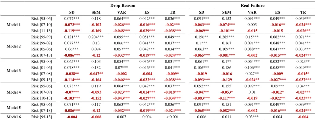
This section presents the results of the survival analysis. Table 4 shows the estimates of the model parameters as well as the hazard ratios for each of the covariates that were considered. It is important to mention that there are 5 regressions estimated in each

EMPIRICAL RESULTS

24

panel of Table 4, one for each risk measure. The failure event considered in Panel A is the Drop reason failure, while for Panel B it is the Real failure criteria.

Table 4

Results for the Survival Analysis of Hedge Funds

The table provides the estimated parameters (β) and the hazard ratios for the survival analysis of hedge funds from January 1995 to April 2013. There are 5 regressions considered in each panel of this table; one for each risk measure. The model considers two risk measure covariates for each of the two time periods (i.e., 1995-2004 and 2005-2013). Besides the two risk measures, 15 additional covariates (including the investment styles) are also considered in this model as controlling variables. The hazard ratio is the exponential of the corresponding coefficient and represents by how much does the risk of failure increases or decreases. The VaR, ES and TR are calculated with the Cornish-Fisher expansion. The values in bold correspond to the estimated coefficients for the risk measures that are negative and statistically significant. In

Panel A the failure event is defined according to the Drop reason failure while in Panel B it is defined according to the Real failure criteria. The *, ** and *** denote whether the

estimated parameters are statistically significant for a 10%, 5% and 1% levels, respectively.

Panel A - Failure Event: Drop Reason Failure

SD SEM VaR ES TR Parameters (β) Co efficie n t Ha za rd Ra ti o Co efficie n t Ha za rd Ra ti o Co efficie n t Ha za rd Ra ti o Co efficie n t Ha za rd Ra ti o Co efficie n t Ha za rd Ra ti o Risk [95-06] 0.06*** 1.07 0.1*** 1.11 0.05*** 1.05 0.04*** 1.04 0.04*** 1.04 Risk [07-13] -0.11*** 0.90 -0.16*** 0.86 -0.06*** 0.95 -0.03*** 0.97 -0.03*** 0.97 Avg Return 1Y -0.27*** 0.77 -0.27*** 0.76 -0.27*** 0.77 -0.26*** 0.77 -0.26*** 0.77 Avg AUM 1Y -0.04*** 0.97 -0.04*** 0.96 -0.04*** 0.97 -0.03*** 0.97 -0.03*** 0.97 Std AUM 1Y 0.04*** 1.04 0.04*** 1.05 0.04*** 1.05 0.04*** 1.05 0.04*** 1.04 Age 0.01 1.01 0.01* 1.01 0.01* 1.01 0.01* 1.01 0.01** 1.01 HWM -0.24*** 0.79 -0.24*** 0.79 -0.25*** 0.78 -0.24*** 0.78 -0.24*** 0.79 Personal Capital -0.04 0.96 -0.04 0.96 -0.04 0.96 -0.04 0.96 -0.04 0.96 Leveraged 0.06 1.06 0.06 1.06 0.06 1.06 0.04 1.05 0.05 1.05 Lockup 0.03 1.04 0.04 1.04 0.04 1.04 0.03 1.03 0.03 1.03 Convertible Arbitrage 0.33*** 1.40 0.34*** 1.41 0.36*** 1.44 0.38*** 1.46 0.37*** 1.45 Dedicated Short Bias 0.13 1.14 0.09 1.10 0.08 1.08 -0.06 0.94 -0.05 0.95 Equity Market Neutral 0.49*** 1.63 0.49*** 1.63 0.51*** 1.67 0.52*** 1.68 0.51*** 1.67 Event Driven 0.33*** 1.38 0.33*** 1.39 0.34*** 1.41 0.34*** 1.40 0.34*** 1.40 Fixed Income Arbitrage 0.3*** 1.34 0.29*** 1.34 0.32*** 1.38 0.32*** 1.37 0.31*** 1.37 Global Macro 0.3*** 1.35 0.29*** 1.34 0.27*** 1.31 0.25** 1.29 0.26*** 1.29 Long/Short Equity Hedge 0.22*** 1.25 0.22*** 1.25 0.22*** 1.25 0.19*** 1.21 0.19*** 1.21

25 Table 4 - Continuation

Panel B - Failure Event: Real failure criteria

SD SEM VAR ES TR Parameters (β) Co efficie n ts Ha za rd Ra ti o Co efficie n ts Ha za rd Ra ti o Co efficie n ts Ha za rd Ra ti o Co efficie n ts Ha za rd Ra ti o Co efficie n ts Ha za rd Ra ti o Risk [95-06] 0.02 1.02 0.02 1.02 0.03** 1.03 0.03*** 1.03 0.03*** 1.03 Risk [07-13] -0.18*** 0.83 -0.26*** 0.77 -0.07*** 0.93 -0.04*** 0.96 -0.04*** 0.96 Avg Return 1Y -0.5*** 0.61 -0.52*** 0.60 -0.48*** 0.62 -0.46*** 0.63 -0.46*** 0.63 Avg AUM 1Y -0.11*** 0.90 -0.11*** 0.90 -0.11*** 0.90 -0.11*** 0.90 -0.11*** 0.90 Std AUM 1Y 0.04 1.04 0.05 1.05 0.04 1.04 0.05 1.05 0.05 1.05 Age 0.02** 1.02 0.02** 1.03 0.02** 1.02 0.03** 1.03 0.03*** 1.03 HWM -0.19** 0.83 -0.2** 0.82 -0.22** 0.80 -0.22** 0.81 -0.21** 0.81 Personal Capital 0.01 1.01 0.01 1.01 < 0.01 1.01 0.02 1.02 0.02 1.02 Leveraged -0.03 0.97 -0.03 0.97 -0.05 0.95 -0.06 0.94 -0.06 0.94 Lockup 0.05 1.05 0.05 1.06 0.05 1.05 0.04 1.04 0.03 1.03 Convertible Arbitrage 0.46** 1.59 0.47** 1.61 0.54** 1.71 0.5** 1.65 0.49** 1.63 Dedicated Short Bias 0.13 1.13 0.06 1.07 0.08 1.09 -0.1 0.90 -0.09 0.92 Equity Market Neutral 0.77*** 2.15 0.77*** 2.17 0.86*** 2.36 0.84*** 2.33 0.83*** 2.30 Event Driven 0.01 1.01 0.03 1.03 0.1 1.10 0.05 1.06 0.05 1.05 Fixed Income Arbitrage 0.45** 1.56 0.46** 1.58 0.56*** 1.76 0.54*** 1.72 0.53** 1.70 Global Macro 0.52*** 1.68 0.5*** 1.65 0.48*** 1.62 0.43** 1.54 0.43** 1.54 Long/Short Equity Hedge 0.37*** 1.44 0.36*** 1.43 0.36*** 1.44 0.28** 1.33 0.29** 1.33

It is possible to infer that between 1995 and 2006 there is a positive and significant relationship between the level of risk taken by a fund and its probability of a Drop reason failure. In other words, the more risk a fund takes, the more likely it will be for a Drop reason failure to occur. This result is evident by looking at the results of the parameter Risk [95-06] in Panel A of Table 4. Furthermore, if the Real failure method is

considered, the results for the risk parameter between 1995 and 2006 are also positive. Nonetheless, whenever the Real failure method is considered, the SD and the SEM lose their explanatory power in predicting hedge fund failure. Meanwhile, the VaR, ES and TR remain statistically significant parameters for a 1% level. This result can be seen by looking at the results of the parameter Risk [95-06] in Panel B of Table 4. Converging

with these results, Liang and Park (2010) and Lee and Kim (2014) also show empirical evidence that there is a positive relation between risk and the probability of failure. Furthermore Liang and Park (2010) also show that the SD and the SEM do not have explanatory power when considering the Real failure method.

EMPIRICAL RESULTS

26

On the other hand, if we consider the time period between 2007 and 2013, the results of the risk parameter become negative and statistically significant for all of the risk measures and for both failure methods. These findings are shown by the results of the estimated parameter Risk [07-13] in Panels A and B of Table 4. Therefore, it is possible to

conclude that before 2007 higher risk levels were associated with riskier funds and from 2007 onwards this relation inverted. This is a new finding in hedge fund literature since no previous authors have ever presented empirical evidence suggesting the existence of this shift in the relation between risk and failure.

Furthermore, it is possible to quantify by how much a change in the risk level of a hedge fund affects its probability of failure through the interpretation of the hazard ratios depicted in Table 4.10 For example, during the period between 1995 and 2006, if the ES of a hedge fund increased by one unit, it meant the risk of occurrence of a Real failure would grow by 3%. This finding is evident by looking at the results of the hazard ratio for the parameter Risk [95-06] in Panel B of Table 4. On the other hand, having a

hazard ratio below 1 implies the existence of an inverse relation between the covariate and the risk of failure. Hence, for the period between 2007 and 2013, an increase of one unit in the ES will reduce the probability of a Real failure by 4%. This finding is evident by looking at the results of the hazard ratio for the parameter Risk [07-13] in Panel B of

Table 4.

Ben-David, Franzoni and Moussawi (2012) find that, during the Global Financial Crisis, more than low-volatility stocks were sold by hedge funds due to the fact that high-volatility positions required a greater amount of margins. Therefore, it is possible to infer that funds that were faced with financial constraints attempted to decrease their risk profile. Bearing this in mind it is possible to hypothesize that, even though these “stressed” funds were able to adopt a lower risk profile, ultimately they were incapable of overcoming their financial limitations, thus failing. On the other hand, funds that did not experience financial constraints during the Global Financial Crisis were able to maintain their previous risk levels. This way, the response of hedge funds to the Global Financial Crisis could have caused a shift in the dynamics between risk and failure. It is important to mention that this is a hypothetical reason for the occurrence of this shift

10 _{If the value of a certain covariate increases by one unit, and the hazard ratio of that covariate is HR, the}

27 and that further research about the portfolio allocation of hedge funds during this period could potentially shed a light on this matter.

Regarding the remaining covariates, results show the last year performance and size of the fund decrease the risk of failure of hedge funds. In other words, funds that perform better and have more AuM are less likely to fail relatively to funds that have a lower performance and are smaller in size. This conclusion can be taken from the estimated parameters for the Avg Return 1Y and Avg AUM 1Y which are always negative and statistically significant for a 1% level for both failure events considered in the analysis. In line with these results are the findings of Liang and Park (2010), Haghani (2014) and Lee and Kim (2014) who also perform a survival analysis and show negative coefficients for the covariates of the RoR and the AuM of hedge funds.

Furthermore, it is also possible to see that having a HWM also reduces the risk of failure. Liang and Park (2010) show similar results and argue that having a HWM provision serves as a manager quality signal since only good fund managers can afford to impose this condition. Additionally, Liang (1999) argues that funds with HWM significantly outperform those without. Moreover, the age covariate is associated with a positive coefficient which diverges from the findings of Liang and Park (2010) by suggesting older funds are more likely to fail.

All of the estimated parameters for the investment style covariates are statistically significant with the exception of the Dedicated Short Bias investment style for both panels of Table 4 and the Event Driven investment style for Panel B. These findings suggest that generally, the investment style adopted by a fund influences its risk of failure which is related with the fact that the overall performance of hedge funds varies according to its investment style. This idea can be supported by the findings of Brown and Goetzmann (2003) who argue that differences in investment style contribute for about 20 per cent of the cross-sectional variability in hedge funds performance. Moreover, Liang and Park (2010) and Haghani (2014) also find that certain investment styles have explanatory power in predicting the hedge fund failure.

On the other hand, Table 4 suggests that the Std AUM 1 Y, Personal Capital, Leveraged and Lockup parameters are not statistically significant in predicting hedge fund failure. The results for these three parameters go in line with the article of Liang and Park (2010). Furthermore, Haghani (2014) also finds that having leverage is not a statistically