i
Next Best Action – a Data-Driven Marketing
Approach
João Luís Trindade Milheiro
Work Project report presented as partial requirement for
obtaining the Master’s degree in Advanced Analytics
ii
NOVA Information Management School
Instituto Superior de Estatística e Gestão de Informação
Universidade Nova de LisboaNEXT BEST ACTION – A DATA-DRIVEN MARKETING APPROACH
by
João Luís Trindade Milheiro
Work Project report presented as partial requirement for obtaining the Master’s degree in Advanced Analytics
Advisor: Mauro Castelli
iii
DEDICATION
iv
ACKNOWLEDGEMENTS
I thank Magdalena Neate from the bottom of my heart for giving me the space to be creative and challenged in this big project.
I also thank my parents and my godmother for always believing in me. Finally, I thank professor Mauro Casteli for accepting to be my advisor.
v
ABSTRACT
The Next Best Action (NBA) is a framework that is built in order to assign to each client three (or more) actions that are considered to be the best actions to perform with the client. These actions can range from product offering to pro-active retention actions and upselling recommendations. It can be a useful tool to generate leads for ongoing campaigns but also an excellent tool for analysis and a driver for the creation of new campaigns, being a key element in Customer Relationship Management (CRM) as a Data-Driven Marketing approach.
Initially planned as a joint collaboration between a Bank and an Insurance Company to improve the Bancassurance business model, three versions of the NBA were built with the first two being tested on a campaign setting showing promising results. The last version, NBA 3.0, later became a sole project of the Insurance Company due to GPDR compliance policies and due to time constraints could not be evaluated.
KEYWORDS
Next Best Action; Customer Relationship Management; Data-Driven Marketing; Bancassurance; GDPR
vi
INDEX
1.
Introduction ... 1
2.
Literature review ... 4
2.1.
Customer Relationship Management (CRM) ... 4
2.2.
Data-Driven Marketing ... 5
2.3.
Next Best Offer and Next Best Action ... 6
2.4.
General Data Protection Regulation ... 6
2.5.
Data Science and SAS® ... 7
2.6.
Machine Learning Algorithms ... 10
3.
Next Best Action ... 15
3.1.
Project Scope ... 15
3.2.
Project Roadmap ... 16
3.3.
Phase One – Before GDPR ... 18
3.3.1.
Defining the Actions ... 18
3.3.2.
NBA 1.0 ... 16
3.3.3.
NBA 2.0 ... 28
3.4.
Phase Two – After GDPR ... 41
3.4.1.
NBA 3.0 ... 42
3.5.
Deployment of the NBA Framework ... 45
4.
Limitations and recommendations for future works ... 47
5.
Bibliography ... 49
vii
LIST OF FIGURES
Figure 1.1 - Moving from Product Perspective to a Costumer Perspective (Alexander Hesse
2009) ... 2
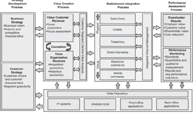
Figure 2.1 - Conceptual Framework of CRM Strategy (Payne and Frow 2005) ... 4
Figure 2.2 - Diagram of Data-Driven Decision Making (Provost and Fawcett 2013) ... 5
Figure
2.3
–
Integration
of
GDPR
in
Data-Driven
Marketing
Strategies
(
https://blog.hubspot.com/customers/gdpr-data-features-hubspot-compliance
) ... 7
Figure 2.4 - Various areas where Data Science is a key element (
http://www.sas.com
) ... 8
Figure 2.5 - Example of a Decision Tree ... 10
Figure 2.6 - Example of a Logistic Regression ... 11
Figure 2.7 - Simplified Neural Network ... 12
Figure 2.8 - Neural Network with two hidden layers (
https://towardsdatascience.com/applied-deep-learning-part-1-artificial-neural-networks-d7834f67a4f6
) ... 13
Figure 2.9 - Example of a ROC curve ... 14
Figure 3.1 - Exchange of Information between the Bank and the Insurance Company before
and after the implementation of GDPR procedures ... 15
Figure 3.2 - Project Roadmap - Phase One ... 16
Figure 3.3 - Project Roadmap - Phase Two ... 17
Figure 3.4 - Map of NBAs used in NBA 2.0 ... 19
Figure 3.5 - Ownership Model Universe ... 18
Figure 3.6 - Cumulative Lift of Model Ensemble, Logistic Regression and Neural Networks
models ... 20
Figure 3.7 - Backtesting results of the Health Model ... 21
Figure 3.8 - Temporal window for the Personal Accidents Model ... 22
Figure 3.9 - Relative Importance of the Groups of Selected Variables of the Personal Accidents
Model ... 23
Figure 3.10 - Undersampling scheme ... 23
Figure 3.11 - ROC Curve of the Neural Network ... 24
Figure 3.12 - Backtesting of the Neural Network in more recent data ... 25
Figure 3.13 – NBA 1.0 Formula ... 26
Figure 3.14 - Confidence Formula ... 27
viii
Figure 3.16 - Assignment of Testing Groups ... 33
Figure 3.17 - Absolute Number of Sales of the Auto Inbound Campaign ... 34
Figure 3.18 - Absolute Number of Sales of the Auto Inbound Campaign ... 34
Figure 3.19 - Contact Rate of the Auto Inbound Campaign ... 35
Figure 3.20 - Contact Rate of the Health Inbound Campaign ... 36
Figure 3.21 - Intention Rate of the Auto Inbound Campaign ... 37
Figure 3.22 - Intention Rate of the Health Inbound Campaign ... 37
Figure 3.23 - Sales Rate of the Auto Inbound Campaign ... 38
Figure 3.24 - Sales Rate of the Health Inbound Campaign ... 39
Figure 3.25 - Sales Rate of the Auto Inbound Campaign (by type of NBA) ... 39
Figure 3.26 - Sales Rate of the Health Inbound Campaign (by type of NBA) ... 40
Figure 3.27 - NBA 3.0 Calculation Formula ... 44
Figure 3.28 - Possible Deployment of the NBA Framework ... 46
Figure 6.1 – Digital Channels provided by Financial Institutions – Source: Banco de Portugal
... 52
ix
LIST OF TABLES
Table 2.1 - Key Terms in Data Science (Cao 2017) ... 8
Table 2.2 - Logistic Regression sample example ... 11
Table 3.1 - Models built between the Bank and the Insurance Company for Insurance Products
... 16
Table 3.2 - Human Health Business Activity Code (Institituto Nacional de Estatística 2007) .. 18
Table 3.3 - Health Model Universe ... 19
Table 3.4 - Backtesting Groups ... 21
Table 3.5 - Personal Accidents Model Universe ... 22
Table 3.6 - Groups of Selected Variables ... 23
Table 3.7 - Fit Statistics of the Personal Accidents Models ... 24
Table 3.8 - Example of NBA calculation ... 26
Table 3.9 - Confidence Levels ... 27
Table 3.10 - NBA calculation without simulations information (NBA 1.0) ... 31
Table 3.11 - NBA calculation including simulations information ... 31
x
LIST OF ABBREVIATIONS AND ACRONYMS
AI Artificial Intelligence ANN Artificial Neural Networks
CRM Customer Relationship Management DPD Data Protection Directive
EU European Union FN False Negative FP False Positive
GDPR General Data Protection Regulation IT Information Technology
LoB Line of Business ML Machine Learning MSE Mean Squared Error NBA Next Best Action NBO Next Best Offer
ROC Receiver Operating Curve TN True Negative
1
1. INTRODUCTION
With vast amounts of data now available, companies in almost every industry, like banking and insurance, are focused on exploiting data for competitive advantage against other companies. We live in the era of Big Data and the volume and variety of data have far outstripped the capacity of manual analysis, and in some cases have exceeded the capacity of conventional databases, requiring each time more processing power. At the same time, computers have become far more powerful, networking is ubiquitous, and algorithms have been developed that can connect datasets to enable broader and deeper analyses (Provost and Fawcett 2013), leading companies to turn their heads to Data Science and its unlimited potentialities.
According to the definition of the Center for Insurance & Financial planning, “Bancassurance assume a wide range of detailed arrangements between banks and insurance companies, but in all cases it includes the provision of insurance and banking products or services” (Clipici 2012). Mutual cooperation and strategic alliance are omnipresent in present global economy and Bancassurance has proven to be quite successful in Europe (Wu, Lin, and Lin 2009), being heavily present in the Portuguese market, with a market share reaching 87% in Portugal in 2009, arising as the most popular distribution channel for life insurance policies in Portugal. (Clipici 2012).
Living in the digital era, Bancassurance executives are still struggling to devise the perfect cross-channel experiences for their customers—experiences that take advantage of digitization to provide customers with targeted, just-in-time product or service information in an effective and seamless way (Bommel, Edelman, and Ungerman 2014) although almost 90% of the Financial Institutions provide digital channels to their customers (Figure 6.1 – Digital Channels provided by Financial Institutions – Source: Banco de Portugal).
Digital channels allow companies to collect a large amount of data on customer interactions with the company, its agents and products, as well as interactions between customers and other prospects or customers. However, the customer journey cannot be considered solely through the prism of digital marketing. Contact points can involve any agent in the company, computer-tracked interactions with objects, interactions with points of sale and systems, and digital and direct contacts through the media. As all departments of the company are involved, the data are a common ground for collaboration (Micheaux and Bosio 2019).
With all this data gathered, a change in the marketing paradigm is needed and the focus, which was the product, now shifts to the client, becoming a client-centered vision (Alexander Hesse 2009). Using customer data to help the customer while making a profit represents a service for both the customer and the company and society. The use of data to produce relevant and timely marketing proposals is a service to the customer. The data serve the company through the revenues they generate and serve society through the employment they create (Micheaux and Bosio 2019). This leads to the definition of Next Best Offer (NBO) and Next Best Action (NBA) - Figure 1.1.
Despite the name, an NBO/NBA may in fact be an initial engagement. And whether the customer relationship is new or ongoing, the NBO/NBA is intended to be a “best offer/action” (Davenport, Mule, and Lucker 2011).
2 Figure 1.1 - Moving from Product Perspective to a Costumer Perspective (Alexander Hesse 2009)
Being Bancassurance a synergism between different companies, since May 25th 2018, the General Data Protection Regulation (GDPR) became in full effect, demanding companies to review their data exchange policy and adapt it to the new regulation. The GDPR expands the scope of data protection so that anyone or any organization that collects and processes information related to EU citizens must comply with it, no matter where they are based or where the data is stored (Tankard 2016).
Considering the importance of a customer-centric marketing approach, and working as a Business Analytics consultant for an IT company, I was approached by a Financial Institution (mentioned as the Bank) and their corresponding Insurance Company Bancassurance partner to help them design and create a framework to assign to each client three NBAs (regarding insurance products) to help them prioritize lead generation for all their campaigns, focusing their marketing strategy on the client, utilizing different inputs such as predictive models scores, previous campaign contacts, policy simulations and business rules imposed by both companies, focusing on clients from both companies (Bancassurance clients) to maximize the insights gathered from both sides of the company; and clients without any kind of insurance (Bank-only clients) as a way of selecting the best new clients.
The main idea of the NBA framework was to assign to each client 3 (or more) actions that are considered to be the best actions for the client, ranging from product offering, to retention and upselling pro-active actions with the prospection of adding new and diverse actions in future improvement versions of the framework.
The NBA project was crucial to help understanding how a data-driven marketing strategy can be used to improve business, especially in the Customer Relationship Management of the Bancassurance business model.
3 1. Analysis of the predictive models already used;
2. Building of new predictive models for Lines of Business (LoB) without an assigned model; 3. Definition of the actions to be considered as NBAs;
4. Calculation of the NBA and its corresponding confidence levels;
5. Testing NBA in terms of inbound campaigns and dashboarding the results; 6. Adjusting NBA calculation with insights derived from weekly campaign results; 7. Defining integral deployment of the NBA and future improvements.
Analysis of the existing models and building of new ones was possible using SAS® data mining software, mainly SAS® Enterprise Miner, by using some Machine Learning algorithms.
Initially planned to be a one phase work project, the NBA design was divided in two phases spanned across a time period of 10 months (December 2018 – September 2019):
Phase One: creation of a client-centralized table used for the calculation of the NBA and its corresponding confidence and a weekly dashboard showing the results of the NBA in terms of inbound campaigns for all clients (Bancassurance and bank-only clients), December 2018 – June 2019;
Phase Two: redesign of the NBA framework applied to Bancassurance clients, July 2019 – September 2019 (this reformulation was a side-effect of the impact of GDPR policies implemented by the bank).
4
2. LITERATURE REVIEW
2.1.
C
USTOMER
R
ELATIONSHIP
M
ANAGEMENT
(CRM)
Over the last years, there has been an explosion of interest in CRM from Bancassurance and other commercial fields and, despite an increasing amount of published practical material, there remains a lack of agreement about what CRM is, how CRM strategy should be developed (Payne and Frow 2005) and which steps are required to transition from a mass-marketing culture to a business environment for one-to-one marketing (Kelly 2000).
The term “customer relationship management” emerged in the information technology (IT) community in the mid-1990s to describe technology based customers solutions (Payne and Frow 2005) but one of the most solid definitions is given by Ronald Swift in his book “Accelerating Customer Relationships— Using CRM and Relationship Technologies”:
CRM is a strategic approach that is concerned with creating improved shareholder value through the development of appropriate relationships with key customers and customer segments. CRM unites the potential of relationship marketing strategies and IT to create profitable, long-term relationships with customers and other key stakeholders. CRM provides enhanced opportunities to use data and information to both understand customers and cocreate value with them. This requires a cross-functional integration of processes, people, operations, and marketing capabilities that is enabled through information, technology, and applications.
5 In short, CRM is a business strategy dedicated to creating and maintaining a long- term and profitable relationships with clients. The basic prerequisite for CRM implementation is to collect information about customers/users, analysis of these data, exchange and tracking (Greenberg 2010).
One of the main objectives of the NBA is to optimize CRM and maximize client satisfaction, alongside increasing the revenue for both the Bank and the Insurance Company, for satisfied clients reward companies with loyalty and commitment (Yu and Dean 2001).
2.2.
D
ATA
-D
RIVEN
M
ARKETING
Marketing strategy means setting out business direction and the allocation of resources that create customer value, it is about choosing value, providing value and communicating value to customers (Hanssens 2002).
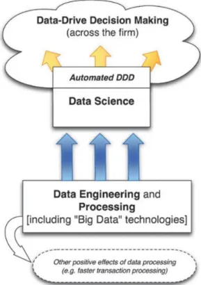
Data-driven decision making refers to the practice of basing decisions on the analysis of data rather than purely on intuition (Provost and Fawcett 2013) and extracting useful knowledge from data to solve business problems is the foundation of the NBA framework (Figure 2.2).
Speed, price and availability of numerous software solutions highlight the advantages of this Marketing philosophy but its lack of methodologies, difficulties in interpretation and verification of achieved results surface as the prime disadvantages of Data-Driven Marketing (Shankar 2016).
Data science supports data-driven decision making—and sometimes allows making decisions automatically at massive scale—and depends upon technologies for ‘‘big data’’ storage and engineering. However, the principles of data science are its own and should be considered and dis- cussed explicitly (Provost and Fawcett 2013) bearing in thought business rules should also be used in certain cases and/or problems, with these business rules being of the inputs thought for the NBA calculation.
A ‘customer focused’ marketing strategy in response to the changes in the market place is the most important element in deriving a successful next product to offer plan (Lau et al. 2003).
Figure 2.2 - Diagram of Data-Driven Decision Making (Provost and Fawcett 2013)
6
2.3.
N
EXT
B
EST
O
FFER AND
N
EXT
B
EST
A
CTION
Typical questions raised by Bancassurance marketers to better understand customers are: Which product does this customer need? Can he/she afford the products? Has he/she already bought the product from competitors? How much discount should the bank offer to him/her to close the sale? What is the most effective communication message to stimulate his/her interest in the product? (Lau et al. 2003), questions which raise the importance of the definition of NBA.
NBO/NBA is increasingly used to refer to a proposal customized based on the consumer’s attributes and behaviors, the purchase context, product or service characteristics and the organization’s strategic goals. They are most often designed to inspire a purchase, drive loyalty, or both, consisting of products, services, information and relationships (Davenport, Mule, and Lucker 2011).
A ‘customer focused’ marketing strategy in response to the changes in the market place is the most important element in deriving a successful next product to offer plan (Fletcher 2002).
2.4.
G
ENERAL
D
ATA
P
ROTECTION
R
EGULATION
On 27th April 2016, after four years of drafting, lobbying and negotiations among the EU Member States and many affected organizations, the EU General Data Protection Regulation (GDPR) has been agreed and finalized, whereas on 4th May 2016 its final text was published in the Official Journal of the European Union (Regulation 2016/679).
Previous data protection legislation had become fragmented across the EU as different countries added to the basic principles enshrined in the original directive (DPD) of 1995 (Tankard 2016) leaving behind a need to legislate the usage of personal data.
Many of the core definitions from the DPD remain largely unchanged with GDPR complying with six processing principles, stating that personal data shall be:
1. Processed lawfully, fairly and transparently; 2. Collected for specific legitimate purposes only; 3. Adequate, relevant and limited to what is necessary; 4. Accurate and kept up to date;
5. Stored only as long as is necessary;
6. Protected with appropriate security measures, ensuring its integrity and confidentiality. This new law covers the personal data of all EU residents, regardless of the location of the processing. Personal data is information that, directly or indirectly, can identify an individual, and specifically includes online identifiers such as IP addresses, cookies and digital fingerprinting, and location data that could identify individuals (Goddard 2017).
With GDPR all EU citizens are entitled to demand a company to delete all the information they have about them (“right to be forgotten”), ask for a back-up of all the information stored in the company including third-party companies which the information was given to and all citizens and have to be notified for any breach of the GDPR in less than 72 hours. Infringement of the EU GDPR can result in
7 administrative fines of up to 4% of annual global turnover or €20 million – whichever is greater (Regulation 2016/679), imposing greater requirements for data privacy, for example, like the right to data portability (the right to order a company to transfer the personal data to other companies) and the “right to be forgotten” (Safari 2017).
The GDPR extends the provision on automated individual decision-making, to include profiling cases as a prime example of enabling individuals to control their personal data in the context of automated decision-making (Article 22) and hence acts as crucial function for mitigating the risks of big data and automated decision making for individual rights and freedoms (Politou, Alepis, and Patsakis 2018). This proved to be one of the biggest challenges faced in Bancassurance: the client has to give explicit consent for the exchange of data between companies and for the treatment of the same data. Consent aims at providing legitimate grounds to data controllers for collecting, processing or even disseminating personal data for secondary use (Edwards 2017).
Figure 2.3 – Integration of GDPR in Data-Driven Marketing Strategies (https://blog.hubspot.com/customers/gdpr-data-features-hubspot-compliance)
New innovative concepts like the right to data portability, standardized privacy icons and data protection by design and default are opening wide opportunities to foster innovation and competition in the direction of data protection and consumer friendly products and services (Albrecht 2017). Being Bancassurance a symbiosis between different companies, all the procedures must comply with GDPR, including the NBA framework.
2.5.
D
ATA
S
CIENCE AND
SAS®
In 1996, for the first time, the term Data Science was included in the title of a statistical conference (International Federation of Classification Societies (IFCS) “Data Science, classification, and related methods”) emphasizing the importance of Statistics in Classification Methods (such as Clustering) with some use cases (Hayashi et al. 1996).
8 Even though Statistics is one of the most important disciplines to provide tools and methods to find structure in and to give deeper insight into data (Weihs and Ickstadt 2018), the term Data Science has become an umbrella term describing a discipline typically involving a mixture of statistics and large-scale computing (Hardin et al. 2015) with Australian Longbing Cao formulating Data Science as the harmonious combination of Statistics, Computing, Communication, Sociology and Management on the basis of data, the environment and the so called data-to-knowledge-to-wisdom thinking (Cao 2017):
Data Science = (Statistics + Computing + Communication + Sociology + Management) | (Data + Environment + Thinking)
Figure 2.4 - Various areas where Data Science is a key element (http://www.sas.com)
Cao highlighted key terms used in Data Science, summarizing all the present ideas we have about Data Science and Analytics - Table 2.1 - Key Terms in Data Science (Cao 2017).
Table 2.1 - Key Terms in Data Science (Cao 2017)
KEY TERMS DEFINITION
ADVANCED ANALYTICS
Refers to theories, technologies, tools, and processes that enable an in-depth understanding and discovery of actionable insights in big data, which cannot be achieved by traditional data analysis and processing theories, technologies, tools, and processes.
BIG DATA Refers to data that are too large and/or complex to be effectively and/or
efficiently handled by traditional data-related theories, technologies, and tools.
DATA ANALYSIS
Refers to the processing of data by traditional (e.g., classic statistical,
mathematical, or logical) theories, technologies, and tools for obtaining useful information and for practical purposes.
DATA ANALYTICS
Refers to the theories, technologies, tools, and processes that enable an in-depth understanding and discovery of actionable insight into data. Data analytics consists of descriptive analytics, predictive analytics, and prescriptive analytics.
DATA SCIENTIST Refers to those people whose roles very much center on data.
DESCRIPTIVE ANALYTICS Refers to the type of data analytics that typically uses statistics to describe the
9 PREDICTIVE ANALYTICS Refers to the type of data analytics that makes predictions about unknown future
events and discloses the reasons behind them, typically by advanced analytics.
PRESCRIPTIVE ANALYTICS Refers to the type of data analytics that optimizes indications and recommends
actions for smart decision-making.
EXPLICIT ANALYTICS Focuses on descriptive analytics typically by reporting, descriptive analysis,
alerting, and forecasting.
IMPLICIT ANALYTICS Focuses on deep analytics, typically by predictive modeling, optimization,
prescriptive analytics, and actionable knowledge delivery.
DEEP ANALYTICS
Refers to data analytics that can acquire an in-depth understanding of why and how things have happened, are happening, or will happen, which cannot be addressed by descriptive analytics.
Deriving from Data Science, the term Data Scientist was coined in 2008, by D.J. Patil and Jeff Hammerbacher, the respective leads of data and analytics efforts at LinkedIn and Facebook, and has been used to address data professionals who are skilled in organizing and analyzing massive amounts of data, being referenced as the “the sexiest job of the 21st century” (Davenport and Patil 2012). Through a quick search in LinkedIn for jobs with the title “Data Scientist”, one job advertisement came to prominence for BNP Paribas (https://www.linkedin.com/jobs/view/1477159004), where they were asking for someone with 2 to 5 years of work experience, having:
Knowledge of databases and associated tools (SQL and NoSQL) Knowledge of ETL methods (data imputation, data cleaning)
Knowledge of at least one Machine Learning development stack (e.g. Numpy, scikit-learn, keras, …)
Strong programming skills (e.g. Python, R, Java, Go, Javascript) and algorithmic knowledge Exposure to Hadoop ecosystems
Knowledge of NLP techniques
Knowledge of deep learning architectures and frameworks (e.g. TensorFlow, Keras, …) Knowledge of advanced reporting tools (Tableau, Qlikview)
It appears Data Scientists are expected to have an extended knowledge on a variety of subjects, from databases, ETL methods, Machine Learning and Programming Languages, Deep Learning and Natural Language Processing techniques, hence the reason why Data Scientists are sometimes called Unicorns (Baškarada and Koronios 2017) – finding someone with every single one of these requirements and knowledges is virtually impossible.
Despite the fact that R and Python are well known for their flexibility and being open source programming languages (Ozgur et al. 2017), according to Data Driven Investor, SAS® is one of the biggest Data Science programming languages and, although lacking the ease to incorporate open source features like R and Python, SAS® has an excellent support system, being one of the biggest advantages regarding open source programming languages (Bachheriya 2019). As of 2019 100% of Fortune 500 companies in the areas of Commercial Banking, Health Insurance, Pharmaceutical,
10 Aerospace Manufacturing, E-Commerce, Computer Services and Retail Banking rely on SAS®, being a leader in Analytics (SAS 2019).
SAS® has been present in Portugal for the last 25 years with great strength in banking and insurance companies and was the selected tool for modelling and calculation of the entire NBA framework.
2.6.
M
ACHINE
L
EARNING
A
LGORITHMS
In 1959, Arthur Samuel defined Machine Learning (ML) as the subfield of Artificial Intelligence (AI) that “gives computers the ability to learn without being explicitly programmed” (Samuel 1959) and over the last quarter of a century, ML has become one of the most important parts of the IT revolution impacting our lives.
Although ML dates from the early days of AI in the late 1950s, it underwent a first resurgence when the concept of data mining began to takeoff approximately 20 years ago. Data mining algorithms look for patterns in information. ML does the same thing but goes one step further: the program changes its behavior based on what it learns (Lee et al. 2017).
Numerous ML algorithms have been developed and extensively documented, but this project focused on some of the algorithms of supervised learning, learning a function that maps an input to an output based on example input-output pairs (Russel and Norvig 2010), present in SAS® Enterprise Miner, the SAS® software which was used for this project:
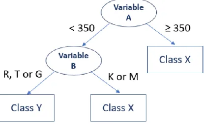
Decision Tree
A decision tree is a classifier which conducts recursive partition over the instance space. A typical decision tree is composed of internal nodes, edges and leaf nodes. Each internal node is called decision node representing a test on an attribute or a subset of attributes, and each edge is labeled with a specific value or range of value of the input attributes. In this way, internal nodes associated with their edges split the instance space into two or more partitions. Each leaf node is a terminal node of the tree with a class label (Wei and Wei 2014).
11 Figure 2.5 exemplifies a basic decision tree, where circle means decision node and square means leaf node. In this example, there are two splitting attributes (Variable A and Variable B), along with two class labels (Class X and Class Y). Each path from the root node to leaf node forms a classification rule.
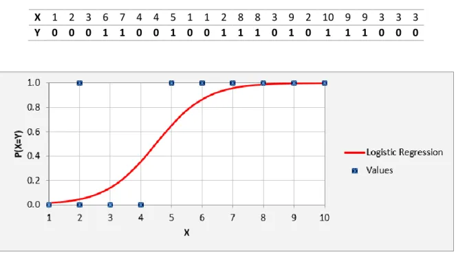
Logistic Regression
A logistic regression is used to model the probability of a certain class or event existing such buying/not buying. It is a statistical model that in its basic form uses a logistic function to model a binary dependent variable. This model estimates the parameters of a logistic model (a form of binary regression) (Cox 1958).
Assuming 𝑋1, … , 𝑋𝑛are independent variables and 𝑌 is the independent variable assuming only two
categorical values (0 or 1):
𝑃(𝑋 = 𝑌) = 1
1 + 𝑒−(𝛽
0+ 𝛽1𝑋1+ ⋯ + 𝛽𝑛𝑋𝑛)
Where 𝛽0, 𝛽1, … , 𝛽𝑛are the estimates of the parameters of the logistic regression. With the estimation
of the parameters, a probability for the event in study can be calculated for all individuals.
Imagining a sample (Table 2.2) is obtained where X is the independent variable and Y is the event “Red/Blue” coded as 1 (“Red”) and 0 (“Blue”). A logistic regression can estimate the parameters and a graph can be traced (Figure 2.6).
Table 2.2 - Logistic Regression sample example
X 1 2 3 6 7 4 4 5 1 1 2 8 8 3 9 2 10 9 9 3 3 3 Y 0 0 0 1 1 0 0 1 0 0 1 1 1 0 1 0 1 1 1 0 0 0
12 Neural Network
Artificial Neural Networks (ANN) are a set of algorithms, modeled loosely after the human brain, that are designed to recognize patterns and can be defined as “an interconnected assembly of simple processing elements, units or nodes, whose functionality is loosely based on the animal neuron. The processing ability of the network is stored in the interunit connection strengths, or weights, obtained by a process of adaptation to, or learning from, a set of training patterns” (Gurney 1997).
ANNs can be used to perform probabilistic functions in either a hardware or software analogue. These systems are designed to operate in the same manner in which the neurons and synapses of the brain are theorized to operate. The architecture of neural connections can be described as a combinational feedforward network. Artificial neurons operate by summing inputs (x1, x2, x3) individually scaled by weight factors (w1,w2,w3) and processing that sum with a nonlinear activation function, most often approximating the logistic-function: 1/(1+exp(−x)) which returns a real value in the range (0,1) (Pagel and Kirshtein 2017).
Figure 2.7 - Simplified Neural Network ANNs are constructed from 3 type of layers (Figure 2.7):
Input layer — initial data for the neural network.
Hidden layers — intermediate layer between input and output layer and place where all the computation is done.
Output layer — produce the result for given inputs.
13 Figure 2.8 - Neural Network with two hidden layers (
https://towardsdatascience.com/applied-deep-learning-part-1-artificial-neural-networks-d7834f67a4f6) Model Ensemble
Ensemble modeling is a process where multiple diverse models are created to predict an outcome, either by using many different modeling algorithms or using different training data sets. The ensemble model then aggregates the prediction of each base model and results in once final prediction for the unseen data. The motivation for using ensemble models is to reduce the generalization error of the prediction. As long as the base models are diverse and independent, the prediction error of the model decreases when the ensemble approach is used. The approach seeks the wisdom of crowds in making a prediction (Kotu and Deshpande 2015).
For choosing the “best” model (the No Free Lunch Theorem states there is no one model that works best for every problem) there are a range of statistics used to assess the perform of the predictive model, like:
Mean Squared Error (MSE)
The MSE assesses the quality of a ML algorithm by measuring the average squared difference between the estimated values (𝑌̂𝑖) and the actual value (𝑌𝑖) (Lehmann and Casella 1998).
𝑀𝑆𝐸 = 1
𝑛∑(𝑌𝑖− 𝑌̂𝑖)
2 𝑛
𝑖=1
The closest the value is to 0, the better the model predictor. Lift
The lift is probably the most commonly used metric to measure the performance of targeting models in marketing applications. A targeting model is doing a good job if the response within the target is much better than the average for the population as a whole (Coppock 2002).
Lift is the ratio of the target response divided by average response: Lift = Target %
14 For example, suppose a population has an average response rate of 5%, but a certain model has identified a segment with a response rate of 35%. Then that segment would have a lift of 7 (35%/5%).
Area under the ROC Curve
When dealing with a two class classification problems we can always label one class as a positive and the other one as a negative class. A classifier assigns a class to each of them, but some of the assignments are wrong. To assess the classification results the number of true positive (TP), true negative (TN), false positive (FP) (actually negative, but classified as positive) and false negative (FN) (actually positive, but classified as negative) where:
TP + FN = Positives TN + FP = Negatives FPRate = FP N TPRate= Recall = TP P Precision = TP TP+FP Accuracy = TP+TN P+N The ROC (Receiver Operating Characteristic) curve is defined by:
𝑥 = FPRate (𝑡) and 𝑦 = TPRate(𝑡),
where 𝑡 is the value of probability taken into consideration being selected all the individuals whose score is less than 𝑡 (Vuk and Curk 2006).
The area under the ROC curve (AUROC) can be used as a measure of quality of a predictive model. A random classifier (e.g. classifying by tossing up a coin) has an area under curve of 0.5, while a perfect classifier has 1. Classifiers used in practice should therefore be somewhere in between, preferably close to 1 (Vuk and Curk 2006).
Models can also be tested by using backtesting by applying the chosen model in historical data and compare the model and the actual results.
15
3. NEXT BEST ACTION
3.1.
P
ROJECT
S
COPE
Nowadays, companies are expected to hire teams that understand how to use databases and other data warehouses, scrape data from Internet sources, program solutions to complex problems in multiple languages (Hardin et al. 2015). Both the Bank and the Insurance Company possess in their Marketing Department two teams specialized in Data Mining and Modelling, teams to which I belonged during the scope of the entire NBA project.
The main focus and goal of this work project was to design a NBA framework aiming at insurance products. This framework was built in order to assign to each client three (or more) actions that were considered to be the best actions to perform with the client, whenever the calculation was possible. This NBA should take into consideration not only scores from predictive models but also other events and triggers such as simulations, contacts and some key transactions.
These actions can range from product offering to pro-active retention actions and upselling recommendations. It can be a useful tool to generate leads for ongoing campaigns but also an excellent tool for analysis, a driver for the creation of new campaigns and potentially identify new clients (not all clients from the Bank are clients of the Insurance Company).
This project was intended to be a one phase project, being supported by both the Bank and the Insurance Company as a complement for the Bank since a Next Best Offer (for all the Bank LoBs) recommendation system was being constructed at the same time, with NBA being focused solely on insurance products. Both entities were exchanging client information (being all this data codified) in a synergism extremely useful for the designing of the NBA. Predictive models were built on both sides and the scores were shared making sure all Bank clients, insured or not by the Insurance Company, were being scored for at least the propensity to buy a specific insurance LoB.
After the framework was completed, this exchange of data between both companies was drastically transformed due to the implementation of GDPR compliance procedures and the only information exchanged between the two companies was the list of eligible clients for insurance campaigns and the contacts and results of the corresponding campaigns. Because of all these restrictions, the NBA framework had to be discontinued and redesigned in the Insurance
Figure 3.1 - Exchange of Information between the Bank and the Insurance Company before
and after the implementation of GDPR procedures
16 Company side, focusing only on the Insurance Company clients, losing the uninsured Bank clients which were being treated as prospect clients.
3.2.
P
ROJECT
R
OADMAP
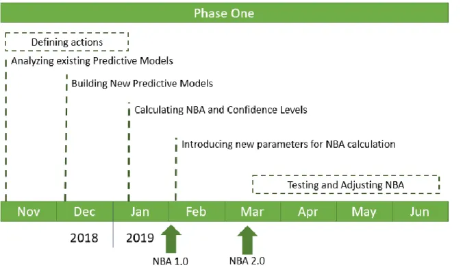
The original roadmap of the project (known as Phase One) was intended to be completed in the first semester of 2019 before knowing GDPR procedures would affect the final product.
The first step was to define the actions that would be used for the first version of the NBA (nicknamed NBA 1.0) – which would be based primarily in predictive models – and analyze existing predictive models used for defining campaign leads for the products taken into consideration for the actions. If a product didn’t have a predictive model associated to its ongoing campaigns, it should be built. The last step of the first version was to define the calculation formula of the NBAs and theirs corresponding confidence levels.
The second step was the introduction of new parameters in the NBA (such as product simulations) and testing and adjusting the NBA by using the Insurance Inbound Campaigns of two LoBs and analyzing their weekly results. This was an iterative process and was extremely useful to understand how to incorporate feedback from campaigns in the NBA calculation. It was also crucial in understanding one of the problems we were having in the first results of the NBA testing, which were not great and were putting the effort and time spent in this project in question.
Figure 3.2 - Project Roadmap - Phase One
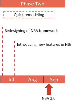
When the Testing and Adjusting phase were in full speed, there was a defining turning point in the project: the Bank and the Insurance Company, to comply with the norms of GDPR, ceased to exchange information between both companies except for the list of clients to be used in the insurance companies.
17 The exchange of all variables, even though they were codified, and models scores ceased and the testing and adjusting of NBA 2.0 had to be stopped and scrapped.
After this fateful event, the NBA project stopped being a joint effort between the Bank and the Insurance Company and the latter assumed total control of the project. By assuming the project, NBA turned its focus only on Insurance Clients, reducing drastically the client pool which was serving as the base of NBA 1.0 and 2.0 (all Bank clients regardless owning Insurance products or not).
All the predictive models which were using Bank variables as inputs had to be rebuilt in a short period of time, the NBA framework had to be rethought and redesigned (now known as NBA 3.0) and some features were added while other Bank exclusive features could not be incorporated.
After NBA 3.0 was concluded, a possible deployment solution was presented and started its testing. Unfortunately, the time allocated to me for this project ran out I could not analyze the results of the “new” NBA framework.
18
3.3.
P
HASE
O
NE
–
B
EFORE
GDPR
Initially thought as the only phase of the NBA project, Phase One was divided in two major moments: NBA 1.0 and NBA 2.0.
The NBA framework was designed as a table with useful information about the customer, containing variables which would function as inputs for the NBA calculation (e.g. model scores) and some informative characteristics of the client (e.g. age, bank segment profile). The NBA table served as the skeleton of all the phases of the NBA framework.
NBA 1.0 was designed as a premature NBA framework, based solely on predictive models scores and some business rules while NBA 2.0 was the result of testing and adjusting the NBA calculation. This testing and adjusting was based on the results of two inbound campaigns whose selected targets came from the NBA table. Other features, such as insurance simulations, were also added in adjusting the NBA table.
3.3.1. Defining the Actions
The most crucial step of this project is defining the actions that will be assigned as the Next Best Actions. Being focused on Insurance products, the NBA was meant to focus primarily on two major Insurance events:
Acquisition/Cross-Sell Churn
Cross-Sell is defined by the Cambridge Business English Dictionary as to sell another further product or
service to a customer who is already buying a different product or service and Churn as the situation in which customers stop buying the products or services of a particular company, especially to buy them from a competitor (Cambridge University Press 2011).
In other words, the main goal of the NBA is to define groups of clients that are most likely to buy a given LoB insurance product (whether they possess Insurance products or not) or most likely to churn and cancel their policies. With the selected groups, actions can be made to ensure the right group of clients is targeted for acquisition campaigns (for Bank-only clients who does not possess any Insurance product), cross-selling campaigns (for Bank and Insurance Company clients who already possess at least one Insurance product) and/or for proactive retention campaigns (for clients who are in risk of cancelling their Insurance policies).
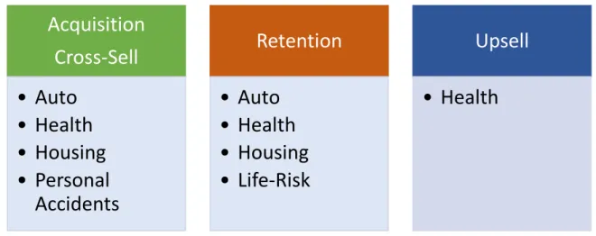
The Bank and the Insurance Company decided to have the NBAs focusing on the four major LoBs: Auto, Health, Housing and Personal Accidents (with Personal Accidents not being used for Churn-related actions and being substituted by Life-Risk), making the following actions available for NBA 1.0:
1. Acquisition of Auto Insurance 2. Acquisition of Health Insurance 3. Acquisition of Housing Insurance
4. Acquisition of Personal Accidents Insurance 5. Retention of Auto Insurance
19 7. Retention of Housing Insurance
8. Retention of Life-Risk Insurance
In the NBA 2.0, one more action was introduced: Up-Selling – the practice of offering other or better goods or services to a customer who is already buying something (Cambridge University Press 2011) – for Health related insurance products, making the total number of actions raising to 9.
Figure 3.4 - Map of NBAs used in NBA 2.0
Acquisition
Cross-Sell
• Auto
• Health
• Housing
• Personal
Accidents
Retention
• Auto
• Health
• Housing
• Life-Risk
Upsell
• Health
16
3.3.2. NBA 1.0
As mentioned before, the first stage of the NBA framework – NBA 1.0 – was primarily defined by model scores built specifically for Insurance products.
The first step was to analyze the existing predictive models and evaluate their performance in a campaign setting. All the models which were built before this project were revisited and, if the Bank and the Insurance Company were satisfied with the model performance, these models would be used in the NBA 1.0 table. If the companies were not satisfied with the existing model or there was not a model for a specific LoB intended to be used in the NBA, it should be built before starting the calculation of the NBAs.
Considering all the actions that were defined by the companies, Table 3.1 summarizes all the existing models for Insurance campaigns:
Table 3.1 - Models built between the Bank and the Insurance Company for Insurance Products
Line of Business Acquisition/Cross-Sell Churn Upsell
Auto Built and used for campaign leads selection
Built and used for campaign leads selection
Built and not used for campaign leads selection
Health Built and used for campaign leads selection
Built and used for campaign leads selection
In progress
Housing Not built Built and not used for campaign leads selection
Not built
Personal Accidents Not built Not built Not built
Life-Risk Not built Built and used for campaign leads selection
Not built
After a meeting with the Bank and the Insurance Company it was defined that the Upsell model for Auto LoB was not going to be used because it was not a priority to be included in the NBA project and the Upsell model for the Health LoB would be included in NBA 2.0 since it was being built and used in a separate project.
The final NBA 1.0 table was composed by the 4 blocks of information: 1. General Information
17 - Bank Segmentation
- Insurance Company Segmentation 2. Policy Ownership Information
- Number of active policies - Types of LoBs owned 3. Model Scores
- Auto Acquisition Model - Health Acquisition Model - Housing Acquisition Model
- Personal Accidents Acquisition Model - Auto Churn Model
- Health Churn Model - Housing Churn Model - Life-Risk Churn Model 4. Next Best Action
- NBA1 - NBA2 - NBA3
- NBA1 Confidence Level - NBA2 Confidence Level - NBA3 Confidence Level
3.3.2.1.
Analyzing Existing Predictive Models
As seen on Table 3.1, six models were already built and four of them were being used to select leads for ongoing campaigns.
All models were analyzed but for the purpose of this report, the model used to predict the propensity to buy a Health Insurance product will be used as an example since it was the model with the most interesting approach.
Propensity Model to Buy Health Insurance
This model was developed in late 2017 and was being used to help selecting leads for ongoing campaigns for acquisition and cross-selling of Health Insurance products, using the Data Mining software SAS® Enterprise Miner which provides many proven machine learning algorithm in a high performance environment (Hall et al. 2014).
The model was extremely interesting to analyze due to its unique approach. The team who was in charge of its construction decided to divide the model into two models: a model to predict the probability of the ownership of a Health insurance product (hereby called Health Ownership Model) and a model to predict the actual probability of buying an insurance product (known as Health Model). The goal of this division was to predict the propensity to buy a Health policy of people with low
18 probability of having a Health policy elsewhere, in order to have a better campaign performance by offering a Health Insurance product to people who actually need one.
o Ownership Model
The goal of the model was to optimize campaign contacts by excluding Bank clients who probably already possess a Health policy in another company by analyzing the transactional behavior of clients with and without Health Insurance.
Table 3.2 - Human Health Business Activity Code (Institituto Nacional de Estatística 2007) 2-DIGIT CODE 3-DIGIT CODE 4-DIGIT CODE 5-DIGIT CODE BUSINESS ACTIVITY
86 Human Health Acitvities
861 8610 86100 Health Establishment with hospitalization 862 Ambulatory Clinical Pratice
8621 86210 Ambulatory General Practice 8622 86220 Ambulatory Specialized Practice 8623 86230 Dentistry and Ondontolgy Practice 869 8690 Other Health Related Activities
86901 Blood Test Laboratories 86902 Ambulance Activities 86903 Nursing Care Activities
The general idea was to identify differences between the Health transactions of these two types of clients to see if patterns could be found and used to distinguish the clients with Health insurance or not.
This transactional behavior was focused on transactions related to Health such as hospitals, clinics and pharmacies, using the Business Activity Code (CAE in Portuguese) of their transactions associated to these fields (Table 3.2).
19 The first step was to define the universe to use (Figure 3.5) and to analyze the behavior of these two groups in terms of transactions in Health:
Assuming Bank clients who bought Health Insurance recently did not have Health Insurance before, their Health transactions in the months prior to the purchase can be seen as the behavior of clients without Health Insurance;
Health transaction of Bank clients who bought Health Insurance in the past and still own it can mimic the behavior of clients with Health Insurance.
The main idea of this analysis was proven to be correct: clients with Health Insurance present more medical transactions, but of small value (indicating they were using the Health Insurance), and non-insured clients present lesser medical transactions, but having considerable higher values than the ones coming from insured clients (meaning they were not insured or they were not using their insurance).
To assign a probability for having Health Insurance, a decision tree was made with the variables created from medical related transactions.
o Health Model
As expected, the main goal of the model is model is to calculate the probability of a given client to buy Health Insurance.
There was no Health Insurance campaign before building the model, so the universe taken into consideration was all Bank clients that bought Health Insurance between March 2016 and March 2017 without advising from the Bank, meaning clients who bought Health Insurance proactively (Table 3.3).
Table 3.3 - Health Model Universe
The Bank Data Mining team already possess a monthly process where they build a table with thousands of variables that can be used for modelling that can be divided into 7 groups:
Transactionality (variables related to Bank transactions)
Liability (liabilities of the client to the Bank and to the Bank of Portugal) Rentability (indicators of the value of the costumer to the Bank)
20 Possession (information about product ownership in the Bank)
Segmentation (geo-demographic and segmentation information about clients) Insurance Company (coded variables received from the Insurance Company)
The team also have their own standard procedure when it comes to predictive modelling. After creating the target variable and selecting the desirable temporal window, from these thousands of variables, the most important ones will be selecting by calculating its worth, with a combination of 3 different methods:
R2 – used for numeric variables. Known as the coefficient of determinations, it measures the proportion of the variance in the target variable that is predictable from the independent variable (Steel and Torrie 1960). Ranging from -1 to 1, the highest the absolute value, the more correlated is the variable to the target (Cameron and Windmeijer 1997).
Chi2 – Like R2 it is a measure of goodness-of-fit applied to categorical variables, testing the relationship, if it exists, between the target and the independent variables, being very robust statistical (McHugh 2013).
Decision Tree – In decision tree building, the decision tree model is built by recursively splitting the training dataset based on a locally optimal criterion until all or most of the records belonging to each of the partitions bear the same class label (Du and Zhan 2002).
With the combination of the three methods, a composite indicator is calculated, and the top 25 variables are used for the modelling step.
As a standard practice modelling technique, the universe was subset in a balanced sample of 50/50, which means that half of the clients in the
sampled universe bought Health Insurance. This sampling technique is used to optimize the performance of the predictive models which sometimes underperform when facing an imbalanced sample and cannot find the right features to identify the target (Chawla 2010).
After selecting the 25 most correlated variables with the target, 4 machine learning algorithms are used to create a predictive model:
Decision Tree Neural Network Logistic Regression Model Ensemble
Their output was then analyzed with the
Model Ensemble being the chosen algorithm by presenting the best lift (1.98 out of a maximum of 2 since it’s a 50/50 balanced sample) the and area under the ROC curve (0.89).
Figure 3.6 - Cumulative Lift of Model Ensemble, Logistic Regression and Neural Networks models
21 Even though these statistics showed promising results, a backtesting evaluation is needed to confirm the performance of the Health Model. Using a balanced sample of 50/50, like in the training data, the selected model was applied to historical client data from December 2015 to February 2016. The predictive model scores were divided into percentile groups (Table 3.4) and the percentage of targets was calculated.
As expected (Figure 3.7), there is an increasing percentage of targets in the groups, with the greatest percentage belonging to the highest average probability (05 – Very High). This means the model is work properly with data outside of its training set and not underfitting (Hawkins 2004).
The results of the other models (Table 3.1) that were already built and were meant to be used in the NBA framework held similar results and the Bank and the Insurance Company agreed not to redo any of them.
Figure 3.7 - Backtesting results of the Health Model
Predictive Model Score Group Below Percentile25 01 – VERY LOW
Between Percentile25 and Percentile50 02 – LOW
Between Percentile50 and Percentile75 03 – MEDIUM
Between Percentile75 and Percentile90 04 – HIGH
Above Percentile90 05 – VERY HIGH
22
3.3.2.2.
Building New Predictive Models
Almost every needed model was built but there were two specific acquisition/cross-sell models that had to be constructed: Housing and Personal Accidents Insurance LoBs.
Both models were built and tested, but, similarly to the analysis of the existing predictive models (cf. chapter 3.3.2.1), the predictive model for the acquisition of Personal Accidents Insurance will be described in its extension.
o Personal Accidents Model
The main goal of this model was to estimate the probability of acquiring/cross-selling a Personal Accidents Insurance product of Bank clients, residing in Portugal. There was no ongoing campaign regarding this type of Insurance so, like the Health Model built by the Bank Data Mining Team, there was no distinction of clients, excluding only clients who had own this product in the past (Table 3.5). The timeframe of the training set was set from February 2017 to February 2018, being the historical data of March, April and May 2018 reserved for backtesting (Figure 3.8).
Figure 3.8 - Temporal window for the Personal Accidents Model
Table 3.5 - Personal Accidents Model Universe
As mentioned in the Health Model, the Data Mining Team of the Bank already utilizes a monthly process to get a snapshot table of thousands of variables from different sources, divided into 7 groups: Transactionality, Liability, Rentability, Relationship, Possession, and Segmentation from the Insurance Company.
23 Since time was short and the NBA 1.0 was meant to be concluded as soon as possible, an analogous process to one used to select variables used for the Health Model was implemented for the Personal Accidents Model.
By calculating the R2, the Chi2 and using a decision tree, 8 variables (Table 3.6) stood out as the “best” variables to use for modelling with the variable from the Liability group assuming the greatest relative importance (Figure 3.9) and the variable from the Relationship group showing the lowest relative importance.
Table 3.6 - Groups of Selected Variables
Figure 3.9 - Relative Importance of the Groups of Selected Variables of the Personal Accidents Model After selecting the 8 variables, the next step was to use ML
algorithms to find the best models to calculate the propensity to buy Personal Accidents Insurance. The total percentage of target clients was 1.6%, having 3.500 target clients in a universe of 250.000. So, intending to avoid overfitting and performance problems, an undersampling of the modelling universe was done by selecting all 3.500 target clients and performing a random sample from the remaining universe, making up a modelling sample of 7.000 clients with a percentage of target clients equal to 50% (Figure 3.10). After building the final modelling universe, the universe was divided in two different sets: a training set compromising 70% of the modelling universe with the remaining 30% forming the validation set. Dividing the modelling universe in different sets is a common practice in supervised learning with the validation
Group of Variables Number of Variables Relationship 1 Possession 1 Segmentation 2 Transactionality 3 Liability 1
24 dataset is used to give an estimate of model while tuning the model’s hyperparameters (like the number of hidden layers in a Neural Network) (Gareth et al. 2013).
With the training and the validation set defined, and analogously like in the Health Model, 4 ML algorithms were tested in SAS® Enterprise Miner:
Decision Tree Neural Network Logistic Regression Model Ensemble
By analyzing the fit statistics of the 4 different models, the Neural Network came up as the chosen model (Table 3.7). Even though the Model Ensemble and the Neural Network present the same value of Lift, the Area Under the ROC Curve is higher in the Neural Network and the MSE is lower. The Decision Tree was the model with the worst performance.
Table 3.7 - Fit Statistics of the Personal Accidents Models
Measure Neural Network Decision Tree Logistic Regression Model Ensemble
Mean Squared Error 0.18 0.25 0.18 0.19
Area Under ROC Curve
0.8 0.75 0.79 0.79
Lift 1.7 1.3 1.6 1.7
Focusing on the Neural Network, the ROC curve of both the training and the validation set showed to be extremely similar, demonstrating the model was well calibrated (Figure 3.11).
25 To make sure the model was performing “well” in untested data, backtesting was performed in data from March, April and May 2018. Since the results from the Neural Network seem robust, the backtesting was applied in unbalanced data where the average target percentage was 15%.
Similar to the Health Model backtesting, the tested individuals were divided into groups accordingly to the model score percentile (Table 3.4). As expected, the group with the highest average model score (05 – Very High) presented the biggest percentage of target clients (with a lift of 3 comparing with the average target percentage in the backtesting group).
The backtesting also indicated the Neural Network has similar performances in all months.
Figure 3.12 - Backtesting of the Neural Network in more recent data
3.3.2.3.
Calculating NBA and Confidence Levels
With all the 8 models built (4 acquisition/cross-sell models – Auto, Health, Housing and Personal Accidents – and 4 churn models – Auto, Health, Housing and Life-Risk) and evaluated, the calculation of the formula of the NBA came up as the next step.
Being the NBA 1.0 mostly based on model scores, the concept of the NBA calculations was relatively straightforward: compare scores within each client and assign NBA1, NBA2 and NBA3 to the three highest model scores, but a business problem appeared: if a client has a high propensity to buy Housing and also a high propensity to abandon their Health Insurance, even if it is slightly lower, the chances of the client churning is high so instead of offering a product, shouldn’t NBA1 be a retention action instead of a new insurance recommendation?
Just comparing the scores proved to be insufficient so a ranking system was also introduced: if the client is in risk of abandoning their policy (indicating by having a high churn model score), the first action should be a retention action even if the client shows a high propensity to buy new products.
26 Besides assigning a hierarchy between retention and offering actions, in case of a tie in model scores for the same type of action, the first product to be shown should depend on business objectives (sometimes during certain campaigns, some products have bigger objective goals than others). To accommodate these settings, the calculation of the NBA is done by a system of transforming each action model score in a 5-digit number (Figure 3.13) and then finding the maximum number of all the model score numbers and assign it as the NBA:
The first digit is the priority of the action
o 9 for retention actions (if the model score is high) and 8 for offering actions and retention actions (if the model score is low)
The three middle digits are the first digits of the multiplication of the model score by 1000 The last digit is given depending on the priority of the product (and can be arranged depending
on the objectives of the ongoing campaigns)
Figure 3.13 – NBA 1.0 Formula
If the predictive models assign a customer who already possesses a Health Insurance product a score of 0.84513 for Auto Acquisition, 0.12598 for Housing Acquisition, 0.35698 for Personal Accidents Acquisition and 0.81549 for Health Churn, the calculation of the NBAs should be as followed, assuming the ongoing campaigns had a business pressure for selling more Auto Insurance, followed by Health, Housing and Personal Accidents Insurance:
Model Model
Score
Priority of Action Model Score X 1000 Hierarchical Product Priority NBA calculation number Order of NBA
Auto Acquisition 0.84513 8 845.13 9 88459 NBA2
Housing Acquisition 0.12598 8 125.98 7 81257 NBA3
Personal Accidents Acquisition 0.35698 8 356.98 6 83566 NBA4
Health Churn 0.81549 9 (high score) 815.49 8 981549 NBA1
27 Although the score for the Health Churn Model was not the highest, but was still considerably high, this method of calculations makes sure that a Health Retention Action would be NBA1 followed by the highest acquisition scores, making Auto Acquisition the NBA2 and Housing Acquisition the NBA3. With this transformation system, the way to calculate each client’s NBAs becomes quite easy to understand and implement but a new question arises: how confident are we that the NBA is really the next best action?
To address this question, both Data Mining Teams of the Bank and the Insurance Company reunited with me to discuss how to calculate the confidence of each action. After a brainstorm of several ideas, the Data Mining Team of the Insurance Company came up with a concept they had used in the past to compare model scores and that it could be applied to the NBA and be used as a confidence measure: lift-adjusted standardized probability.
The main idea of this measure is to standardize the model scores of each client by subtracting the average model score of the population and dividing it by its standard deviation and then adjusting it by multiplying the standardized score with the model lift to make sure that models which are proven to have a better performance assume higher values (Figure 3.14).
Figure 3.14 - Confidence Formula
With this new measure, confidence levels can be created by dividing the clients in groups according to their confidence percentile:
Confidence Percentile Confidence Level Below Percentile20 01 – VERY LOW
Between Percentile20 and Percentile40 02 – LOW
Between Percentile40 and Percentile60 03 – MEDIUM
Between Percentile60 and Percentile80 04 – HIGH
Above Percentile 80 05 – VERY HIGH
Table 3.9 - Confidence Levels
With the NBA and confidence formulas created the first phase reached an end and NBA 1.0 was completed.