Object detection for single tree species identification with high resolution aerial images

OBJECT DETECTION FOR SINGLE TREE SPECIES

IDENTIFICATION WITH HIGH RESOLUTION AERIAL IMAGES

OBJECT DETECTION FOR SINGLE TREE SPECIES

IDENTIFICATION WITH HIGH RESOLUTION AERIAL IMAGES

Dissertation supervised by

Joel Dinis Baptista Ferreira da Silva, PhD

Instituto Superior de Estatística e Gestão de Informação, Universidade Nova de Lisboa

Lisbon, Portugal

Dissertation co-supervised by Pedro da Costa Brito Cabral, PhD

Instituto Superior de Estatística e Gestão de Informação, Universidade Nova de Lisboa

Lisbon, Portugal

Dissertation co-supervised by Filiberto Pla Bañón, PhD

Institute of New Imaging Technologies, Universitat Jaume I

Castellón de la Plana, Spain

D

ECLARATION OF

O

RIGINALITY I declare that the work described in this document is my own and not from someone else. All the assistance I have received from other people is duly acknowledged and all the sources (published or not published) are referenced. This work has not been previously evaluated or submitted to NOVA Information Management School or elsewhere.

Lisbon, 17.02.2020

Ekanayaka Mudiyanse Ralahamilage Chamodi Lakmali Boyagoda [the signed original has been archived by the NOVA IMS services]

A

CKNOWLEDGMENTS

I dedicate this paragraph to express my gratitude to persons who helped me to complete my master thesis successfully. Firstly, I would like to express my sincere gratitude to my supervisor Dr. Joel Silva for his continuous knowledge sharing and guidance during master thesis. Secondly, I would like to thank my co-supervisors Prof. Dr. Pedro Cabral and Prof. Dr. Filiberto Bañón for their valuable feedback. Special thank goes to Prof. Marco Painho and Dr. Christoph Brox for their support and guidance throughout the master program. I would like to extend my gratitude to all professors for helping me improve my knowledge on the subject area. Finally, I express my gratitude, love, and respect to my family and friends for their encouragement and support.

OBJECT DETECTION FOR SINGLE TREE SPECIES

IDENTIFICATION WITH HIGH RESOLUTION AERIAL IMAGES

A

BSTRACT

Object recognition is one of the computer vision tasks developing rapidly with the invention of Region-based Convolutional Neural Network (RCNN). This thesis contains a study conducted using RCNN base object detection technique to identify palm trees in three datasets having RGB images taken by Unnamed Aerial Vehicles (UAVs). The method was entirely implemented using TensorFlow object detection API to compare the performance of pre-trained faster RCNN object detection models. According to the results, best performance was recorded with the highest overall accuracy of 93.1 ± 4.5 % and the highest speed of 9m 57s from faster RCNN model which was having inceptionv2 as feature extractor. The poorest performance was recorded with the lowest overall accuracy of 65.2 ± 10.9% and the lowest speed of 5h 39m 15s from faster RCNN model which was having inception_resnetv2 as feature extractor.

K

EYWORDS

Convolutional Neural Network High Resolution Aerial Images Image Classification

Object Detection

Region-based Convolutional Neural Network Remote Sensing

A

CRONYMS

AI – Artificial Intelligence

CNN – Convolutional Neural Network DEM – Digital Elevation Model

IoU – Intersection over Union ML – Machine Learning

NDVI – Normalized Differential Vegetation Index NMS – Non-Maximum Suppression

OBIA – Object Based Image Analysis

RCNN – Region-based Convolutional Neural Network

RF – Random Forest

RGB – Red Green Blue RoI – Region of Interest

RPN – Region Proposal Network SSD – Single Shot Detector SVM – Support Vector Machine UAV – Unmanned Aerial Vehicles YOLO – You Only Look Once

I

NDEX OF THE

T

EXT

DECLARATION OF ORIGINALITY ... III ACKNOWLEDGMENTS ... IV ABSTRACT ... V KEYWORDS ... VI ACRONYMS ... VII INDEX OF THE TEXT ... VIII INDEX OF TABLES ... X INDEX OF FIGURES ... XI

1. INTRODUCTION ... 1

1.1 An overview of the work ... 1

1.2 Objectives ... 3

1.3 Dissertation Organization ... 3

2. LITERATURE REVIEW ... 4

2.1 Identification of Tree Species with High Resolution Aerial Images ... 4

2.1.1 Applications in Agriculture and Crop Management ... 4

2.1.2 Applications in Forestry Management ... 5

2.2 Applications of Object Detection ... 6

2.3 Object Detection with Convolutional Neural Network (CNN) ... 7

2.4 Object detection with R-CNN ... 9

2.4.1 Region proposals ... 9 2.4.2 Feature extraction ... 10 2.4.3 Classifier ... 10 2.4.4 Evolution of RCNN Family ... 11 3. THEORETICAL BACKGROUND ... 12 3.1 Faster RCNN Architecture ... 12

3.2 Pre-trained CNN (Feature Extractor) ... 12

3.2.1 Inception V2 ... 13

3.2.2 Resnet 50 and Resnet 101 ... 14

3.3 Region Proposal Network (RPN) ... 16

3.3.1 Anchors ... 17

3.4 Region of Interest (RoI) Pooling ... 17

3.5 RCNN ... 18

3.6 Training ... 18

4. DATA AND METHOD ... 20

4.1 Data Description ... 20

4.2 Method ... 21

4.2.1 Tools ... 22

4.3 Pre-processing & labelling ... 23

4.4 Training object detection models ... 24

4.5 Testing trained models ... 24

4.6 Accuracy assessment ... 25

5. RESULTS ... 26

5.1 Image pre-processing & labelling ... 26

5.2 Training object detection models ... 28

5.3 Testing trained models ... 28

5.4 Accuracy assessment ... 30 6. DISCUSSION ... 33 7. CONCLUSIONS ... 37 BIBLIOGRAPHIC REFERENCES ... 38 ANNEX I ... 42 ANNEX II ... 46

I

NDEX OF

T

ABLES

Table 1: Architecture of Inception v2 feature extractor (Ioffe and Szegedy, 2015) ... 14

Table 2: Detail architecture of Resnet 50 and Resnet 101(He, 2015). ... 15

Table 3: Number of images in train, validation and test data for each dataset ... 26

Table 4: Number of bounding boxes extracted from cropped images ... 27

Table 5: Total time duration for training and validation of each model... 28

Table 6: Evaluation results of dataset 1 for faster_rcnn_inception_v2 model ... 31

Table 7: Summary of evaluation results for each model per dataset. The values represent mean ± standard deviation ... 31

I

NDEX OF

F

IGURES

Figure 1: Layer arrangement of neural network (Karpathy, 2019) ... 8

Figure 2: Overview of object detection system (Girshick et al., 2016) ... 9

Figure 3: Faster RCNN architecture (Rey, 2018) ... 12

Figure 4: Convolutional layer arrangement of inception module (Szegedy et al., 2016)13 Figure 5: A block of 3 layers with shortcut connection (He, 2015). ... 14

Figure 6: Detail architecture of Inception Resnet v2 (Szegedy et al., 2017) ... 16

Figure 7: RPN architecture (Ren et al., 2017) ... 17

Figure 8: RoI pooling implemented on a proposal (Rey, 2018) ... 18

Figure 9: RCNN architecture (Rey, 2018) ... 18

Figure 10: Methodology Flowchart ... 21

Figure 11: Examples of cropped images. ... 26

Figure 12: Example of labelled image from dataset 1 ... 27

Figure 13: Total loss vs steps graph of faster_rcnn_inception_v2 model for Dataset 1 ... 28

Figure 14: Classified images from faster_rcnn_inception_v2 model ... 29

Figure 15: Evaluation results of classified images from faster_rcnn_inception_v2 model ... 30

1. I

NTRODUCTION

1.1 An overview of the work

Identification of tree species presented in the environment has a vital importance in assessing biodiversity, monitoring the behavior of invasive species, urban planning, agriculture and crop management, forest management and monitoring wildlife habitat (Steele, 2016). Among them forests are the most precious natural resource on Earth to be managed effectively since their contribution in the consistence of the ecological balance (Torahi and Rai, 2011). Maintaining forest inventories is a key factor of sustainable forestry management where it reveals more information about the forests such as composition of tree species, population of trees and health, making it easy to take decisions (Chiang, Valdez and Chen, 2016). For an example, forestry officer may need to identify invasive tree species and remove them to maintain the health of other trees. Field investigations for such purposes often involve time and labor consuming costly procedures due to many reasons such as safety issues and forest are located remotely making it difficult to access (Chiang, Valdez and Chen, 2016). Maintaining reliable and accurate forest inventories is a cost-effective approach to handle such situations. On the other hand, not only in forest, surveying to obtain tree population in urban planning is also labor intensive and time consuming (Perkins, 2016).

In such cases, it is highly effective to take benefits from remote sensing techniques. Classifying trees to identify tree species from remotely sensed images would be an ideal solution to above issues. The concept is being widely applied to sustainable management of large-scale crop field with having different types of crops.

Nowadays, remotely sensed images can be acquired by two different ways. One is to conduct aerial survey using Unmanned Aerial Vehicles (UAV) with on

board camera. The other way is to obtain from satellites. High resolution images are more applicable since the main purpose is to identify tree species.

Since the main target is to detect objects specially trees, the most appropriate image processing techniques is Object-Based Image Analysis (OBIA). OBIA involves categorization of image objects which are having similar set of pixels in terms of spectral properties such as color, size, texture and shape (Humboldt State University, 2019). Convolutional Neural Networks (CNNs) are fast growing technology among researchers which have the capability of object recognition with high accuracy and less human intervention (Guirado et al., 2017). Guirado et al. (2017) has proven that CNN based image recognition methods provides quite promising results over the other OBIA methods. Furthermore, CNNs are widely used in object recognition tasks as feature extractors aiming to feed those information in machine learning models to classify images (Olivares, 2019).

With the advancement of Artificial Intelligence (AI), plenty of researches have been conducted to evaluate the use of Machine Learning (ML) techniques to optimize and improve the quality of classification process. In remote sensing, labelled data are used to train such ML algorithms so that it can be utilized to determine the labels of unclassified data (Shetty, 2018). First and most remarkable development in object recognition is the introduction of Region-based Convolutional Neural Network (RCNN) which connects CNN with Support Vector Machine (SVM) by Girshick et al., 2016.

This thesis is basically focused on identifying Palm trees in high resolution aerial images by identifying trees as objects using pre-trained object detection models which are having RCNN architecture. The process is assuming that the variation in spectral signatures between species and texture are adequate to distinguish Palm trees from other species. This will be an attempt to prove the capability of recently developed object detection technique RCNN in agricultural field. Unlike the previous methods used to detect trees using expensive multispectral images with CNN which requires thousands of training images, the

method proposed by this thesis uses only less amount of RGB images with use of pre-trained RCNN object detection models.

1.2 Objectives

The main objective of the study is to identify single tree species presented in high resolution aerial images using RCNN based object detection techniques. Following specific objectives are identified to achieve the main objective;

• Evaluate the performance of pre-trained object detection models to identify Palm trees in high resolution images

• Compare several pre-trained object detection models to find out the best model for identifying Palm trees.

1.3 Dissertation Organization

The thesis consists of seven chapters. Chapter 1 describes the overview of the work including problem, motivation and objectives. Chapter 2 contains the summary of related work. Chapter 3 contains the theoretical background of the study. Chapter 4 illustrates the data and methodology implemented for identifying Palm trees. Chapter 5 explains the results of the experiments conducted. Chapter 6 contains a detailed discussion. Chapter 7 summaries and concludes on the findings of the research.

2. L

ITERATURE

R

EVIEW

This section consists of descriptions of high resolution images, previous studies carried out using CNN and high resolution images related to agricultural and forestry field, introduction to object detection, use of CNN in object detection and introduction to RCNN.

2.1 Identification of Tree Species with High Resolution

Aerial Images

Images acquired by digital cameras mounted on UAVs are getting famous in forestry and agriculture mapping due to high spatial resolution ranging from 2.5cm to 90cm (Safonova et al., 2019). Nonetheless, improvements in sensor technology in past decades have given earth observation satellites the ability to obtain high resolution images ranging from 30cm to 50cm (Id, Leng and Liu, 2018). Applications of remote sensing technologies in various fields including agriculture and forestry industry often get benefits from high resolution aerial images since they have a positive impact on the classification accuracy (Id, Leng and Liu, 2018). In addition, its ability to link them with recent improvements of ML techniques has motivated researches to develop new methods for analysis (Safonova et al., 2019). Previous studies attempting to identify tree species using high resolution images directs towards agriculture/crop management and forestry management.

2.1.1 Applications in Agriculture and Crop Management

Training samples derived from high resolution images have the potential to increase the accuracy when classifying low resolution satellite images for large scale mapping (Nomura, 2018). In Nomura (2018), seven similar crop types were identified with 95% accuracy using Sentinel-2 images together with training samples derived from high resolution images using Random Forest (RF) Classifier. Although, tree types were not clearly distinguishable in Sentinel-2

images, high accuracy may be achieved by incorporating all bands in the classification (Nomura, 2018).

More crowded overlapping oil plam tree crowns can be detected and counted with high resolution multispectral satellite images by training a CNN using thousands of manually labelled samples (Li et al., 2017). In Li et al. (2017), around 9000 samples were used to achieve 96% accuracy of detection with optimum parameter settings as number of kernal in two convolution layers as 30 and 55 and number of hidden units in fully-connected layer as 600. In Csillik et

al. (2018), similar accuracy was achieved in identifying citrus trees by training

CNN using thousands of training samples derived from UAV multispectral images. Classification accuracy can be improved by applying object-based post processing with results from CNN (Csillik et al., 2018).

In Olivares (2019), it is proposed a method to classify UAV images to detect palm trees with reduced number of training samples using pre-trained CNN. However, due to the input size constrain in CNN based feature extractor the detection of induvial palm trees were not possible (Olivares, 2019). The model showed less performance in identifying target tree when it is surrounded by other tree types.

2.1.2 Applications in Forestry Management

Remote sensing takes advantage when discriminating tree species from aerial images from the fact that trees share unique spectral signature depending on the type of species they belong to (Lisein et al., 2015). However, spectral signature within and between species changes temporally. In Lisein et al. (2015), it was discovered that the optimal phenological time window for discriminating broadleaved trees lies between late spring and early summer (the end of leaf flushing). During this period, the intra-spectral variation within tree species minimizes while maximizing inter-spectral variation between species (Lisein et

of field mapping to input them in automatic object-based supervised RF classifier to identify five tree species based on spectral variation.

In Onishi and Ise (2018), it has been exposed in their study that deep learning can distinguish seven tree species with 89.0 % accuracy using individual tree crowns segmented from basic RGB UAV image of forest. This method has benefits in both performance-wise and cost-wise over previous methods which used expensive multispectral images (Onishi and Ise, 2018). However, his model’s accuracy depends highly on the number of training samples per each class and the quality of tree crown segmentation. Although DEM and slope models have been incorporated with increased number of training samples, misclassifications have resulted due to imperfect segmentation.

In Safonova et al. (2019), it has also been proved that CNN based classification models have potential to identify four damage stages of Fir trees with an accuracy of 99.7% based on the shape, texture and colour of tree crown in UAV RGB images of mixed forest. Increasing the volume of samples by data augmentation techniques can substantially improve the accuracy of classification when there is relatively small training dataset (Safonova et al., 2019). Although candidate selection technique was adopted to find regions of potential crowns in the image before feeding them in CNN, some misclassifications were resulted.

In fact, identifying8 individual tree crowns using only RGB bands is a difficult tasks specially in dense foressts which may be requiring more information such as multispectral bands, NDVI or other spectral indices and 3D LIDAR data (Safonova et al., 2019). Combining small amount of hand annotated high quality tree crwon training data with a large amount of tree crowns auto-generated from LIDAR data by unsupervised algorithm can be used to train CNN to identify individual trees (Weinstein et al., 2019).

2.2 Applications of Object Detection

Object detection is a combination of computer vision tasks image classification and object localization to classify and locate the presence of objects

in an image (Brownlee, 2019). Image classification comprises of algorithms to predict the class of one object in an image. Object localization comprises of algorithms to locate one or more objects present in an image by drawing bounding boxes around them. Accordingly, object detection comprises of algorithms to locate the presence of one or more objects in an image by drawing bounding boxes with labels indicating their class or type of category. These three computer vision tasks are generally referred to as object recognition (Brownlee, 2019).

Applications of object detection techniques are visible in various industries such as vehicle detection and counting in transportation industry, building detection in urban planning, face detection and people counting in security purposes and animal monitoring and counting in livestock management. Although ML is widely using in agriculture and forestry industry, a very few studies have been focused on using object detection. ML applications in crop management are found in yield prediction, disease detection, weed detection and species recognition (Liakos et al., 2018).

In Arsenovic et al. (2019), object detection was applied to identify diseased leaves in high resolution images proving its capability for the task over traditional ML techniques. Pre-trained object detection models such as Faster RCNN, SSD and YOLOv3 can successfully detect diseased leaves even in complex backgrounds at high accuracy (Arsenovic et al., 2019).

2.3 Object Detection with Convolutional Neural Network

(CNN)

The most straightforward approach is detecting objects using CNN which is widely used deep learning algorithm in image classification (Sharma, 2018). The following section explains the CNN based on the Stanford University lecture series on CNNs for Visual Recognition (Karpathy, 2019).

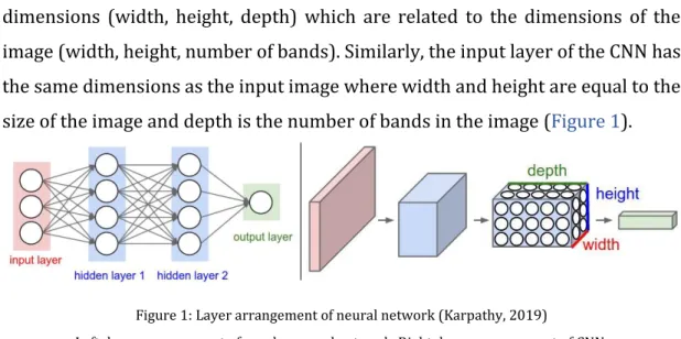
CNN differs from regular neural networks as it explicitly assumes that the inputs are images. In this way layers in CNN have neurons arranged in three

dimensions (width, height, depth) which are related to the dimensions of the image (width, height, number of bands). Similarly, the input layer of the CNN has the same dimensions as the input image where width and height are equal to the size of the image and depth is the number of bands in the image (Figure 1).

CNN architecture consists of three types of layers; convolutional layers, pooling layer and fully connected layer. Convolutional layers have small spatial filters which convolve across the width and height of input volume computing the dot product between pixel values of the filter and input image at each position during the forward pass resulting a two-dimensional activation map for each filter. This filter shifts over the original image by certain number of pixels called stride. When the stride is one, then the filter shifts by one pixel at a time. After every convolutional operation, non-linear operation called Rectified Linear Unit (ReLU) is introduced to replace negatives values in the feature map to zero. Pooling layers are inserted in between convolutional layers to reduce the spatial size and computational complexity in the network. This is generally done by sliding a filter across the width and height of the input while taking the maximum within the filter which is called as Max pooling. Fully connected layer has all neurons fully connected to the previous layer. It is a Multi-Layer Perceptron using a softmax activation function which keeps the output value ranging from 0 to 1. Once an image is passed through convolution and pooling layers of CNN, it predicts the class of the object in the image as output. Original image is divided into small tile and each tile is fed to CNN so that it predicts the class of each input tile. Later, classified tiles are combined to obtain the classes of all objects in the

Figure 1: Layer arrangement of neural network (Karpathy, 2019)

original image (Sharma, 2018). This kind of straightforward application of CNN requires all objects to share a common aspect ratio (Girshick et al., 2016). Hence, this approach contains problems as objects in an image has different aspect ratios and spatial locations. It is required to utilize thousands of such tiles to overcome that problem resulting more computational time (Sharma, 2018). In Girshick et

al. (2016), it is proposed a method called RCNN to address the above problems.

2.4 Object detection with R-CNN

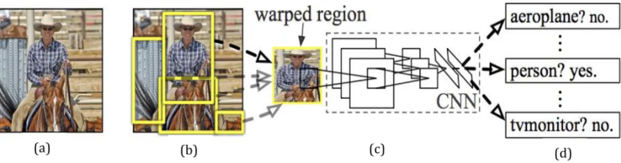
Following section describes the architecture of object detection system proposed by Girshick et al., 2016. It has been recognized as the first and most successful CNN approach addressing problems related to object localization, detection and segmentation (Brownlee, 2019). RCNN consists of three modules. They are region proposal, feature extractor and classifier. Region proposals generate category independent regions to consider for feature extraction. Feature extractor extract fixed length vector from each region using CNN. Third module classifies each region into one of the known classes using linear SVM model. The Figure 2 illustrates the overview of object detection system proposed by Girshick et al., 2016.

2.4.1 Region proposals

In RCNN, category independent region proposals are generated using selective search method (Girshick et al., 2016). Region proposals are bounding

Figure 2: Overview of object detection system (Girshick et al., 2016)

(a) It takes image as input. (b) around 2000 region proposals are generated. (c) features are computed for each proposal region using CNN. (d) Each region is classified using class specific linear SVM model

boxes representing potential objects in an image. Selective search technique proposes Region of Interest (ROI) by recognizing patterns based on the varying scales, colours, textures, and enclosure in the image (Sharma, 2018). Image is initially divided into small segments and combined them to obtain large segments taking into consideration of similarities of scale, colour and texture etc (Sharma, 2018).

2.4.2 Feature extraction

Features are the crucial factor in ML modelling techniques which are responsible for generating effective solution when as much as information is extracted from targeted dataset (Dey, 2018). Generally, CNN having architecture of convolutional and pooling layers acts as feature extractors which can be used to extract features before introducing them into ML models such as SVM, RF, etc. (Perone, 2015). Most cases, pre-trained CNNs are utilized as feature extractors by removing last output layer where the process is called transfer learning (Perone, 2015). The features extracted by pre-trained CNN have potential to train ML models to perform classification on very high resolution images (Olivares, 2019).

In RCNN, fixed length feature vectors are extracted from each region proposal using CNN developed by Krizhevsky, Sutskever and Hinton, 2012. CNN accepts fixed size of images as input (Girshick et al., 2016). Therefore, pixels surrounded by bounding box of region proposal are warped to get 227 x 227 pixel size image before feeding them into CNN. Input images are passed through five convolutional layers and two fully connected layers.

2.4.3 Classifier

After extracting features, regions are classified into known classes using linear SVM. One SVM is trained for each known class by applying extracted features with training labels during the training phase. The performance of the model becomes higher when involving SVM for classification rather than getting the output from last layer of fine-tuned CNN (Girshick et al., 2016).

2.4.4 Evolution of RCNN Family

However, RCNN possesses few drawbacks such as multi-stage training process requiring operation of separate models, requiring a storage of hundreds of gigabytes and slow object detection due to the extraction of features from each region proposal in image (Girshick, 2015). Fast RCNN was introduced to address those issues by reducing training stages to single pipeline. Although, it was fast than RCNN it still requires CNN to pass through region proposals for each image (Girshick, 2015). Faster RCNN which is described in next chapter, is a further improved version to obtain fast and accurate detection model.

3. T

HEORETICAL

B

ACKGROUND

Previous chapter provides an introduction to RCNN. This chapter extensively explains the faster RCNN architecture and feature extractors used in the method proposed in this thesis.

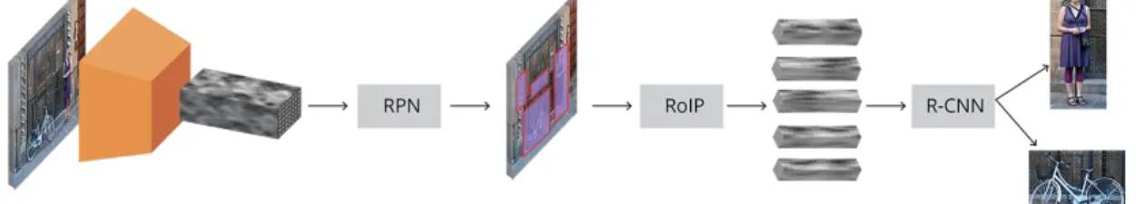
3.1 Faster RCNN Architecture

Faster RCNN is an integrated network which shares a deep fully convolutional network known as RPN with state-of-the-art object detection network known as Fast RCNN (Ren et al., 2017). It comprises of four modules namely Pre-trained CNN, RPN, ROI pooling and RCNN as illustrated in Figure 3.

Figure 3: Faster RCNN architecture (Rey, 2018)

First step is to generate a convolutional feature map from a tensor (multidimensional array) of input image which is fed into a pre-trained CNN. In RPN, predefined number of regions which contain objects are proposed by using fixed sized reference bounding boxes called anchors which are placed on feature map. RoI pooling is applied to extract features of relevant objects (bounding boxes proposed by RPN) from feature map computed by pre-trained CNN. RCNN classifies the object into a class and adjust the bounding box coordinates (Rey, 2018).

3.2 Pre-trained CNN (Feature Extractor)

Faster RCNN originally used output of an intermediate layer of VGG which is a CNN trained to classify ImageNet dataset to extract features from input image. It takes the output of convolutional layers by learning edges, patterns and shapes of objects resulting a convolutional feature map of input image which has smaller

spatial dimensions with greater depth than original image (Rey, 2018). Although ZF and VGG were considered as deep networks, much deeper networks have been invented after them. Such networks known as Inception v2, Resnet 50, Resnet 101 and Inception resnet v2 which were used in the study are explained below.

3.2.1 Inception V2

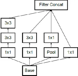
Inception v2 was presented by improving previous version to increase accuracy and reduce computational complexity. Accuracy has been improved by avoiding dimension reduction of input which may lead to loss of information and computational complexity has been reduced by factorizing 5x5 convolution layer to two 3x3 convolution layers (Szegedy et al., 2016). The layer arrangement of inception module is illustrated in Figure 4.

Figure 4: Convolutional layer arrangement of inception module (Szegedy et al., 2016)

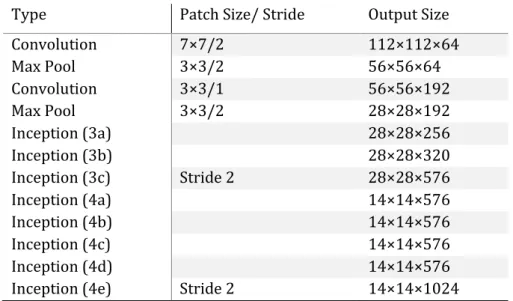
Inception v2 consists of several convolutional and pooling layers with a softmax layer for the final classification (Ioffe and Szegedy, 2015). In faster RCNN inception v2 model, end point has been set to inception (4e) layer for inception v2 to act as a feature extractor. Architecture of inception v2 feature extractor used in the experiment is illustrated in Table 1 assuming input is having spatial dimensions of 224x224.

Type Patch Size/ Stride Output Size Convolution 7×7/2 112×112×64 Max Pool 3×3/2 56×56×64 Convolution 3×3/1 56×56×192 Max Pool 3×3/2 28×28×192 Inception (3a) 28×28×256 Inception (3b) 28×28×320 Inception (3c) Stride 2 28×28×576 Inception (4a) 14×14×576 Inception (4b) 14×14×576 Inception (4c) 14×14×576 Inception (4d) 14×14×576

Inception (4e) Stride 2 14×14×1024

Table 1: Architecture of Inception v2 feature extractor (Ioffe and Szegedy, 2015) 3.2.2 Resnet 50 and Resnet 101

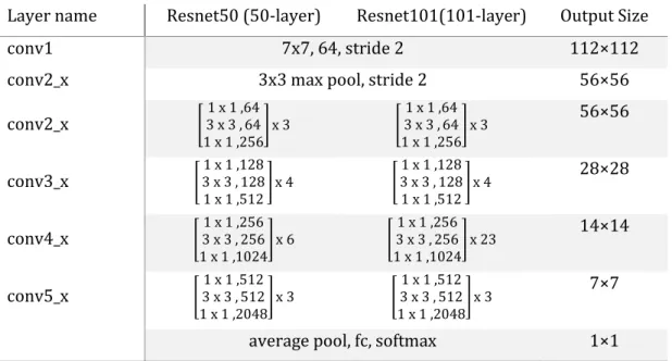
Residual networks have been developed by inserting shortcut connections to the plain networks which were inspired by VGG nets (He, 2015). Shortcut connections are inserted at each block as illustrated in Figure 5. Resnet 50 and Resnet 101 are built by block of layers consisting of 1x1, 3x3 and 1x1 convolutional layers. Detail architecture of Resnet 50 and Resnet 101 with number of blocks are summarized in Table 2.

Layer name Resnet50 (50-layer) Resnet101(101-layer) Output Size

conv1 7x7, 64, stride 2 112×112

conv2_x 3x3 max pool, stride 2 56×56

conv2_x [ 1 x 1 ,64 3 x 3 , 64 1 x 1 ,256 ] x 3 [ 1 x 1 ,64 3 x 3 , 64 1 x 1 ,256 ] x 3 56×56 conv3_x [ 1 x 1 ,128 3 x 3 , 128 1 x 1 ,512 ] x 4 [ 1 x 1 ,128 3 x 3 , 128 1 x 1 ,512 ] x 4 28×28 conv4_x [ 1 x 1 ,256 3 x 3 , 256 1 x 1 ,1024 ] x 6 [ 1 x 1 ,256 3 x 3 , 256 1 x 1 ,1024 ] x 23 14×14 conv5_x [ 1 x 1 ,512 3 x 3 , 512 1 x 1 ,2048 ] x 3 [ 1 x 1 ,512 3 x 3 , 512 1 x 1 ,2048 ] x 3 7×7

average pool, fc, softmax 1×1

Table 2: Detail architecture of Resnet 50 and Resnet 101(He, 2015). 3.2.3 Inception resnet V2

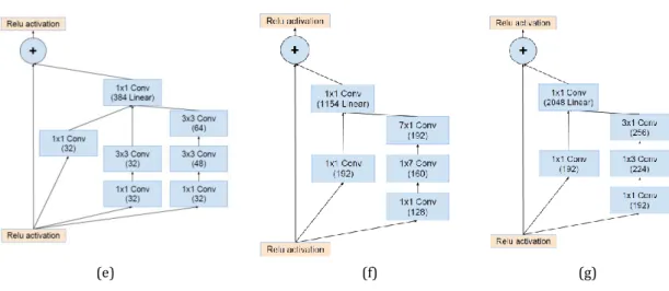
(a) (b)

(c)

(a) Schema for Inception-ResNet-v2; (b) The schema for stem of Inception-ResNet-v2 network; (c) The schema for 35 x 35 to 17 x 17 reduction-A module (k=l=256, m=n=384); (d) The schema for 17 x 17 to 8 x 8 grid-reduction-B module; (e) The schema for 35 x 35 grid Inception-resnet-A module; (f) The schema for 17 x17 grid Inception-ResNet-B module; (g) The schema for 8 x 8 grid Inception-ResNet-C module.

Inception resnet v2 has been proposed as a hybrid network which is inspired by resnet and inception v4 modules. Detail architecture is illustrated in

Figure 6. Residual connections have been inserted to add output from convolution layers of inception module to the input. 1 x 1 convolution layer has been inserted after each inception module as a filter expansion layer to avoid the dimensionality reduction occurred in inception block (Szegedy et al., 2017).

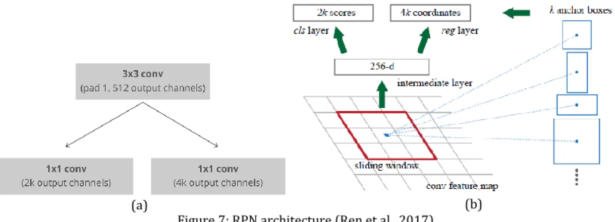
3.3 Region Proposal Network (RPN)

RPN is a fully convolutional network which takes all the reference bounding boxes known as anchors and outputs a set of rectangular object proposals with objectness score and bounding box coordinates (Rey, 2018). Objectness score represents the probability that an anchor is an object (Rey, 2018).

RPN is a small network having three convolutional layers as shown in

Figure 7 (a). 3 x 3 spatial window slides over the convolutional feature map to generate region proposals. Then the features from each sliding window are fed into two fully connected layers i.e. box regression layer and box classification

(e) (f) (g)

layer as illustrated in Figure 7 (b) (Ren et al., 2017). Classification layer outputs two scores for each anchor box being an object and a background. Regression layer outputs four coordinates of bounding box.

Figure 7: RPN architecture (Ren et al., 2017)

(a) Convolutional implementation of RPN architecture, where k is the number of anchors (Rey, 2018); (b) Sliding window at an anchor location (Ren et al., 2017)

3.3.1 Anchors

Anchors are predefined set of bounding boxes placed at each spatial position on convolutional feature map (Ren et al., 2017). Boxes with all possible combinations of three sizes i.e. 128px, 256px and 512px and three aspect ratios i.e. 1:1, 1:2 and 2:1 are defined per each anchor location (Ren et al., 2017). These boxes act as reference boxes to calculate and learn offsets when predicting bounding box locations (Rey, 2018).

3.4 Region of Interest (RoI) Pooling

RoI pooling takes the set of object proposals resulted from RPN and extracts fixed sized feature maps for each proposal so that they can be fed into RCNN to classify them into desired classes at the next step (Rey, 2018). This is done by cropping the convolutional feature map using each proposal. Cropped feature maps are resized into a fixed size usually 14 x 14 pixels and max polling is applied with a 2 x 2 kernel. Finally, it is ended up resulting a 7 x 7 feature map for each proposal as shown in Figure 8.

Figure 8: RoI pooling implemented on a proposal (Rey, 2018)

3.5 RCNN

Faster RCNN uses fast RCCN as its final module to classify those fixed sized feature maps resulted from RoI pooling. Two sibling fully connected layer are used to determine the class of the proposal with a score and adjust the bounding box coordinates to fit better as shown in Figure 9. One layer which has k+1 units outputs k object classes and background using a softmax function. The other layer which has 4k units outputs four values for corresponding k object classes to predict bounding boxes (Girshick, 2015).

Figure 9: RCNN architecture (Rey, 2018)

3.6 Training

RPN and RCNN are trained independently although they are designed to share common convolutional layers. RPN is trained by back propagation and stochastic gradient descent. All anchor boxes generated are categorized into two classes as positive and negative where if it is an object or background respectively. Anchor is labelled as positive if it has an IoU with any ground-truth boxes greater than 0.7. Anchor is labelled as negative if it has an IoU with all

ground-truth boxes lower than 0.3. Anchors do not have a label will not be considered for the training purpose. Non-maximum suppression (NMS) is applied to remove duplicate anchors that overlaps the same object (Ren et al., 2017). A batch of 256 samples having equal proportion of negatives and positives are randomly extracted from about 2000 anchors generated in RPN to compute classification loss and bounding box regression (Ren et al., 2017).

RCNN is trained similar to RPN. RCNN takes a batch of cropped features resulted from RoI pooling layer. A proposal is assigned to a ground-truth box if it is having an IoU greater than 0.5 with that ground-truth box. If IoU is between 0.1 and 0.5 with any ground-truth box, those proposals are labeled as background. Offsets of detected bounding boxes with ground-truth boxes are calculated for the boxes having a class. A batch of 64 samples are randomly selected to compute classification loss and bounding box regression (Rey, 2018).

4. D

ATA AND

M

ETHOD

This chapter contains the description of datasets used in this thesis followed by a detail explanation of proposed method to train object detection models and obtain metrices for each model.

4.1 Data Description

Three different datasets containing high resolution images acquired by UAVs were used in this thesis. These three datasets mostly contain palm trees and represent three different locations in Nicaragua, Tonga and Zanzibar. Tonga and Zanzibar datasets were downloaded from OpenAerialMap which is an open source platform for sharing imagery captured by openly licensed satellites and UAVs.

Dataset 1: The dataset prepared by Olivares, 2019 was used as Dataset 1.

It covers a palm tree plantation with an area of 45 ha. near Loma de Mico village in Municipality of Kukra Hill of Nicaragua. The data had been acquired by an aerial survey conducted on 27September 2014. The dataset possessed eleven RGB images of 3000 x 4000 pixels at a spatial resolution of 10 cm. Generally, the most prominent objects in the images are sparsely located and systematically distributed palm trees with the presence of dirt roads, small patches of natural forest and grasslands. Although, palm trees present in the images belong to different developing stages, only matured palm trees were considered for the analysis.

Dataset 2: The dataset consists of one RGB image covering Ha'akili and

Kolovai villages in Tongatapu Island of Tonga. It has been captured by Sony ILCE-6000 sensor mounted on UAV platform on 05 October 2017. The image is having dimensions of 17761 x 25006 pixels at a spatial resolution of 9 cm. The image comprises of areas where the palm trees are sparsely located as well as densely located with the presence of other trees, grasslands, bare land and houses.

Dataset 3: The dataset consists of one RGB image covering area between

Mangapwani and Bumbwini villages on Tanzanian island of Unguja, the main island of Zanzibar. It has been captured using UAV platform on 17 November 2016. The image is having dimensions of 38107 x 42858 pixels at a spatial resolution of 7 cm. The image comprises of areas where the palm trees are sparsely located as well as densely located with the presence of other trees, grasslands, bare land, roads and houses.

4.2 Method

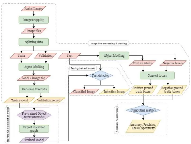
This thesis proposed a method to identify and locate palm trees by use of RCNN. The entire method consists of four major steps; image pre-processing and labelling, training object detection models for thesis datasets, testing trained models and accuracy assessment. Figure 10 illustrates complete process in step by step.

During pre-processing, original images were subjected to format conversion, cropping and objects labelling. Four pre-trained object detection models which are being trained to identify various objects were selected from TensorFlow object detection model zoo. They were trained using pre-processed thesis datasets. Accuracy assessment was conducted by comparing detection results from trained models. All steps were repeated for dataset 1, dataset 2 and dataset 3 separately. Detail explanation of each step is written in section 4.3 to

section 4.6.

4.2.1 Tools

This section lists out all the software and hardware which were utilized to implement the method proposed in section 4.2. The entire methodology was developed using open source software and packages.

• Anaconda is an open source distribution of python aiming to provide various packages and package management tools for scientific computing in data science and machine learning. Anaconda version 2019.07 was installed to manage programming environment for the project.

• Python is high level programming language which supports procedural, object-oriented and functional programming allowing users to write easy and logical codes. Python version 3.7.4 was installed inside Anaconda environment.

• TensorFlow is an end-to-end open source library for differentiable programming letting users to develop machine learning applications. It can be deployed in platforms likeCPUs, GPUs, and TPUs. TensorFlow CPU version 1.14.0 was installed inside Anaconda environment.

• TensorFlow Object detection API is an open source framework providing explicitly written collection of codes to build, train and deploy object detection models.

• LabelImg was used to label objects on image tiles. It is a graphical image annotation tool written in Python. Annotations are written into XML files in PASCAL VOC format used by Imagenet.

• Jupyter Notebook is an open-source web application that allows users interactive programming and visualization for scientific computing and data science applications. Jupyter Notebook version 6.0.1 was installed inside Anaconda environment.

• All processes were run on a laptop with an Intel i7-8550U CPU @ 1.99 GHz processor, 8 GB RAM and windows 10 64-bit operating system.

4.3 Pre-processing & labelling

The purpose of this step was to convert the original images into a form that is compatible with feeding them as input of pre-trained object detection models. TensorFlow object detection models only accept images in PNG/JPG format with three bands i.e. RGB (Huang et al., 2017). Since the original images were in TIF format, they were converted to JPG format using a python script which is attached in Annex II.

There is no size limit for the input images of TensorFlow object detection models since only intermediate layer (convolution layers) of pre-trained CNN feature extractor are being used (Rey, 2018). However, input images are resized to 600 x 1024 pixels in faster RCNN models keeping the aspect ratio of images constant to avoid the memory issues may arise during process (Ren et al., 2017). This size has been tested for NVidia Kepler GPU (Szegedy et al., 2016). Nevertheless, faster RCNN expects objects greater than 30 x 30 pixels. Since the average size of targeted objects is around 100 x 100 pixels, original images were cropped into tiles of 1000 x 1000 pixels to keep the size of objects greater than 30 x 30 pixels after resizing. Tiles which are not having palm trees were discarded. 10% of dataset was separated as test images and remaining dataset was split into 70% as train images and 30% as validation images.

Preparation of datasets for training: All objects (Palm trees) in train and validation images were labelled by drawing bounding boxes using LabelImg. Coordinates of bounding boxes and class were recorded in XML file for each image in the datasets. XML files together with corresponding images were converted to TFRecord format and generated train.record and validation.record files in order to feed them object detection models.

Preparation of datasets for accuracy assessment: All objects (Palm trees) in test images were labelled by drawing bounding boxes using LabelImg and coordinates were recorded into XML files. XML files were converted to CSV files and saved as positive ground truth boxes. Likewise, negative ground truth boxes were created by drawing bounding boxes in which palm trees were not presented.

4.4 Training object detection models

Four object detection models downloaded from TensorFlow object detection model zoo namely faster_rcnn_inception_v2, faster_rcnn_resnet50, faster_rcnn_resnet101, faster_rcnn_inception_resnet_v2 were trained providing train.record and validation.record prepared in section 4.3 as inputs. Training process was monitored using Tensorboard and terminated when the total loss reached value around 0.1. Inference graph of the model was exported after training was completed. This graph contains the weights of the trained model. Architecture of each model is described in chapter 3.

4.5 Testing trained models

Test images were fed into trained model resulted in section 4.4. Detection results were obtained into images in JPG format and coordinates of detection boxes were recorded in CSV file per each test image in dataset. The python script was run in Jupyter Notebook to test models and is attached in Annex II.

4.6 Accuracy assessment

Detection boxes were compared with corresponding positive ground truth boxes and negative ground truth boxes created as explained in section 4.3 to derive metrices; precision, Sensitivity, specificity and accuracy. It was based on the IoU calculated between detection boxes and ground truth boxes. Following definitions were defined for the calculation of metrices;

True positives (TP): detection boxes having IoU with positive ground truth boxes > 0.5

False positives (FP): detection boxes having IoU ≤ 0.5 or no intersection with positive ground truth boxes

False negatives (FN): ignored ground truth boxes

True negatives (TN): negative ground truth boxes having IoU ≤ 0.5 or no intersection with detection boxes

Following formulae were considered when computing metrices. Precision = TP

TP + FP

× 100

=

all positives correctly detected by model all positives detected by model

Sensitivity = TP

TP + FN

× 100

=

all positives correctly detected by model all positives in actual

Specificity = TN

TN + FP

× 100

=

all negatives correctly detected by model all negatives in actual

Accuracy = TP + TN

TP + FP + TN + FN

× 100

=

all correctly detected by model all in actual

5. R

ESULTS

This chapter consists of the outputs resulted from chapter 4. Only selected images are included in this chapter where appropriate. All other results are attached in Annex I.

5.1 Image pre-processing & labelling

Dataset 1 consisted of 49 tiles after cropping into 1000 x 1000 pixels of eleven RGB images of 3000 x 4000 pixels. Dataset 2 consisted of 283 tiles after cropping into 1000 x 1000 pixels of RGB image of 17761 x 25006 pixels. Dataset 3 consisted of 432 tiles after cropping into 1000 x 1000 pixels of RGB image of 38107 x 42858 pixels. Number of images after splitting dataset into train, validation and test data is summarized in Table 3. Example of cropped image for each dataset is shown in Figure 11.

Data Train Validation Test

Dataset 1 31 images 12 images 6 images

Dataset 2 179 images 76 images 28 images

Dataset 3 276 images 118 images 38 images

Table 3: Number of images in train, validation and test data for each dataset

Figure 11: Examples of cropped images.

(a) example of cropped images from dataset 1, (b) example of cropped images from dataset 2, (c) example of cropped images from dataset 3

Example of rectangular bounding boxes drawn using LabelImg is shown in Figure 12. Coordinates of each box recorded in XML file are in order of xmin, ymin, xmax and ymax.

Figure 12: Example of labelled image from dataset 1

(a) Example of labelled image from dataset 1, (b) showing a bounding box with coordinates

Labels were saved in XML file which contains coordinates of boxes with class. XML files were converted to CSV file format. Number of bounding boxes extracted are indicated in Table 4. The generated TFRecord files from CSV files and corresponding images comprise of numpy array of image with corresponding bounding box coordinates.

Data Train Validation Test

Palm tree Non- palm tree

Dataset 1 1996 765 441 101

Dataset 2 6121 2743 1240 517

Dataset 3 7158 3056 1433 678

Table 4: Number of bounding boxes extracted from cropped images

(xmin, ymin)

(xmax, ymax)

5.2 Training object detection models

Training process was terminated when the total loss becomes closer to 0.1. Total loss vs steps graph of faster_rcnn_inception_v2 model for Dataset 1 is shown in Figure 13. Total time durations including training and validation for each model with three datasets were recorded in Tensorboard and are summarized in Table 5. For dataset 1, frcnn_inceptionv2 model was the fastest and frcnn_resnet50 was slightly slower. For dataset 2, frcnn_resnet50 model was faster than other models. For dataset 3, frcnn_inceptionv2 model was the fastest. The frcnn_inception_resnetv2 model had the lowest speed for all three datasets. Overall, frcnn_inceptionv2 was the fastest model among others.

Model Dataset 1 Dataset 2 Dataset 3

frcnn_inceptionv2 19m 57s 29m 44s 9m 57s

frcnn_resnet50 20m 1s 19m 49s 19m 51s

frcnn_resnet101 50m 0s 59m 38s 29m 40s

frcnn_inception_resnetv2 5h 39m 15s 5h 0m 19s 5h 22m 51s

Table 5: Total time duration for training and validation of each model

5.3 Testing trained models

Trained model outputs each input image in which all detections are marked by rectangles with the name of class that object belongs to and confidence that

Steps T ot al lo ss

object belongs to identified class. Images in Test folder for each dataset were used to visualize the performance of each model. Such output images from faster_rcnn_inception_v2 model per dataset are shown in Figure 14. It can be seen that in Figure 14 (a), model was not capable of identifying all the objects (Palm trees) in the image. Figure 14 (b) is an example image where shadows of trees have been marked as Palm trees.

Figure 14: Classified images from faster_rcnn_inception_v2 model

(a) One of the classified images of Dataset 1; (b) One of the classified images of Dataset 2; (c) One of the classified images of Dataset 3

(a) (b)

5.4 Accuracy assessment

Images in the Test folder for each dataset were used to evaluate each model by computing precision, Sensitivity, specificity and accuracy. Total number of bounding boxes manually extracted to utilize as positive (palm trees) and negative (Non-palm trees) ground truth boxes are summarized in Table 4. Figure 15 (a) is an example image showing evaluation results of one of the images in Test folder of dataset 1. Similarly, Figure 15 (b) and (c) illustrate examples for dataset 2 and 3 respectively.

Figure 15: Evaluation results of classified images from faster_rcnn_inception_v2 model (a) Evaluation results of one of the classified images of Dataset 1; (b) Evaluation results of one of the

classified images of Dataset 2; (c) Evaluation results of one of the classified images of Dataset 3

(a) (b) (c) True positives False positives False negatives True negatives Legend

Table 6 lists all the evaluation results from faster_rcnn_inception_v2 model for images in test folder of dataset 1. Values in Table 6 was used to compute mean and standard deviation of precision, Sensitivity, specificity and accuracy for faster_rcnn_inception_v2 model. Accuracy measures for other models per each dataset also calculated in similar manner. Table 7 summarizes the mean and standard deviation values of each accuracy measures for all models per each dataset. Image TP FP FN TN image1 59 0 8 34 Image2 71 2 7 28 Image3 70 1 3 10 Image4 71 1 9 5 Image5 63 2 8 21 Image6 55 0 17 3

Table 6: Evaluation results of dataset 1 for faster_rcnn_inception_v2 model

Dataset Accuracy

measure _{inceptionv2 resnet50} Model _{resnet101 inception_resnetv2} Dataset 1 Precision 98.6 ± 1.2 98.2 ± 1.4 97.9 ± 2.0 98.3 ± 1.7 Sensitivity 88.1 ± 5.9 91.1 ± 3.3 90.7 ± 4.4 70.3 ± 10.2 Specificity 93.1 ± 5.8 89.4 ± 8.2 82.4 ± 20.4 94.1 ± 6.4 Accuracy 89.0 ± 5.7 91.4 ± 3.3 91.0 ± 3.3 74.2 ± 10.5 Dataset 2 Precision 96.1 ± 7.8 94.8 ± 7.5 88.8 ± 9.5 94.5 ± 10.2 Sensitivity 93.0 ± 5.1 86.9 ± 8.9 92.3 ± 5.4 49.9 ± 14.6 Specificity 94.1 ± 7.8 92.3 ± 8.1 81.7 ± 9.1 95.5 ± 6.1 Accuracy 93.1 ± 4.5 88.4 ± 7.1 87.9 ± 5.2 65.2 ± 10.9 Dataset 3 Precision 98.0 ± 3.0 97.8 ± 3.1 95.1 ± 4.9 98.8 ± 2.5 Sensitivity 83.7 ± 9.2 86.2 ± 8.6 80.7 ± 9.4 80.7 ± 10.5 Specificity 96.9 ± 4.8 96.7 ± 4.7 93.4 ± 5.5 98.5 ± 2.9 Accuracy 88.4 ± 6.6 89.9 ± 5.7 85.2 ± 7.0 86.9 ± 6.8 Table 7: Summary of evaluation results for each model per dataset. The values represent mean ±

standard deviation

Faster_rcnn_resnet50 model shows highest overall accuracy for both dataset 1 and dataset 3 with a value of 91.4 ± 3.3 % and 89.9 ± 5.7 % respectively.

Faster_rcnn_inceptionv2 model performance was the best for dataset 2 with an overall accuracy of 93.1 ± 4.5 %. However, the three models faster_rcnn_inceptionv2, faster_rcnn_resnet50 and faster_rcnn_resnet101 show similar performance for three datasets while faster_rcnn_inception_resnetv2 model depicts considerably lower performance for dataset 1 and dataset 2.

Figure 16 illustrates the accuracy, precision, sensitivity and specificity with standard deviation of each model. In Figure 16 (a) it is visible that dataset 1 and dataset 2 depict a similar behavior for four models. All four models resulted a high precision values for dataset 1 while lower precision values for dataset 2.

Figure 16: Graphs visualizes the differences in accuracy measures

(a) Accuray and standard deviation; (b) Precision and standard deviation; (c) Sensitivity (recall) and standard deviation; (d) Specificity and standard deviation

(a) (b)

6. D

ISCUSSION

This chapter contains a detailed explanation of the results and experiments conducted. This chapter also describes limitations of the study and recommendations for future works.

Image classification is one of the primary tasks in remote sensing which is vastly evolving with the improvements of machine learning techniques. Applications of image classification are mostly found in crop and forestry management (Liakos et al., 2018). Some of the applications of CNN in image classification tasks have been discussed in section 2.1. Those are few examples that proves the capability of deep learning base approaches specially CNN in remote sensing context. One of the common limitations of those methods is the requirement of a large number of training data to achieve better accuracy. Although, Olivares, 2019 proposed a method which requires reduced number of training samples, individual tree identification was not possible. Hence, this thesis proposed a method addressing the gap of previous methods with the use of object detection techniques.

The proposed method only utilizes high resolution RGB images taken by UAVs making it cost effective than using expensive data such as multispectral images, surface elevation models etc. All experiments were conducted using open source software. Use of pre-trained object detection models allowed to conduct image classification with a small number of training data. This justifies that transfer learning is feasible method for image classification tasks with small amount of data as mentioned by Olivares, 2019. The results of this thesis depict the capability of RCNN based object detection techniques to identify target even in complex backgrounds. Csillik et al., 2018 and Arsenovic et al., 2019 also showed that CNN and RCNN have the ability to perform well in complex surroundings.

The main reason behind the use of three datasets was to analyze the performance of each model for different scenarios. It helped to determine the behavior of each model when identifying same tree species in different surroundings, textures, sizes, color variations and spatial patterns. Dataset 1 contains systematically distributed regular sized palm trees with few numbers of smaller palm trees. Dataset 2 consists of regular sized randomly distributed palm trees with mostly affected by wind. Shadows of palm trees were also visible in dataset 2. Randomly distribute palm trees with variation in size indicating different growing stages were presented in dataset 3. In dataset 3, palm trees were surrounded by other tree types and at some locations palm trees were densely packed.

When carefully examining the detection results, it was found that the faster_rcnn_inceptionv2 model was not good at identifying small trees and trees located at the edges. But it performed well in distinguishing shadows of trees with target trees than other models. The faster_rcnn_resnet50 model performed well when the target trees were presented in different sizes. But it misidentified shadows as target trees. The faster_rcnn_resnet101 model produced better results when target trees are systematically distributed over the study area. The performance of faster_rcnn_resnet101 model became lower when the size of the target trees varies, and shadows were presented in the image. The faster_rcnn_inception_resnetv2 showed a poor performance when the orientation and texture of trees vary between one another. However, it performed well when the size of target trees varies.

Therefore, for dataset 1 and dataset 3, faster_rcnn_resnet50 model achieved higher overall accuracy while for dataset 2 faster_rcnn_inceptionv2 model achieved the higher value. Regardless of datasets, the highest overall accuracy was reached by faster_rcnn_inceptionv2 model and the lowest value was resulted by faster_rcnn_inception_resnetv2 model.

When considering the total time duration recorded for each model per dataset in Table 4, it can be decided that the speed of model depends on the

dataset. The frcnn_inceptionv2 model indicated the highest speed during the training process. This might be a result of computational efficiency of inception layers as the speed is directly affected by number of parameters and types of layers in the network (Huang et al., 2017).

According to the results in Table 6, it can be concluded that the performance of models depends on the dataset. The faster_rcnn_inceptionv2 model indicates high specificity and low sensitivity for dataset 1 and dataset 3 providing evidence of overfitting. But for dataset 2, it is perfectly fit since the specificity and sensitivity values have a slight difference. The faster_rcnn_resnet50 model overfits with dataset 2 and dataset 3 indicating high specificity and low sensitivity values. However, the model fits well for dataset 1 resulting almost similar values of specificity and sensitivity. The faster_rcnn_resnet101 model underfits for dataset 1 and dataset 2 indicating high sensitivity and low specificity values while overfits for dataset 3 showing opposite values. The faster_rcnn_inception_resnetv2 model overfits for all three datasets resulting a much difference in specificity and sensitivity values than other models.

Considering both speed and accuracy measures of all models, it can be concluded that the faster_rcnn_inceptionv2 model outperforms the other models and lowest performing model is faster_rcnn_inception_resnetv2. The faster_rcnn_resnet50 model has also been capable of achieving similar performance to that of faster_rcnn_inceptionv2 model. This agrees with the research findings by Safonova et al., 2019. It is obvious that the accuracy was not highly affected by increasing the number of layers in feature extractor i.e. resnet50 and resnet101.

The study was limited to the pre-trained object detection models which were already built in TensorFlow and their default parameter settings. Although, it was able to achieve better accuracies with small amount of data, accuracy could be improved with gathering more data. Lack of adequate amount of data for representing different growing stages of palm trees during training stage might

have affected the classification results. Original images had to be cropped into smaller tiles in order to make it possible to work with available hardware. Availability of high performing computers can support analyzing large images covering bigger areas.

This study provides insights to the use of object detection techniques in remote sensing context. Next step is to train object detection models to detect multiple tree species. This method could be extended to analyze different growing stages of plants. It is suggested to conduct experiments with models written in other libraries not limiting to TensorFlow models.

7. C

ONCLUSIONS

Crop and forestry management fields often get benefits from a vast range of remote sensing applications to maintain sustainable management. Image classification is one of the important tasks which reveals more information for decision making. Image classification techniques are developing rapidly with the advancement of deep learning. Although, a considerable number of researches have been carried out using CNN in this field and proven its capabilities, very few researches have been conducted to assess the performance of recently developed object detection technique RCNN in agricultural field. This thesis evaluates the performance of faster RCNN in identifying palm trees which may lead to many applications in crop management field. It is also an example of showing the application of RCNN to detect individual trees with a smaller number of training samples.

It is evident that pre-trained faster RCNN object detection models can achieve better accuracies with only high resolution RGB images. Faster RCNN models can perform well in identifying target even in complex backgrounds. Object detection models behave differently with different datasets. The speed and performance of models depend on the dataset. It also depends on the type of feature extractor. According the research findings, the faster RCNN model which was having inceptionv2 as feature extractor performed best by achieving the highest overall accuracy and speed. It also well distinguishes shadows from target when compared to other models. The faster RCNN model which was having inception resnetv2 as feature extractor showed poor performance with lowest overall accuracy and speed.

B

IBLIOGRAPHIC

R

EFERENCES

ARSENOVIC,M. et al. (2019) ‘Solving Current Limitations of Deep Learning Based

Approaches for Plant Disease Detection’, Symmetry, 11(7), p. 939. doi: 10.3390/sym11070939.

BROWNLEE, J. (2019) A Gentle Introduction to Object Recognition With Deep Learning, Deep Learning for Computer Vision. Available at: https://machinelearningmastery.com/object-recognition-with-deeplearning / (Accessed: 17 September 2019).

CHIANG,S.H.,VALDEZ,M. and CHEN,C.F. (2016) ‘Forest tree species distribution

mapping using Landsat satellite imagery and topographic variables with the Maximum Entropy method in Mongolia’, International Archives of the

Photogrammetry, Remote Sensing and Spatial Information Sciences - ISPRS Archives, 41(July), pp. 593–596. doi:

10.5194/isprsarchives-XLI-B8-593-2016.

CSILLIK, O. et al. (2018) ‘Identification of Citrus Trees from Unmanned Aerial

Vehicle Imagery Using Convolutional Neural Networks’, Drones, 2(4), p. 39. doi: 10.3390/drones2040039.

DEY,S. (2018) CNN application on structured data-Automated Feature Extraction.

Available at: https://towardsdatascience.com/cnn-application-onstructured -data-automated-feature-extraction-8f2cd28d9a7e (Accessed: 6 September 2019).

GIRSHICK,R. (2015) ‘Fast R-CNN’, Proceedings of the IEEE International Conference on Computer Vision, 2015 Inter, pp. 1440–1448. doi: 10.1109/ICCV.2015.169.

GIRSHICK, R. et al. (2016) ‘Region-Based Convolutional Networks for Accurate

Object Detection and Segmentation’, IEEE Transactions on Pattern Analysis

and Machine Intelligence, 38(1), pp. 142–158. doi: 10.1109/TPAMI.2015

.2437384.

GUIRADO,E. et al. (2017) ‘Deep-learning Versus OBIA for scattered shrub detection

9(12). doi: 10.3390/rs9121220.

HE,K. (2015) ‘Deep Residual Learning for Image Recognition’, ILSVRC2015.

HUANG,J. et al. (2017) ‘Speed/accuracy trade-offs for modern convolutional object

detectors’, Proceedings - 30th IEEE Conference on Computer Vision and Pattern

Recognition, CVPR 2017, 2017-Janua, pp. 3296–3305. doi: 10.1109/CVPR.

2017.351.

HUMBOLDT STATE UNIVERSITY (2019) Object Based Classification, HSU Geospatial Online. Available at: http://gsp.humboldt.edu/OLM/Courses/GSP _216_Online/lesson61/object.html (Accessed: 14 September 2019).

ID,J.C.,LENG,W.andLIU,K.(2018) ‘Object-Based Mangrove Species Classification

Using Unmanned Aerial Vehicle Hyperspectral Images and Digital Surface Models’, Remote Sensing. doi: 10.3390/rs10010089.

IOFFE,S.andSZEGEDY,C. (2015) ‘Batch normalization: Accelerating deep network

training by reducing internal covariate shift’, 32nd International Conference

on Machine Learning, ICML 2015, 1, pp. 448–456.

KARPATHY,A. (2019) CS231n Convolutional Neural Networks for Visual Recognition.

Available at: http://cs231n.github.io/convolutional-networks/ (Accessed: 3 September 2019).

KRIZHEVSKY,A.,SUTSKEVER,I.andHINTON,G.E.(2012) ‘ImageNet Classification with

Deep Convolutional Neural Networks’, ILSVRC-2012. doi: 10.1201/97814200 10749.

LI,W.et al. (2017) ‘Deep learning based oil palm tree detection and counting for

high-resolution remote sensing images’, Remote Sensing, 9(1). doi: 10.33 90/rs9010022.

LIAKOS,K. G. et al. (2018) ‘Machine learning in agriculture: A review’, Sensors (Switzerland), 18(8), pp. 1–29. doi: 10.3390/s18082674.

LISEIN,J. et al. (2015) ‘Discrimination of deciduous tree species from time series

of unmanned aerial system imagery’, PLoS ONE, 10(11), pp. 1–20. doi: 10.13 71/journal.pone.0141006.