The role of banks in economic growth : an empirical application to Portugal

M

ASTER

M

ONETARY AND

F

INANCIAL

E

CONOMICS

M

ASTER

’

S

F

INAL

W

ORK

D

ISSERTATION

THE ROLE OF BANKS IN ECONOMIC GROWTH: AN

EMPIRICAL APPLICATION TO PORTUGAL

P

EDRO

M

ANUEL

R

IBEIRO

F

ERNANDES

M

ASTER

M

ONETARY AND

F

INANCIAL

E

CONOMICS

M

ASTER

’

S

F

INAL

W

ORK

D

ISSERTATION

THE ROLE OF BANKS IN ECONOMIC GROWTH: AN

EMPIRICAL APPLICATION TO PORTUGAL

P

EDRO

M

ANUEL

R

IBEIRO

F

ERNANDES

S

:

J

H

C

B

J

L

II

ABSTRACT

This dissertation evaluates the role of banks in economic growth in Portugal since the adoption of the Euro, using cointegration and causality tests, as well as impulse response functions. Using ratios of banks’ liquid liabilities (deposits) and loans to nominal GDP as a measure of financial development, we find strong evidence of economic growth exerting a positive impact on financial development, in line with Demetriades and Hussein (1996). It was also concluded that bank lending does not boost real output both in the long-run and in the short-run, also in line with Demetriades and Hussein (1996). Instead, it has a negative effect on real per capita GDP. These results support the view championed by Robinson (1952), as cited in King and Levine (1993a), and Lucas (1988), that finance only evolves in response to developments in the economy.

JEL codes: G21, O47, E51, E52.

Keywords: Banks, Economic Growth, Deposit Liabilities, Loans, Vector Autoregression Model, Vector Error Correction Model, Cointegration, Causality, Impulse Response Functions.

III

ACKNOWLEDGEMENTS

There are several people that I need to thank for their unbelievable help and support for this work.

I thank my family, my mother, Cristina, my brother, João, and my aunt, Isabel, for all their support and incredible patience with me in these months of work.

I also thank my girlfriend, Rita, for the support and all confidence she transmitted me during this work.

I still thank my friends and colleagues, Tiago Domingues, Vasco Monteiro, and Pedro Henriques, for their important advice and contributions to this work.

Finally, I thank my supervisor, Professor Jorge Barros Luís, for the guidance and advice to this work.

To all the others who somehow helped me in this work and were not mentioned before, thank you very much!

IV

INDEX

LIST OF TABLES ... V LIST OF FIGURES ... V

1.INTRODUCTION ... 1

1.1.RELEVANCE OF THE SUBJECT ... 1

1.2.PREVIOUS RESEARCH ... 1

1.3.OBJECTIVE OF THE STUDY ... 2

2. LITERATURE REVIEW ... 3

2.1.EMPIRICAL EVIDENCE ... 4

2.1.1.CROSS-SECTION STUDIES ... 4

2.1.2.PANEL DATA STUDIES ... 9

2.1.3.TIME-SERIES STUDIES ... 11

2.2.FINANCIAL STRUCTURES ... 13

2.3.NON-LINEARITIES ... 14

2.4.CONCLUSIONS OF THE SURVEY ... 15

3.METHODOLOGY ... 16

3.1.UNIT ROOT TESTS ... 17

3.2.COINTEGRATION TESTS ... 17

3.3.MODELS’ SPECIFICATION ... 18

3.4.CAUSALITY ... 20

V

4.DATA ... 21

5.RESULTS ... 25

5.1.M2 AS A FINANCIAL DEVELOPMENT INDICATOR ... 25

5.2.LOANS AS A FINANCIAL DEVELOPMENT INDICATOR ... 29

5.3.DIAGNOSTICS ... 32

5.4.DISCUSSION AND LIMITATIONS ... 32

6.CONCLUSIONS ... 35

REFERENCES ... 36

LIST OF TABLES Table 1: Results of the Johansen cointegration test with LNGDPPC and LNM2 ... 25

Table 2: Causality tests results of the VECM ... 26

Table 3: Results of the Johansen cointegration test with LNGDPPC and LNLOANS ... 29

Table 4: Causality tests results of the VAR ... 30

LIST OF FIGURES Figure 1: The evolution of LNGDPPC, Q4 1999 – Q1 2019 ... 22

Figure 2: The evolution of GDPPC, Q4 1999 – Q1 2019 ... 22

Figure 3: The evolution of LNM2, Q4 1999 – Q1 2019 ... 23

Figure 4: The evolution of LNLOANS, Q4 1999 – Q1 2019 ... 24

Figure 5: Impulse response functions results for the VECM ... 28

1

1.INTRODUCTION

1.1.RELEVANCE OF THE SUBJECT

The global financial crisis changed the financial and economic landscape. Portugal was not directly affected by this crisis, but problems in its financial sector emerged, due to the ensuing economic and sovereign debt crisis, that lead to a sovereign bailout.

Billions of euros in state aid were injected to support the financial system [Tribunal de Contas (2018)], with banks being resolved, absorbed by competitors and even liquidated. A vast amount of regulation was introduced to reshape the financial system, increase its resiliency, and reduce the risk of financial activities and its impact on public finances [European Parliament and the Council of the European Union (2013, 2014)]. However, the costs to taxpayers of supporting the financial system were very high [Eurostat (2019)], and the discussion about banks and their activities was placed at the centre of public debate. 1.2.PREVIOUS RESEARCH

There is an extensive body of research on this subject using different empirical approaches. On the one hand, cross-section and panel data studies have concluded that finance exerts a positive effect on economic growth [King and Levine (1993a, 1993b), Beck et al. (2000), Levine et al. (2000), and Loayza and Ranciere (2006)]. On the other hand, time-series studies have shown that the results are country-specific, due to the distinct financial and institutional characteristics among them [Demetriades and Hussein (1996), Arestis and Demetriades (1997), Rousseau and Wachtel (1998), and Xu (2000)]. Despite the scarcity of literature on this subject, Portugal is one of the countries in which the results seem to diverge in comparison with those from the cross-section and panel data studies [Demetriades and Hussein (1996)]. Also, most of these studies were conducted before the adoption of the Euro,

2

thus ignoring an event that changed the behaviour of all economic agents, as well as the way financial intermediation was conducted in Portugal.

1.3.OBJECTIVE OF THE STUDY

The main objective of this dissertation is to assess the impact of financial development provided by banks in economic growth in Portugal. By limiting the time horizon of this study to the post-Euro years and by including the period after the global financial crisis, this study aims to provide conclusions based on empirical findings. Also, the conclusions of an analysis of this scope may be useful in the context of public policy and regulation planning and implementation.

This study uses cointegration tests to analyse the relationship between variables measuring economic growth and financial development, assesses causality through Granger-type causality tests and examines the response of variables to shocks using impulse response functions.

Understanding the role of banks in economic growth in Portugal will also allow us to understand the competing views on this subject. On the one hand, there is a view which argues that the role of finance is “over-stressed” and only follows demand from the real sector [Robinson (1952), as cited in King and Levine (1993a), and Lucas (1988)]. On the other hand, there is a view which contends that the financial sector plays a key role in economic growth, by increasing credit supply and boosting the returns on savings and the quantity and quality of investment [Bagehot (1873), King and Levine (1993a, 1993b) and Miller (1998)]. 1.4.STRUCTURE

The remainder of the dissertation is organized as follows. Section 2 provides a comprehensive literature review on this subject, including different econometric approaches

3

used in previous works, historical evolution, and Portugal-related conclusions. Section 3 describes the methodology of the empirical assessment as well as its advantages in comparison to other studies. Section 4 describes the data used, highlighting the adaptions made to reflect the Portuguese economic reality, namely the importance of the public sector in the economy and banks in the financial sector. Section 5 presents the results, provides analysis and discusses the limitations of the study. Finally, section 6 presents the conclusions and suggests improvements for future investigation.

2. LITERATURE REVIEW

In literature, there are two views on the role of the financial sector in economic development. One says that the financial system is a crucial element for economic growth and the other states that economic growth is indeed what generates financial development.

The first view contends that a repressed financial system hampers economic growth, by generating price distortion, undersaving, unstable returns on savings and investment, and inefficient allocation of savings among users [Xu (2000)]. The authors that support this view argue that services provided by the financial system – mobilizing savings, evaluating projects, managing risk, monitoring managers, and facilitating transactions [King and Levine (1993a)] –, generate an increase in the supply of credit and the quantity and quality of the investment, boosting economic growth through all channels. Miller (1998, p. 14) even argues that “financial markets contribute to economic growth is a proposition almost too obvious for serious discussion.”

The second view claims that finance development only evolves to meet the growing demand for services by the real sector and does not have a meaningful effect on economic growth. According to Robinson (1952, p. 86), as cited in King and Levine (1993a, p. 730),

4

“where enterprise leads finance follows”, while Lucas (1988, p. 6) asserts that the finance role “is very badly over-stressed” in discussions about economic growth.

2.1.EMPIRICAL EVIDENCE 2.1.1.CROSS-SECTION STUDIES

Goldsmith (1969), as cited in Demirgüç-Kunt and Levine (2001), was one of the first authors which provided comprehensive answers and an overall positive contribution in empirical terms to the finance and growth discussion. He had three main goals to analyse this relationship:

1. to document how the financial structure, namely the mixture of financial instruments, markets, and intermediaries operating in an economy, changes as economies grow; 2. to assess the impact of financial development, measured by the overall quantity and

quality of financial instruments, markets, and intermediaries, on economic growth; and

3. to evaluate whether financial structure influences the pace of economic growth. Goldsmith (1969), as cited in Levine (2005), compiled data on 35 countries over the period 1860 to 1963 on the assets held by financial intermediaries relative to Gross National Product (GNP) and the sum of net issues of bonds and securities, together with changes in loans relative to GNP. The author found evidence of a positive correlation between financial development and economic growth.

However, this study suffers from a number of data and econometric problems, properly stressed by the author, namely: (i) limited number of observations (only 35 countries); (ii) failure to control for other factors influencing economic growth; (iii) no assessment of the channels through which finance influences growth (whether productivity

5

growth or capital accumulation); (iv) questionable choices of empirical proxies for financial development; (v) no assessment of the importance of financial markets, non-bank financial intermediaries, and of the financial structure; and (vi) no attempt to identify the direction of causality. The problems of this study laid the foundations for future work on this relationship. King and Levine (1993a) seminal study, improved upon Goldsmith’s work, has a large cross-section of countries (77 countries) over a considerable time frame (1960-1989), systematically controlling for the initial values of other factors affecting long-run economic growth at the beginning of the period in analysis, namely the real per capita GDP, the secondary school enrolment rate, the ratio of government expenditures to GDP, the inflation rate, and the ratio of trade to GDP. The authors used various proxies for financial development, namely liquid liabilities of the financial system to nominal GDP, deposit money bank domestic assets to deposit money bank domestic assets plus central bank domestic assets, claims on the nonfinancial private sector to total domestic credit, and claims on the nonfinancial private sector to nominal GDP, and investigated the theoretical channels through which finance may influence growth, namely physical capital accumulation, domestic investment and improvements in physical capital accumulation. The intuition of using deposit money bank domestic assets plus to deposit money bank domestic assets plus central bank domestic assets as a proxy for financial development is that banks are more likely to provide the risk sharing and information services than central banks.

The authors conducted both a purely cross-country analysis using data averaged over the 1960-1989 period and a pooled cross-country, time-series study using data averaged over the 1960s, 1970s, and 1980s. King and Levine (1993a) showed that there is a strong positive correlation between each of the financial development indicators and the three growth channels.

6

In an extension of this study, King and Levine (1993b) attempt to establish causality by studying how much the rates of economic growth, capital accumulation, and productivity growth over the next 30 years are explained by the value of financial development in 1960. For each country, they use data averaged over the 1960s, 1970s, and 1980s. Then, the authors relate the value of growth averaged over the 1960s with the value of each financial development proxy in 1960 and so on, for the other two decades. Goldsmith (1969) found that the initial level of financial development is a good predictor of subsequent rates of economic growth, capital accumulation, and economic efficiency improvements over the next ten years after controlling for other factors associated with long-run growth.

La Porta et al. (2002) built on King and Levine (1993a and 1993b) and used an alternative indicator of financial development: government ownership of banks. The authors found that such ownership is associated with lower financial and economic development, low levels of per capita income, underdeveloped financial systems, as well as interventionist and inefficient governments, and poor protection of property rights.

Other authors extended the analysis beyond bank credit and to the workings of equity markets. It is important to address this financial development indicator, as there are theories that stress the competing or complementary role of markets in funding corporate expansion.

Levine and Zervos (1998) built several measures of stock market development for a sample of 42 countries over the 1976-1993 period, controlling for other potential economic growth determinants, including banking sector development. One should focus on the stock market turnover ratio, which measures trading relative to the size of the market. The authors show that stock market liquidity and banking development are both positively and robustly correlated with contemporaneous and future rates of economic growth, capital accumulation, and productivity growth when entered together in regressions, even after controlling for other

7

factors associated with growth. The results are consistent with the views that argue that financial markets provide important services for growth and that stock markets provide different services from banks, also showing that other measures, namely stock market size, volatility, and international integration, are not robustly linked with growth.

Despite informative about the strength of the relationship between finance and growth, numerous cross-country studies fail to deal with the issue of causality. It may only be the case that financial structures develop in anticipation of economic growth, leading to simultaneity bias in previous studies. To confront this issue, the authors began to use instrumental variables to extract the exogenous component of financial development. To be valid, instrumental variables must be exogenous in the regression (uncorrelated with the error term) and correlated with the explanatory variable which, in this case, must be a proxy of financial development.

Levine et al. (2000) use La Porta et al. (1997 and 1998) law and finance literature to build measures of legal origin and use them as instrumental variables for financial intermediary development. La Porta et al. (1997 and 1998) examined laws governing investor protection, the quality of enforcement of these laws, and ownership concentration in 49 countries. The authors show that legal origin importantly shapes national approaches to laws concerning creditors and the efficiency with which those laws are enforced. Because finance is based on contracts, the authors found that a legal system that produces laws that protect the rights of external investors and enforce their rights more effectively will better promote financial development.

Levine et al. (2000) improved previous measures of financial development by extending the data until 1995 and adding a new indicator: Private Credit. After adding a conditioning information set to the regression to control for other growth-enhancing

8

variables, the authors employ dummy variables (British, French, or German law) as instrumental variables to extract the exogenous component of financial development. The authors use the generalized method of moments (GMM), which are designed to address the econometric problems induced by unobserved country-specific effects and joint endogeneity of the explanatory variables in lagged dependent-variable models, such as growth regressions. In estimation, the authors used linear moment conditions, which amounts to the requirement that the instrumental variables must be uncorrelated with the error term. The economic meaning of these conditions is that legal origin may affect per capita GDP growth only through the financial development indicators and the variables in the conditioning information set. To test the validity of the moment conditions, the authors use the test of overidentifying restrictions by Hansen (1982). If the regression specification passes the test, conclusions can be drawn taking the moment conditions as given, which means that we cannot reject the statistical and economic significance of the estimated coefficient on financial intermediary development as pointing to an effect running from financial development to per capita GDP growth. The null hypothesis of Hansen's test is that the overidentifying restrictions are valid, which means that the instrumental variables are not correlated with the error term.

The authors found that the exogenous component of financial development is strongly correlated with the long-run rates of per capita GDP growth. This relationship together with the Hansen test, which indicates that the orthogonality conditions cannot be rejected at the 1% level, suggests that the instruments are appropriate. These results also indicate that the strong link between financial development and growth is not due to simultaneity bias. Thus, we can conclude that the exogenous component of financial intermediary development is positively associated with economic growth.

9

2.1.2.PANEL DATA STUDIES

To improve upon cross-sectional data, researchers employed panel data techniques. Levine et al. (2000) and Beck et al. (2000) built on other authors’ previous works and use panel GMM estimators to:

1. exploit the time-series dimension of the data,

2. control for unobserved country-specific effects and thereby reduce biases in estimated coefficients, and

3. control for the potential endogeneity of all explanatory variables by using instrumental variables.

In both studies, the authors built a panel of data for 77 countries (including Portugal) over the 1960-95 period and averaged the data over seven non-overlapping five-year periods. They derived a difference estimator and, to reduce potential biases and imprecisions, both studies used the system estimator proposed by Arellano and Bover (1995), which combines the regression in differences with the regression in levels.

Levine et al. (2000) use the system estimator to assess the relationship between financial development and growth, while Beck et al. (2000) examined the relationship between financial development and the channels of growth. The results showed a statistically and economically significant relationship between the exogenous component of financial intermediary development and all channels of growth used. The results for the dynamic panel also indicated that financial intermediary development has an economically large impact on economic growth. Both regressions pass the standard specification tests and the results do not appear to be driven by simultaneity bias, omitted variables, or the use of lagged dependent variables as regressors. Hence, the pure cross-section, instrumental variable results, and the

10

dynamic panel procedure findings are both consistent with the view that financial intermediaries exert a large impact on economic growth.

To address parameter heterogeneity, Loayza and Ranciere (2006) employ the dynamic panel pool mean group estimator developed by Pesaran and Smith (1995) and Pesaran, Shin, and Smith (1999) to differentiate between the short-run and the long-run relationships between finance and economic growth. They conclude that a positive long-run relationship between financial intermediation and output growth co-exists with a mostly negative short-run relationship. They explain that financially fragile countries, namely those that experience banking crises or suffer high financial volatility, tend to present significantly negative short-run effects of intermediation on growth. Rousseau and Wachtel (2002) assess whether the strength of this relationship varies with the inflation rate. Using data for 84 countries over the 1960-95 period, the authors conclude that financial depth starts to have a negative effect on growth when inflation climbs above a threshold of 13 percent.

Beck and Levine (2002) and other authors extend this line of work to the operations of stock markets. They employed the same method of Levine et al. (2000) but added more data to measure stock market development, namely: turnover ratio, value traded, and market capitalization. The results showed that the development of stock markets and banks has a large positive impact on economic growth and that these results are not due to simultaneity bias, omitted variables or country-specific effects. However, from the stock market development indicators, only the turnover ratio is significant at the 1% level. These findings suggest that market liquidity is more important than simply listing a company.

Rousseau and Wachtel (2000) estimate panel VARs for a set of 47 countries (including Portugal) with annual observations for the 1980-1995 period by using the average

11

market capitalization and value traded, beyond other indicators of intermediation activity. They show that stock exchanges have been key institutions in promoting economic activity. Pradhan et al. (2016) extend the analysis to bond markets by constructing proxies of bond market development, namely public bonds, private bonds, and international bonds issues, each as a percentage of nominal GDP, and a composite index of the three bond market indicators for 35 countries over the 1993-2011 period. The authors used a panel VAR to identify the nature of Granger causality between bond market development and per capita economic growth. Their results show that bond market development, as well as the other macroeconomic variates employed in this study namely, inflation, real effective exchange rate, real interest rate and the degree of trade openness maybe long-run causes for economic growth.

2.1.3.TIME-SERIES STUDIES

Demetriades and Hussein (1996) use data on 16 mainly developing countries and different measures of financial development, namely, the money stock M2 to GDP and the ratio of bank claims on the private sector to GDP. All data is sourced from the International Financial Statistics (1993) produced by the International Monetary Fund. The authors start by addressing stationarity of the variables using the Augmented Dickey-Fuller (ADF) test. Because they fail to reject the null hypothesis of a unit root in levels but rejected it in first difference, they conclude that the variables are I(1) in most of the countries, that is, non-stationary in levels but non-stationary in first difference. Thus, they can assess cointegration using both the Engle-Granger two-step procedure and the Johansen cointegration test. In the end, they also perform a wide range of causality tests based on the Error Correction Models, Wald tests based on levels VAR, and first difference VAR tests. The results show evidence of a

bi-12

directional relationship between financial development and economic growth in a significant number of countries. Additionally, the authors conclude that the results are very much country-specific and highlight the dangers of mixing countries with very different financial development experiences. Portugal is one of the countries analysed in this study and its results show evidence of reverse causality using both measures of financial development. Considering the available data for Portugal, these two measures of financial development have the most potential to be employed in our assessment.

Rousseau and Wachtel (1998) analyse five industrialized countries over the 1870-1929 period using data for output, monetary base and measures of bank and non-bank development. They use Vector Error Corrections Models (VECM) to assess long-run relationships between variables and Granger causality tests. The results support the idea that a rapidly growing financial system can play a key role in improving both resource allocations and general economic performance in all five countries.

Arestis and Demetriades (1997) analyse two different countries concerning its financial structure (Germany and the United States) using bank-related measures of financial development over the 1979-1991 period. For Germany, they find evidence of unidirectional causality from financial development to economic growth. However, for the United States, they find abundant evidence of reverse causality, with real per capita GDP causing both the banking system and capital market development.

Xu (2000) also analyses several countries, including Portugal, between 1960 and 1993. Using the ratio of total liquid liabilities to nominal GDP as an index of financial development, the author finds negative short-term but positive long-term effects of financial development on real GDP growth in most of the countries. For Portugal, he finds both positive short-term and long-term effects of financial development on real per capita GDP,

13

and also positive short-term but long-term negative effects on investment. However, the results only exhibit absolute robustness in the sensitivity analysis for the elasticity of investment to financial development. Neusser and Kugler (1998) use data from 14 OECD countries with respect to all activities related to financial development with which they try to measure the value-added of their operations, instead of the size of the financial system. They define the value-added as the sum of payments to all factors of production which essentially include wages and salaries, profits, interest expense, and depreciation. They find evidence of cointegration between the financial sector GDP and manufacturing total factor productivity (TFP) in most of the countries. However, the null hypothesis of no Granger causality from financial sector activity to manufacturing TFP is rejected only in three of the 14 countries analysed, and they also find evidence of feedback from manufacturing TFP to financial sector activity.

2.2.FINANCIAL STRUCTURES

Despite previous mentions to findings about the benefits of a financial structure, either more bank-based or market-based countries, I would like to synthesize the conclusions about the potential effect of financial structures on economic growth.

Earlier studies using both aggregate, industry or firm-level data have been consistent in their results. They show no evidence that any financial structure is better at fostering growth [Beck and Levine (2002) and Demirgüç-Kunt and Maksimovic (2002)]

However, more recent research has provided a reassessment of this view with interesting results. Gambacorta et al. (2014) and Demirgüç-Kunt et al. (2012) find that banks and financial markets provide a different range of services, with banks’ services being more beneficial for poorer countries and stock markets more effective in highly developed

14

countries. Furthermore, they also show that banks are more effective in smoothing the impact of a recession, but bank-based countries induce recessions three times more severe than market-based countries when a recession is associated with a financial crisis. Moreover, as mentioned before, Brown et al. (2013) find that better access to stock market financing has a significant positive effect on long-run levels of R&D investment, particularly in small firms. The authors claim that debt is poorly suited to finance risky, intangible investments and argue that when it comes to funding R&D, firms cannot easily substitute debt for any lack of external equity caused by weak shareholder protections and underdeveloped stock markets. 2.3.NON-LINEARITIES

Despite all evidence, recent studies have shown that finance and growth may have a non-linear relationship. Arcand et al. (2012) seek to quantify the threshold above which financial development no longer exerts a positive effect on economic growth. Indeed, their results show that threshold to be at around 80-100% of GDP, measured in terms of credit to the private sector, above which finance exerts a negative effect on growth.

Moreover, their results are consistent with the so-called “vanishing effect” of finance and are not driven by output volatility, banking crises, low institutional quality or differences in bank regulation or supervision. Other authors have close findings and describe this relationship as an inverse U-shape curve.

The two main evidence-proof theoretical reasons for this relationship are (1) the increase in mortgage finance as a result of high levels of financial development, which has a lower growth effect and exerts a crowding-out effect on business lending [Beck (2012) and Chakraborty et al. (2014)]; (2) the absorption of talent into finance as this sector grows, as Tobin (1984) suggested, with disproportionate increases in wages due to financial

15

deregulation as other researchers have shown [e.g. Philippon and Reshef (2012)] made the financial sector more attractive to the educational elite [Goldin and Katz (2008) and Kedrosky and Stangler (2011)], moving away productive talent from the real economy [Murphy et al. (1991)].

Another plausible explanation for this relationship is the possibility that financial development is measured inaccurately. This could be exacerbated in highly financially developed economies and happens because the financial sector extended its reach beyond the traditional intermediation services towards “non-intermediation” activities, which have been almost impossible to measure accurately, as they are far from simple credit volumes or market capitalization [Demirgüç-Kunt and Huizinga (2010)]. Thus, the usual measures of intermediation services have become less compatible with the reality of modern financial systems [Beck (2012)]. In the end, there is a strong case for seeking improved means of measuring the true value-added by the financial sector [Haldane et al. (2010)].

2.4.CONCLUSIONS OF THE SURVEY

The first conclusion is that time-series econometric techniques seem more adequate in assessing the finance and growth nexus. The reason for this conclusion is that because each study shows a substantial variation of results across countries, analysing this subject on a country-by-country basis seems to be the most useful approach in terms of dealing with cointegration, causality, and simulating variables response to exogenous shocks through impulse response functions. The substantial variation of results across countries may happen as a result of each country’s different characteristics regarding the structure and organization of the financial system and the real sector [Demetriades and Hussein (1996) and Arestis and Demetriades (1997)].

16

Another conclusion is that the reason why we do not have more research on this subject using time-series econometric techniques is the lack of sufficiently long time-series datasets across countries. Cross-section and panel data studies overcome this issue because they allow authors to multiply observations by adding more countries to the sample over the same period. However, its results and conclusions are always in average terms concerning its sample of countries and end up reflecting an average country reality that may not exist institutional frameworks [Demetriades and Hussein (1996) and Arestis and Demetriades (1997)].

The last conclusion of this literature review, which serves as a starting point for this dissertation, is that there is indeed a dearth of studies on this subject that include data on Portugal, and those that exist are already quite displaced from the current reality of the institutional framework of the Portuguese financial system. Indeed, both euro membership and the global financial crisis were significant changes in the financial sector landscape and there are no time-series studies that consider data for this period.

3.METHODOLOGY

The goal of this dissertation is to analyse the relationship between measures of financial development provided by banks and economic growth in Portugal using VAR models. In previous studies, time-series econometric techniques have proved to be more adequate to analyse this subject. This study uses procedures applied in previous studies with some data adaptions to the Portuguese reality. After assessing the long-run relationship between variables, the idea is to provide a comprehensive assessment of the existence and the direction of causality among them, illustrating the conclusions using Impulse Response Functions (IRF).

17

3.1.UNIT ROOT TESTS

The first step is to analyse the behaviour of data. One usual characteristic of economic and financial data is its non-stationarity and trending behaviour, which implies the existence of a unit root. Using I(1) data in levels in regression analysis may lead to spurious results, which justifies the importance of unit root testing to confirm or not the necessity of differencing the variables.

The stationarity of the variables is assessed using both the Augmented Dickey-Fuller (ADF) and Phillips-Perron (PP) tests. Both tests were employed using the three specifications: intercept only, trend and intercept, and excluding both the trend and intercept. All ADF and PP tests failed to reject the null hypothesis of a unit root in levels but rejected it in first difference at the 5% level or less, with the adequate specification for each variable test. The results are presented in Tables A2 and A3 of the Appendix.

Therefore, as all variables are found to be I(1), we can assess cointegration using the Johansen cointegration test.

3.2.COINTEGRATION TESTS

Cointegration tests are performed using the Johansen (1988) approach. This procedure tests for stationary long-run relationships between the variables analysed, in this study corresponding to the real per capita GDP and to proxies of financial development.

To perform this test, each system is modelled as a VAR of the following form: Δxt = µ + ∑ 𝑘 − 1

𝑖 = 1ГiΔxt-1 + Πxt-k + εt (1) where xt is a vector containing two endogenous variables and k is adequately large both to

capture the short-run dynamics of the underlying VAR and to generate residuals that approximate the normal distribution.

18

The Johansen approach analyses the rank of the Π matrix via its eigenvalues, with rank of a matrix being equal to the number of eigenvalues that are different to zero. This approach also uses two types of tests: the trace and the maximum eigenvalue statistics. In a system with two variables, the null hypothesis states that there is no cointegration vector while the alternative hypothesis is that there is one cointegrating vector. In practice, if the Π matrix is of less than full rank but equal to zero via the trace and the maximum eigenvalue statistics, we reject the null hypothesis of no cointegration among the variables.

3.3.MODELS’ SPECIFICATION

Each model was specified according to the results of the Johansen cointegration tests. If we reject the null hypothesis of no cointegration, a Vector Error Correction Model will have to be specified to reflect both the short-run and the long-run relationship among the variables. If we do not reject the null hypothesis, a Vector Autoregressive (VAR) model will be specified to analyse the variables’ short-run relationship.

Based on Engle and Granger (1987), a VECM system is specified as follows: Δyt = α + ∑ 𝑘 − 1 𝑖 = 1βiΔyt-i + ∑ 𝑘 − 1 𝑗 = 1ΦjΔxt-j + λ1ECTt-1 + µ1t (2) Δxt = σ + ∑ 𝑘 − 1 𝑖 = 1βiΔyt-i + ∑ 𝑘 − 1 𝑗 = 1ΦjΔxt-j + λ2ECTt-1 + µ2t (3)

where x and y are the endogenous variables, k-1 is the optimal lag length, α and σ are the intercepts, βi and Φj are the short-run coefficients, λi is the adjustment parameter, ECTt-1 is

the error correction term and µit andµ2t are the stochastic error terms with zero mean. The

optimal lag length is defined by the value which minimises the value of the information criterion adopted for the study. In this system, the optimal lag length is reduced by one because a VAR should be differenced to obtain a VECM. Thus, a lag is lost. The residuals in the equations are the stochastic error terms and must have zero mean.

19

The key elements of a VECM are the adjustment parameter, λ, and the error correction term (ECT). The ECT is the OLS residuals from the following long-run cointegrating equation:

yt = β0 + β1xt + εt (4)

and is defined as

ECTt-1 = yt-1 - β0 - β1xt-1 (5)

The ECT is related to the fact that the last period deviation from the long-run equilibrium (the error) influences the short-run dynamics of the dependent variable. The adjustment parameter measures the speed at which the dependent variable returns to equilibrium after a change in the independent variable. The inclusion of the ECT is crucial in VECM systems. Its omission, according to Granger (1988), as cited in Demetriades and Hussein (1996), will result in misspecification of the model which can lead to causality tests with inaccurate conclusions.

A VAR system is specified as follows:

yt = α + ∑ 𝑘 − 1 𝑖 = 1βiyt-i + ∑ 𝑘 − 1 𝑗 = 1Φjxt-j + µ1t (6) xt = σ + ∑ 𝑘 − 1 𝑖 = 1βiyt-i + ∑ 𝑘 − 1 𝑗 = 1Φjxt-j + µ2t (7)

where x and y are the endogenous variables, k is the optimal lag length, α and σ are the intercepts, β and Φ are the short-run coefficients, and µ1t and µ2t are the stochastic error terms

with mean zero. In this system, all variables must be specified in levels.

To determine the optimal lag length selection in each model, I used the appropriate optimal lag length test. The results are four lags (k - 1) for the VECM system and six lags for the unrestricted VAR system.

20

3.4.CAUSALITY

After performing all previous tests and specifying both models, it is now possible to test the direction of causality between variables based on the works of Granger (1963). Generally, we say that x Granger causes y if

E(y|It-1) ≠ E(y|Jt-1) (8)

where It-1 contains past information of x and y, and Jt-1 contains only information on past y.

When (8) holds, past x is useful, as well as past y, for predicting y and x causes y.

Due to the results of the cointegration tests, in the VAR system, it is only possible to assess the direction of short-run causal effects between variables, as the specification of this model reflects the inexistence of a long-run relationship among the variables. This is in contrast with the VECM system, where we can assess the direction of both short-run and long-run causal effects between the variables.

To provide robustness to the analysis on the direction of causality, different types of causality tests will be performed, namely: regressors’ and error correction term (only for VECM) t-statistics, Granger/Wald causality tests on lagged explanatory variables (chi-square statistics), Wald coefficient tests on strong causal effects including both error correction term and lagged explanatory variables (chi-square statistics, only for VECM model), and Pairwise Granger causality tests on the direction of causality (F-statistics).

From the causality tests, we can have three conclusions on the direction of causality among the variables of each system: unidirectional causality, bi-directional causality, and independence among the variables, except for the VECM where the error correction term can be significant even when the short-run coefficients are not.

21

3.5.IMPULSE RESPONSE FUNCTIONS

The last step of this study is to use Impulse Response Functions (IRF) to illustrate the responsiveness of the dependent variable to a one-time standard deviation shock induced through the error term of the corresponding independent variable. The IRF traces out the impact of such shock for several periods.

IRF are more appropriate to use in VAR models than in VECM because the latter are built using non-stationary variables that have a long-run relationship. Thus, in VECMs, a shock to an independent variable has a permanent effect on the dependent variable. However, IRF in VECMs are still useful to infer about the sign of the relationship between variables and illustrate the conclusions of the Granger causality tests.

In VAR models, the variables are used in their differenced form, that is, they are stationary, which means that when the dependent variable experiences a shock, it will return to equilibrium after some time. Thus, in VAR models, IRF are useful to explain the sign of the relationship and to show how long the effects of a shock require to take place and how long they last.

4.DATA

The data used for this dissertation included one economic development indicator and two different financial development measures provided by banks, with adaptions to reflect the Portuguese economic reality.

For the economic development indicator, we followed the most common approach in the literature and used real per capita GDP, in logs (LNGDPPC) [King and Levine (1993a, 1993b), Demetriades and Hussein (1996), Arestis and Demetriades (1997), Beck et al. (2000) Levine et al. (2000), Xu (2000) and Loayza and Ranciere (2006)]. Even considering

22

inequality in Portugal, this indicator is still useful and the most standard measure of well-being in society. Figure 1 shows the evolution of LNGDPPC throughout the sample period.

Figure 1: The evolution of LNGDPPC, Q4 1999 – Q1 2019

Source: INE – Statistics Portugal

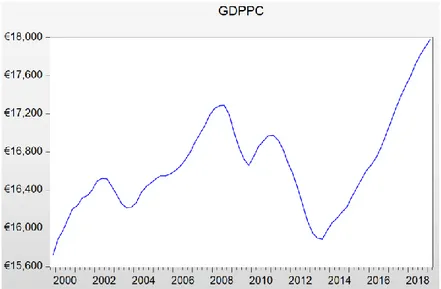
Figure 2: The evolution of GDPPC, Q4 1999 – Q1 2019

Source: INE – Statistics Portugal

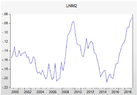
The first measure of financial development is the ratio of bank liquid deposit liabilities, measured by the money stock M2, excluding currency in circulation, to nominal GDP (LNM2) [King and Levine (1993a, 1993b), Demetriades and Hussein (1996), Arestis

23

and Demetriades (1997) and Xu (2000)]. The intuition behind this financial development indicator is to assess whether an increase in the size of banks improves its capacity to provide financial services [Goldsmith (1969) as cited in King and Levine (1993a)]. An increase in deposit liabilities provide more means for banks to finance the economy, but it does not guarantee that they will be doing it. Deposit liabilities are banks’ most important and cheapest funding source, but not the only one possible, as banks may also fund themselves by borrowing from the interbank lending market and the central bank, or by issuing debt securities. Figure 2 shows the evolution of LNM2 throughout the sample period.

Figure 3: The evolution of LNM2, Q4 1999 – Q1 2019

Source: BPstat – Banco de Portugal and INE – Statistics Portugal

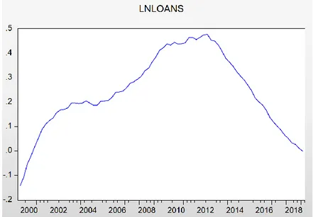
The second financial development indicator is the ratio of bank loans to nominal GDP (LNLOANS), partially derived from King and Levine (1993a, 1993b), Demetriades and Hussein (1996) and Arestis and Demetriades (1997). It comprises loans from other monetary financial institutions1 to households, non-financial corporations, non-monetary financial corporations, and general government, due to the importance of the public sector in the

24

Portuguese economy. According to the McKinnon/Shaw inside money model, as cited in Demetriades and Hussein (1996), the supply of credit to the private sector is ultimately responsible for the quantity and quality of investment and, in turn, for economic growth. Portuguese banks’ business model is focused on lending: loans to customers (net) reached 70% of total assets of the Portuguese banking sector in 2008. Thus, by measuring a crucial part of Portuguese banks’ financial intermediation output, this indicator is expected to exert more direct causal influence on economic growth and provide additional insight into the finance and growth nexus. Figure 3 shows the evolution of LNLOANS throughout the sample period.

Figure 4: The evolution of LNLOANS, Q4 1999 – Q1 2019

Source: Statistical Data Warehouse – European Central Bank and INE – Statistics Portugal All series are on a quarterly basis and span from Q4 1999 to Q1 2019, the quarters after the Euro adoption from which we can obtain consistent data. The introduction of the Euro was a crucial economic and financial development that changed the way banks and other economic agents behaved. It eliminated the exchange rate risk against those member states facilitating the obtention of liquidity by banks and, by sharing the same currency with

25

other rich countries, it also contributed to a reduction of real interest rates and banking spreads for households and corporations in Portugal.

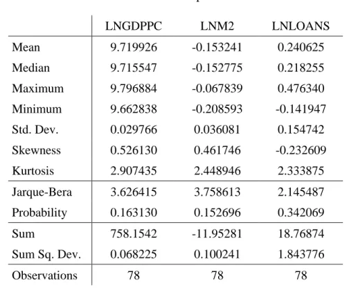
Each indicator was built using arithmetic averages to solve the problem of dividing stocks (money stock, loans, and population) by flows (GDP), and vice-versa. An increase in each of the ratios should be interpreted as an increase in financial development (financial deepening). Also, to ease the interpretation of the results, we transformed all these variables into natural logarithms. All data was sourced from INE – Statistics Portugal (GDP and resident population), BPstat – Banco de Portugal (money stock M2, excluding currency) and the Statistical Data Warehouse of the European Central Bank (bank loans). Data descriptive statistics are presented in Table A1.

5.RESULTS

5.1.M2 AS A FINANCIAL DEVELOPMENT INDICATOR

The first set of tests were performed to assess the relationship between LNGDPPC and LNM2 as a financial development indicator.

Table 1: Results of the Johansen cointegration test with LNGDPPC and LNM2

Null

hypothesis Trace statistic

5% critical value Maximum eigenvalue statistic 5% critical value r=0 18.90183 15.49471 15.19740 14.26460 r≤1 3.704431 3.841466 3.704431 3.841466 r is the number of cointegrating vectors

The results of the Johansen cointegration test (Table 1), using both trace and maximum eigenvalue statistics, allow us to reject the null hypothesis of no cointegration equations between LNM2 and LNGDPPC at the 5% level. Further, using both statistics, the

26

second null hypothesis of at most one cointegration equation among the variables could not be rejected. Thus, there is evidence of cointegration between LNM2 and LNGDPPC.

The existence of cointegration between LNM2 and LNGDPPC corresponds to stating that financial development and economic growth have a long-run relationship. It implies that both series are related and that if there are shocks that affect their movement in the short-run, both series would still converge in the long-run.

Due to these results, a Vector Error Correction Model (VECM) was estimated to account for both the short-run and long-run relationship among the variables:

ΔLNGDPPCt = α + ∑ 𝑘 − 1 𝑖 = 1βiΔLNGDPPCt-i + ∑ 𝑘 − 1 𝑗 = 1ΦjΔLNM2t-j + λ1ECTt-1 + µ1t (9) ΔLNM2t = σ + ∑ 𝑘 − 1 𝑖 = 1βiΔLNGDPPCt-i + ∑ 𝑘 − 1 𝑗 = 1ΦjΔLNM2t-j + λ2ECTt-1 + µ2t (10)

Table 2: Causality tests results of the VECM

Null hypothesis:

LNM2 does not cause LNGDPPC ECT t-statistic λ1=0 Granger/Wald Φ1=…=Φ4=0 Pairwise Granger causality test Wald λ1=Φ1=…=Φ4=0 0.24 4.54 1.01 4.71 Null hypothesis:

LNGDPPC does not cause LNM2 ECT t-statistic λ2=0 Granger/Wald β1=…=β4=0 Pairwise Granger causality test Wald λ2=β1=…=β4=0 3.62(2) _15.22(2) _7.92(2) _49.95(2)

Statistics are presented in absolute value.

(1) _{Rejected at the 5% level.} (2) _{Rejected at the 1% level.}

The causality tests performed in the VECM system (Table 2) show that, both the significance of the error correction term (λ2) at the 1% level when LNM2 is the dependent

27

variable, and the no significance of the error correction term (λ1) when LNGDPPC is the

dependent variable are evidence of long-run unidirectional causality from LNGDPPC to LNM2.

Concerning the short-run relationship, no lagged explanatory variable is individually significant at the 5% level. LNM2(-1) is significant but only at the 10% level, when LNGDPPC is the dependent variable, and LNGDPPC(-1) is also significant at the 10% level when LNM2 is the dependent variable.

In both the Granger/Wald causality tests on lagged explanatory variables and the Pairwise Granger causality tests, I rejected the null hypothesis of no Granger causality from LNGDPPC to LNM2 at the 1% level.

The lagged explanatory variables and the error correction term were also jointly tested (Wald), and I rejected the null hypothesis of no significance at the 1% level, which implies strong unidirectional causal effects from LNGDPPC to LNM2.

Hence, the t-statistics of the error correction term, as well as the chi-squared statistics from Granger/Wald and Wald coefficient tests, and the F-statistics from the Pairwise Granger causality tests show strong evidence of both short-run and long-run unidirectional causality from LNGDPPC to LNM2.

28

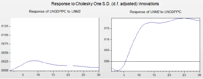
Figure 5: Impulse response functions results for the VECM

The results of the IRF for this system (Figure 4) describe the impulses and responses of both variables when they serve as independent and dependent variables, respectively, in the system, to a one-time standard deviation shock to the corresponding independent variable. The IRF results show that a positive shock to LNGDPPC has a significant positive permanent effect on LNM2 in the long-run. One standard deviation shock to LNGDPPC leads to a permanent increase in LNM2 of 0,019%, and one standard deviation shock to LNM2 leads to a permanent increase in LNGDPPC of less than 0,001%. This difference corroborates the results from Johansen’s cointegration and Granger causality tests.

It is also important to highlight that, in the short-run, both the effect and the sign of the causal relationship from LNGDPPC to LNM2 are different from the long-run, as the response of LNM2 to one standard deviation shock to LNGDPPC is negative in the short-run, peaking at -0,0042%, and positive in the long-run.

In conclusion, using LNM2 as a financial development indicator, an increase in financial development does not have a significant impact on economic growth, both in the short-run and in the long-run, but economic growth has a significant effect on financial

29

development, in line with Demetriades and Hussein (1996). That effect is negative in the short-run and positive in the long-run.

5.2.LOANS AS A FINANCIAL DEVELOPMENT INDICATOR

The second set of tests were performed to assess the relationship between LNGDPPC and LNLOANS as a financial development indicator.

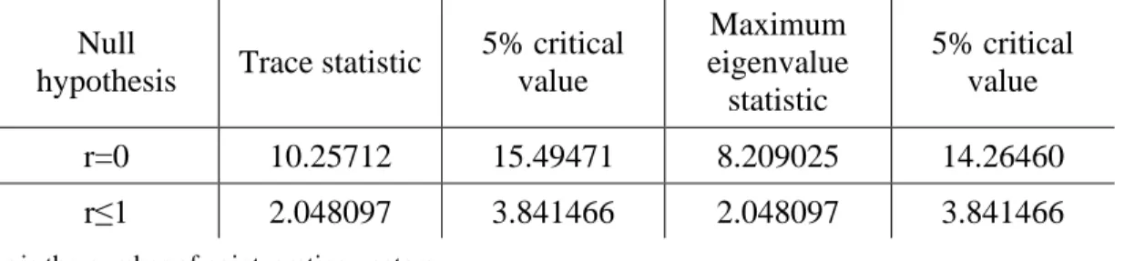
Table 3: Results of the Johansen cointegration test with LNGDPPC and LNLOANS

Null

hypothesis Trace statistic

5% critical value Maximum eigenvalue statistic 5% critical value r=0 10.25712 15.49471 8.209025 14.26460 r≤1 2.048097 3.841466 2.048097 3.841466 r is the number of cointegrating vectors.

The results of the Johansen cointegration test (Table 3), using both trace and maximum eigenvalue statistics, do not allow us to reject the null hypothesis of no cointegration equations between LNLOANS and LNGDPPC at the 5% level. Hence, there is no evidence of cointegration among the variables. These results do not corroborate the findings of previous studies that used financial development proxies related to lending, namely Demetriades and Hussein (1996).

Due to these results, we estimated a VAR model to analyse only the short-run relationship among the variables:

LNGDPPCt = α + ∑ 𝑘 − 1 𝑖 = 1βiLNGDPPCt-i + ∑ 𝑘 − 1 𝑗 = 1ΦjLNLOANSt-j + µ1t (11) LNLOANSt = σ + ∑ 𝑘 − 1 𝑖 = 1βiLNGDPPCt-i + ∑ 𝑘 − 1 𝑗 = 1ΦjLNLOANSt-j + µ2t (12)

30

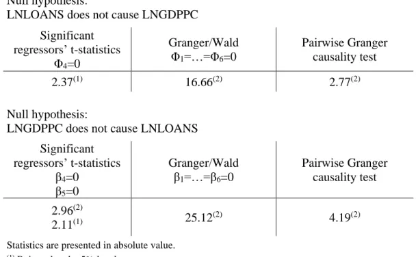
Table 4: Causality tests results of the VAR

Null hypothesis:

LNLOANS does not cause LNGDPPC Significant regressors’ t-statistics Φ4=0 Granger/Wald Φ1=…=Φ6=0 Pairwise Granger causality test 2.37(1) _16.66(2) _2.77(2) Null hypothesis:

LNGDPPC does not cause LNLOANS Significant regressors’ t-statistics β4=0 β5=0 Granger/Wald β1=…=β6=0 Pairwise Granger causality test 2.96(2) 2.11(1) 25.12 (2) _4.19(2)

Statistics are presented in absolute value.

(1) _{Rejected at the 5% level.} (2) _{Rejected at the 1% level.}

The causality tests performed in the VAR system (Table 4) show that, concerning the significance of the regressors, when LNGDPPC is the dependent variable, LNLOANS(-4) is significant at the 5% level. LNGDPPC(-5) and LNGDPPC(-6) are also significant at the 5% level of less when LNLOANS is the dependent variable.

In both the Granger/Wald causality tests on lagged explanatory variables and the Pairwise Granger causality tests, the null hypothesis of no Granger causality from LNLOANS to LNGDPPC, and vice-versa, was rejected at the 5% level or less.

Hence, the t-statistics of the regressors, as well as the F-statistics from Granger/Wald tests and the chi-squared statistics from the Pairwise Granger causality tests indicate short-run bi-directional causality between financial development and economic growth.

31

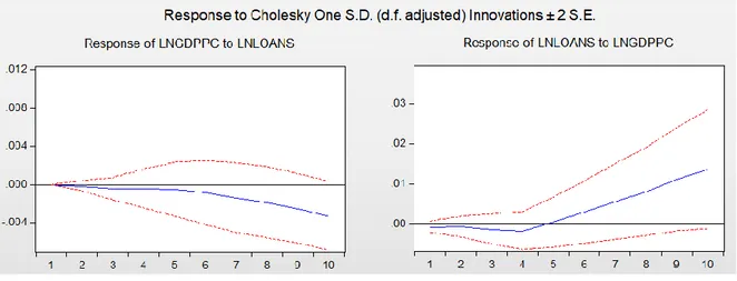
Figure 6: Impulse response functions results for the VAR

The results of the IRF for this system (Figure 5) show that one standard deviation shock to LNLOANS generates a negative but almost unnoticeable response from LNGDPPC in the first four quarters. However, from the 5th _{quarter onwards, the response of LNGDPPC}

gradually declines and becomes systematically more negative after each quarter. The response of LNLOANS to a shock in LNGDPC is also negative and muted in the first four quarters but sharply increases to positive values in the 5th quarter, showing an increasing tendency in each of the next quarters.

Thus, the IRF results allow us to conclude that, after the 5th _{quarter, the bi-directional}

causality among the variables is shown to be divergent, with opposite signs and different magnitudes, as a shock to LNGDPPC generates a positive and stronger response of LNLOANS, whereas a shock to LNLOANS induces a negative and less stronger response of LNGDPPC.

In conclusion, in the short-run, using LNLOANS as a financial development indicator, an increase in finance development has a negative effect on economic growth, but economic growth has a positive effect on financial development, in line with Demetriades and Hussein (1996). However, concerning the long-run, the results of the Johansen

32

cointegration test found no evidence of cointegration among the variables, that is, LNLOANS and LNGDPPC do not have a long-run relationship. This result might be due to the opposite effect that the variables have on each other.

5.3.DIAGNOSTICS

A set of diagnostic tests were performed on the residuals and on the stability of both models to assess the robustness and reliability of the study, namely: autocorrelation LM test, normality test, heteroscedasticity test, and the Roots of Characteristic Polynomial (only in the VAR model).

The results of the residual tests are presented in Tables A5-A7 and A9-A11 of the Appendix. In the autocorrelation LM test, we failed to reject the null hypothesis of no serial correlation in the residuals in both models at the 5% level. The normality test shows that the residuals are also normally distributed in both models. In the heteroscedasticity test, we failed to reject the null hypothesis of no heteroscedasticity in both models at the 5% level.

Concerning stability diagnostics, in the Roots of the Characteristic Polynomial, in the VAR model, all roots have modulus less than one and lie inside the unit circle, which implies that the model is stable, and its results are valid. The results are presented in Table A12 of the Appendix.

5.4.DISCUSSION AND LIMITATIONS

The most important result of this study is that an increase in financial development does not exert a positive effect on economic growth in Portugal. Instead, this empirical assessment offers compelling support to the idea of reverse causality among the variables.

The result of M2 as a financial development indicator supports the view championed by Robinson (1952), as cited in King and Levine (1993a), and Lucas (1988) that finance

33

development simply evolves to meet the growing demand of services by the real sector and does not seem to have a meaningful effect on economic growth. Also, it supports the idea detailed by King and Levine (1993a) that the pure size of the financial system may not be closely related to its capacity to provide financial services such as risk management and information processing, which are key aspects in the dealings of financial intermediation.

Concerning LNLOANS as a financial development indicator, the result is slightly different but much more insightful. All causality tests performed, as well as IRF results, indicate the existence of short-run bi-directional causality between LNLOANS and LNGDPPC, but in the case of causality from LNLOANS to LNGDPPC, the relationship is negative. This result shows that banks’ lending does not significantly boost output both in the short-run and in the long-run. Rather, it seems to have a negative impact on real per capita GDP. This impact should be due to the increase in the indebtedness of the Portuguese economy in the period of this study, which resulted in a severe recession. In previous studies for Portugal, Demetriades and Hussein (1996) only analyse the years before the adoption of the Euro but conclude that financial development does not cause economic growth in Portugal.

In fact, after the adoption of the Euro, the ease with which Portuguese banks obtained liquidity through foreign financial institutions, which resulted in a loan-to-deposit ratio that peaked at 160.5% in March 2008 [Banco de Portugal (2019b)], did not translate into a significant increase in output. Instead, an important part of those resources was channelled to the acquisition of imports (Portugal had current account deficits of over 7% of GDP between 2000 and 2010) and for investment in non-tradable sectors. Thus, the excess indebtedness of the economy caused by this capital flow bonanza resulted in a bailout by the

34

Troika2, with the implementation of the Economic and Financial Assistance Program between 2011 and 2014, which induced a severe recession in the Portuguese economy.

An important limitation of this study is related to the availability of data on financial intermediation output. The LNLOANS variable using in this study, or any other lending variable available which could have been used, is collected from the other monetary financial institutions’ actual aggregate balance-sheet. However, banking practices over the past 10 to 15 years have generated a significant difference between loans originated by banks and loans which are still on their balance-sheets.

On the one hand, especially until the global financial crisis, banks regularly carried out securitization3 _{operations, which allowed to finance the origination of new loans while at}

the same time some were derecognized from the banks’ lending portfolio. On the other hand, since the economic crisis that ensued the Economic and Financial Adjustment Program, banks registered a significant increase in non-performing loans on their balance-sheets, which peaked at 50.5 billion euros in June 2016 [Banco de Portugal (2019a)]. Ever since, banks have sold a significant part of these loans, together with other performing loans, to increase investors’ appetite and improve their asset quality, and profitability. As a result, non-performing loans decreased to 24.4 billion euros in March 2019 [Banco de Portugal (2019a)].

In conclusion, there is a large unaccounted amount of loans originated by banks, still being paid or even managed by banks, not included in lending statistics that contribute to a devaluation of the banks’ financial intermediation output in this study.

2 _{Group formed by the European Commission, the European Central Bank and International Monetary Fund.} 3 _{Securitization is the process of pooling together various types of debt instruments (assets) such as mortgage}

35

6.CONCLUSIONS

This dissertation analysed the impact of financial development provided by banks in economic growth in Portugal, using two measures of financial development: the ratios of bank liquid deposit liabilities (LNM2) and bank loans (LNLOANS), to nominal GDP.

We found that an increase in financial development does not have a positive and significant effect on economic growth. Instead, this dissertation offers compelling support to the idea of reverse causality among the variables, with economic growth exerting a positive effect on financial development and not the opposite, in line with Demetriades and Hussein (1996).

Using M2 as a financial development indicator, the cointegration tests reveal the existence of a long-run relationship between this variable and real per capita GDP. However, causality tests show that economic growth is the leading variable in this relationship, with causality running from real per capita GDP to M2.

More interesting are the results using LNLOANS as a financial development indicator, as this variable is the one which is expected to exert a more direct causal effect on economic growth, according to the McKinnon/Shaw inside money model, as cited in Demetriades and Hussein (1996), as lending to the private sector is responsible for the quantity and quality of investment and, in turn, for economic growth. Causality tests show the existence of bi-directional short-run causality among the variables. However, in the case of causality from bank loans to real per capita GDP, the relationship is negative. These results are very relevant and show that banks’ lending did not increase economic growth both in the short-run and in the long-run in Portugal since the adoption of the Euro. Instead, lending had a negative impact on economic growth. However, it is important to mention that the results

36

of this study are conditioned by the period of the Troika and the Economic and Financial Adjustment Program, which induced a severe recession in the Portuguese economy.

In conclusion, this study supports the view championed by Robinson (1952), as cited in King and Levine (1993a), and Lucas (1988), that finance development only evolves to meet the growing demand for services by the real sector and does not have a significant effect on economic growth.

For future research to provide more insights on the finance-growth nexus, statistical sources need to improve the quality of their data, finding ways to account for the outstanding amount of loans originated by banks in the economy, and not only the loans registered on banks’ balance-sheets.

REFERENCES

Arcand, J-L., Berkes, E. & Panizza, U. (2012). Too Much Finance? IMF Working Paper No. 12/161.

Arellano, M. & Bover, O. (1995). Another look at the instrumental-variable estimation of error-components models. Journal of Econometrics 68, 29-52.

Arestis, P. & Demetriades, P. (1997). Financial development and economic growth: Assessing the evidence. Economic Journal 107, 783-799.

Banco de Portugal (2019a). Portuguese Banking System: latest developments - 1st _quarter

2019 [Online], 19 June 2019. Lisbon: Banco de Portugal. Available in:

https://www.bportugal.pt/sites/default/files/anexos/pdf-boletim/overviewportuguesebankingsystem_2019q1_en.pdf [Access in: 2019/09/05].

Banco de Portugal (2019b). Portuguese banking sector indicators [Database], October 2019.

37

https://www.bportugal.pt/EstatisticasWeb/(S(xteekzymyuwpv055dxdq1buu))/DEFA ULT.ASPX?Lang=en-GB

Bagehot, W. (1873). Lombard Street: A Description of the Money Market, 3rd _{Ed. London:}

Henry S. King & Co..

Beck, T. (2012). Finance and growth – lessons from the literature and the recent crisis. Prepared for the LSE Growth Commission, July 2012.

Beck, T. & Levine R. (2002). Industry growth and capital allocation: Does have a market- or bank-based system matter? Journal of Finance 60, 137-177.

Beck, T., Levine, R. & Loayza, N. (2000). Finance and the sources of growth. Journal of

Financial Economics 58, 261-300.

Britannica (2019). Securitization | Definition & Facts [Online]. Available in:

https://www.britannica.com/topic/securitization [Access in: 2019/09/15].

Brown, J., Martinsson, G. & Petersen, B. (2013). Law, stock markets, and innovation.

Journal of Finance 68 (4), 1517-1549.

Chakraborty, I., Goldstein, I. & MacKinlay, A. (2014). Do Asset Price Booms have Negative Real Effects? Wharton School working paper.

Demetriades. P. & Hussein, K. (1996). Does financial development cause economic growth? Time-series evidence from 16 countries. Journal of Development Economics 51, 387-411.

Demirgüç-Kunt, A., Feyen, E. & Levine R. (2012). The evolving importance of banks and securities markets. NBER working paper 18004.

Demirgüç-Kunt A & Huizinga H. (2010). Bank activity and funding strategies: The impact on risk and return. Journal of Financial Economics 98, 626-650.

38

Demirgüç-Kunt, A. & Levine, R. (2001). Financial Structures and Economic Growth: A

Cross-Country Comparison of Banks, Markets and Development. Cambridge, MA:

MIT Press.

Demirgüç-Kunt, A. & Maksimovic, V. (2002). Funding growth in bank-based and market-based financial systems: Evidence from firm level data. Journal of Financial Economic 65, 337-363.

Engle, R.F. & Granger, C.W.J. (1987). Co-integration and error correction: representation, estimation and testing. Econometrica 55, 1057-1072.

European Parliament and the Council of the European Union (2013). Regulation (EU) No

575/2013 of the European Parliament and of the Council of 26 June 2013 on prudential

requirements for credit institutions and investment firms and amending Regulation

(EU) No 648/2012 Text with EEA relevance [Online]. Available in:

https://eur-lex.europa.eu/legal-content/EN/TXT/?uri=CELEX:32013R0575 [Access in:

2019/09/05].

European Parliament and the Council of the European Union (2014). Directive 2014/59/EU

of the European Parliament and of the Council of 15 May 2014 establishing a

framework for the recovery and resolution of credit institutions and investment firms

and amending Council Directive 82/891/EEC, and Directives 2001/24/EC,

2002/47/EC, 2004/25/EC, 2005/56/EC, 2007/36/EC, 2011/35/EU, 2012/30/EU and

2013/36/EU, and Regulations (EU) No 1093/2010 and (EU) No 648/2012, of the

European Parliament and of the Council Text with EEA relevance [Online]. Available

in: https://eur-lex.europa.eu/legal-content/EN/TXT/?uri=celex:32014L0059 [Access