Network distributed 3D video quality monitoring system

Departamento

de Engenharia Electrotécnica

Network Distributed 3D Video Quality

Monitoring System

Trabalho de Projeto apresentado para a obtenção do grau de Mestre em

Automação e Comunicações em Sistemas de Energia

Autor

Nuno Alexandre Bettencourt Martins

Orientador

Doutor Fernando José Pimentel Lopes

Instituto Superior de Engenharia de Coimbra

I would like to declare my sincere acknowledgements to everyone that helped me during this research work.

I would like to begin by expressing my gratitude to my supervisor, Professor Fernando Lopes whose guidance and availability were essential for this project completion.

I would like to thank Professor Lu´ıs Cruz and the 3DVQM - 3D Video Quality Monitor Project (IT/LA/P01131/2011) the opportunity to work as a researcher in this project and for the guidance, support, time to discuss technical aspects and add new ideas during the work development. I also would like to thank Instituto de Telecomunica¸c˜oes for the laboratory facilities and conditions to accomplish this work. Thanks to my research lab colleagues Guilherme, Tha´ısa and specially Pedro for the help on completing the project demonstration.

Finally, a special thanks to my parents, Rosa and Armindo, my sister C´atia, my girlfriend Guida and my great friend Alex. To them I owe all that I have become. Thank you for being there.

This project description presents a research and development work whose primary goal was the design and implementation of an Internet Protocol (IP) network distributed video quality assessment tool. Even though the system was designed to monitor H.264 three-dimensional (3D) stereo video quality it is also applicable to different formats of 3D video (such as texture plus depth) and can use different video quality assessment models making it easily customizable and adaptable to varying conditions and transmission scenarios.

The system uses packet level data collection done by a set of network probes located at convenient network points, that carry out packet monitoring, inspection and analysis to obtain information about 3D video packets passing through the probe’s locations. The information gathered is sent to a central server for further processing including 3D video quality estimation based on packet level information.

Firstly an overview of current 3D video standards, their evolution and features is presented, strongly focused on H.264/AVC and HEVC. Then follows a description of video quality assessment metrics, describing in more detail the quality estimator used in the work. Video transport methods over the Internet Protocol are also explained in detail as thorough knowledge of video packetization schemes is important to understand the information retrieval and parsing performed at the front stage of the system, the probes.

After those introductory themes are addressed, a general system architecture is shown, explaining all its components and how they interact with each other. The devel-opment steps of each of the components are then thoroughly described.

In addition to the main project, a 3D video streamer was created to be used in the implementation tests of the system. This streamer was purposely built for the present work as currently available free-domain streamers do not support 3D video streaming.

The overall result is a system that can be deployed in any IP network and is flexible enough to help in future video quality assessment research, since it can be used as a testing platform to validate any proposed new quality metrics, serve as a network monitoring tool for video transmission or help to understand the impact that some network characteristics may have on video quality.

Este relat´orio de projeto apresenta o trabalho de pesquisa e desenvolvimento no qual o principal objetivo foi o desenvolvimento e implementa¸c˜ao de um sistema de determ-ina¸c˜ao da qualidade de v´ıdeo em redes IP distribu´ıdas. Apesar de ser destinado `a mon-itoriza¸c˜ao da qualidade de v´ıdeo 3D codificado usando a especifica¸c˜ao H.264 para v´ıdeo estereosc´opico, ´e tamb´em poss´ıvel o seu uso para testar diversos outros formatos de v´ıdeo 3D (tais como textura mais profundidade) assim como diferentes modelos de de-termina¸c˜ao de qualidade de v´ıdeo, tornado-o numa solu¸c˜ao facilmente personaliz´avel e adaptada a diversas condi¸c˜oes e cen´arios de transmiss˜ao.

O sistema utiliza informa¸c˜oes recolhidas por um conjunto de sondas, conveniente-mente distribu´ıdas por diversos pontos da rede, respons´aveis por monitorizar, inspecionar e analisar pacotes de rede de maneira a obter informa¸c˜oes acerca de v´ıdeo 3D que esteja a passar pelas localiza¸c˜oes das sondas. As informa¸c˜oes recolhidas s˜ao enviadas para um servidor central para serem processadas de modo a estimar a qualidade de v´ıdeo 3D.

Em primeiro lugar ´e apresentado um resumo da evolu¸c˜ao e caracter´ısticas dos stand-ards de v´ıdeo 3D, descrevendo em mais detalhe o H.264/AVC e o HEVC. Segue-se depois a descri¸c˜ao de m´etricas para a determina¸c˜ao da qualidade de v´ıdeo, explicando a m´etrica utilizada para validar o trabalho desenvolvido. Os m´etodos de transporte de v´ıdeo sobre redes IP s˜ao tamb´em descritos, para que se possa perceber com o ´e efetuada a an´alise dos pacotes de rede capturados e como deles s˜ao determinadas as informa¸c˜oes necess´arias ao n´ıvel das sondas do sistema.

Ap´os a apresenta¸c˜ao dos temas que definem o enquadramento do trabalho, segue-se uma descri¸c˜ao da arquitetura geral do sistema, detalhando conceptualmente todos os seus componentes e mostrando a forma como estes interagem para formar um todo funcional. Apresenta-se seguidamente uma descri¸c˜ao pormenorizada dos v´arios passos que foram implementados no desenvolvimento de cada um dos componentes do sistema global.

Foi criado um emissor de v´ıdeo 3D como complemento ao projeto principal, para que fosse poss´ıvel testar as implementa¸c˜oes realizadas uma vez que n˜ao existe at´e ao momento software livre capaz emitir v´ıdeo por uma rede IP.

O resultado ´e um sistema capaz de ser instalado em qualquer rede IP, flex´ıvel o sufi-ciente para ajudar em futuros avan¸cos no desenvolvimento de m´etricas de determina¸c˜ao da qualidade de v´ıdeo, uma vez que pode ser usado como plataforma de testes para Network Distributed 3D Video Quality Monitoring System vii

Contents ix

List of Figures xiii

List of Tables xv

List of Code Examples xvii

List of Abbreviations xxi

1 Introduction 1

1.1 Context and Motivation . . . 1

1.2 Objectives . . . 2 1.3 Outline . . . 3 2 Video Coding 5 2.1 Video Standards . . . 5 2.1.1 H.264/AVC . . . 6 2.1.2 HEVC . . . 10 2.2 3D Video Coding . . . 12

2.2.1 H264/AVC Multi-View video Coding . . . 12

3 Video Transport 15 3.1 Video Packetization . . . 15

3.1.1 Internet Protocol . . . 15

3.1.2 User Datagram Protocol . . . 15

3.1.3 Real-time Transport Protocol . . . 16

3.1.4 MPEG 2 Transport Stream . . . 16

3.1.5 MPEG2-TS transport methods . . . 22

3.2 3D MPEG2-TS encapsulation . . . 22

4 3D Video Qualiy Models 25 4.1 NR Quality Models . . . 26

4.1.1 Proposed NR model . . . 27 Network Distributed 3D Video Quality Monitoring System ix

4.1.2 Quality model overview . . . 28

5 Distributed Architecture 31 5.1 Proposed Architecture . . . 31

5.2 Probe . . . 33

5.2.1 Packet Monitoring . . . 34

5.2.2 Finding Video PIDs . . . 37

5.2.3 Packet Parser . . . 38

5.2.4 Information constraint . . . 40

5.2.5 Report to Server . . . 40

5.2.6 Usage and Versions . . . 41

5.3 Server . . . 41

5.3.1 Video Quality Assessment calculation . . . 42

5.4 Graphical User Interface . . . 43

5.4.1 Connection and Probe Status . . . 44

5.4.2 Capture Configuration . . . 45

5.4.3 Video Quality Assessment Graphs . . . 45

5.5 Database . . . 47

5.5.1 Table description . . . 47

5.6 Future HEVC implementation . . . 50

6 Functional tests 53 6.1 MPEG2-TS 3D Video Streamer . . . 53

6.1.1 Packet loss using the Gilbert-Elliot model . . . 55

6.2 Test Environment . . . 57

6.3 Reliability tests . . . 58

6.4 NR Video Quality Model Tests . . . 59

6.4.1 NR Model Parameters . . . 59

6.4.2 NR Model Tests . . . 59

7 Conclusions and future work 65 7.1 Conclusions . . . 65

7.2 Future work . . . 66

Bibliography 67

Appendix 71

A NAL Unit Types 71

B Function responsible for quality metric calculation 73

D Graphical User Interface 79

E Function implementing the Gilbert-Elliot model 81

F Pictures ilustrating video degradation 83

F.1 Dog sequence . . . 83

F.2 Balloons sequence . . . 87

F.3 Bullinger sequence . . . 90

F.4 ESTG Bus Stop sequence . . . 93

1.1 3D Video Quality Monitoring scenario . . . 1

2.1 H.264 Layer Structure (adapted from [1]) . . . 6

2.2 GOP frame reference relationship . . . 8

2.3 4x4 prediction modes [2] . . . 8

2.4 NALU header structure . . . 9

2.5 CTB partitioning and corresponding quadtree (adapted from [3]) . . . 11

2.6 HEVC prediction modes [4] . . . 11

2.7 Picture prediction relation in MVC (adapted from [5]) . . . 13

2.8 MVC NALU header structure . . . 14

3.1 PES packet structure . . . 18

3.2 TS packet structure . . . 21

3.3 Comparison between transport methods . . . 22

3.4 Illustration of MVC bitstream encapsulation into TS . . . 23

4.1 SSIM computation [6] . . . 28

4.2 Delta SSIM vs frame size loss for one particular test Dataset[6] . . . 29

4.3 Packet layer model structure [6] . . . 29

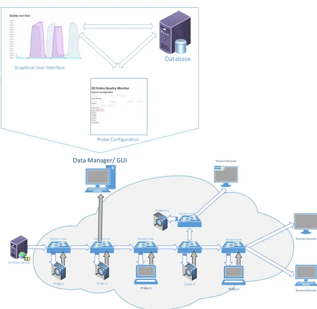
5.1 Proposed system architecture overview: white arrows - video/network traffic; grey arrows - Probe report data . . . 32

5.2 Port Mirroring illustration . . . 33

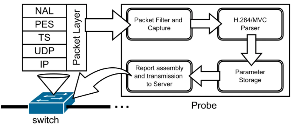
5.3 Probe high level block diagram . . . 34

5.4 Probe operation flowchart . . . 35

5.5 Parse frames program flowchart . . . 39

5.6 Server functional blocks . . . 42

5.7 Interface: Probe Status and Configuration . . . 44

5.8 Interface: Instant quality . . . 46

5.9 Interface: Quality progress for a single Probe . . . 46

5.10 Interface: Table with general information from the captured video . . . . 47

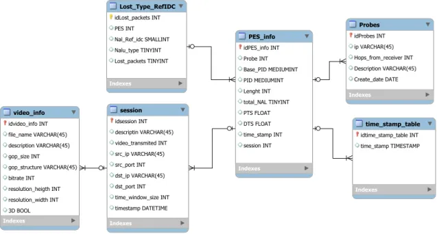
5.11 Entity Relationship Diagram of the system database . . . 48

5.12 HEVC NALU header fields . . . 51 Network Distributed 3D Video Quality Monitoring System xiii

6.1 Auxiliary file generation for 3D video Streamer . . . 54

6.2 3D video Streamer block diagram . . . 55

6.3 Gilbert-Elliot model representation . . . 56

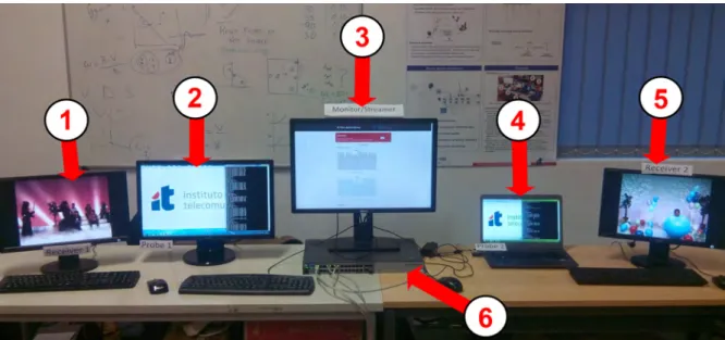
6.4 Experimental setup . . . 58

6.5 dSSIM in function of packet losses . . . 60

6.6 Video sequences used for metric evaluation . . . 61

6.7 Calculated dSSIM values by Probe report . . . 62

6.8 Base and secondary views dSSIM comparison . . . 63

6.9 dSSIM in function of UDP packet loss percentage . . . 63

D.1 Graphical User Interface Layout . . . 80

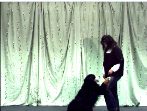
F.1 Still image from DOG sequence, for 0.1% UDP packet losses . . . 83

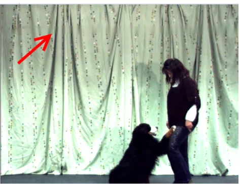
F.2 Still image from DOG sequence, for 0.5% UDP packet losses . . . 84

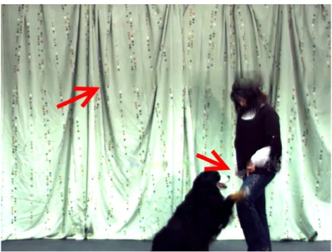
F.3 Still image from DOG sequence, for 1% UDP packet losses . . . 84

F.4 Still image from DOG sequence, for 2% UDP packet losses . . . 85

F.5 Still image from DOG sequence, for 4% UDP packet losses . . . 85

F.6 Still image from DOG sequence, for 8% UDP packet losses . . . 86

F.7 Still image from Balloons sequence, for 0.1% UDP packet losses . . . 87

F.8 Still image from Balloons sequence, for 0.5% UDP packet losses . . . 87

F.9 Still image from Balloons sequence, for 1% UDP packet losses . . . 88

F.10 Still image from Balloons sequence, for 2% UDP packet losses . . . 88

F.11 Still image from Balloons sequence, for 4% UDP packet losses . . . 89

F.12 Still image from Balloons sequence, for 8% UDP packet losses . . . 89

F.13 Still image from Bullinger sequence, for 0.1% UDP packet losses . . . 90

F.14 Still image from Bullinger sequence, for 0.5% UDP packet losses . . . 90

F.15 Still image from Bullinger sequence, for 1% UDP packet losses . . . 91

F.16 Still image from Bullinger sequence, for 2% UDP packet losses . . . 91

F.17 Still image from Bullinger sequence, for 4% UDP packet losses . . . 91

F.18 Still image from Bullinger sequence, for 8% UDP packet losses . . . 92

F.19 Still image from ESTG Bus Stop sequence, for 0.1% UDP packet losses . 93 F.20 Still image from ESTG Bus Stop sequence, for 0.5% UDP packet losses . 93 F.21 Still image from ESTG Bus Stop sequence, for 1% UDP packet losses . . 94

F.22 Still image from ESTG Bus Stop sequence, for 2% UDP packet losses . . 94

F.23 Still image from ESTG Bus Stop sequence, for 4% UDP packet losses . . 94

6.1 Video sequence characteristics . . . 62 A.1 NAL unit type codes, syntax element categories, and NAL unit type classes 72 C.1 Curve fitting coefficients for P-frames . . . 78 C.2 Curve fitting coefficients for B-frames . . . 78

5.1 Packet structure example, missing definition of MPEG-TS and PES for

simplicity . . . 36

5.2 Parsed information structure . . . 38

5.3 Example of Probe data variables access . . . 42

5.4 Example of a Database query . . . 50

B.1 Example of VQA metric calculation . . . 73

E.1 Example of Gilbert-Elliot model implementation . . . 81

2D two-dimensional. 2, 11, 31, 34

3D three-dimensional. v, 1–3, 11, 16, 22, 24, 31, 33 AU Access Unit. 8

AVS Audio Video Standard. 5

CABAC Context-adaptive binary arithmetic coding. 7 CAVLC Context-adaptive variable-length coding. 7 CB Coding Block. 9

CSV Classical Stereo Video. 11 CTB Coding Tree Block. xi, 9, 10 CTU Coding Tree Units. 9

CU Coding Unit. 9, 10

DCT Discrete Cosine Transform. 8

DPCM Differential Pulse Code Modulation. 5 ES Elementary Streams. 16, 22

GOP Group of Pictures. 24, 29 GUI Graphical User Interface. 3, 29 HD High Definition. 5

HEVC High Efficiency Video Coding. 3, 9 IP Internet Protocol. v, 2, 3, 15, 20, 29–31, 33 IPTV television broadcast over the internet. 1, 6

JCT-VC Joint Collaborative Team on Video Coding. 9 JVT Joint Video Team. 6

LDV Layered Depth Video. 11

MPEG Moving Pictures Experts Group. 6, 9

MPEG2-TS MPEG 2 Transport Stream. 16, 20, 25, 31, 34 MRS Mixed Resolution Stero. 11

MSE Mean Square Error. 24

MVC Multi-View video Coding. 11, 12, 22 MVD Multi-View Video plus Depth. 11, 56 MVV Multi-View Video. 11

NAL Network Abstraction Layer. 8 NALU NAL Unit. 8, 11, 12, 16 P2P Peer-to-Peer. 1

PB Prediction Block. 10

PES Packetized Elementary Streams. 16, 18–20, 22, 35 PID Packet Identifier. 19, 20, 22, 35

PPS Picture Parameter Sets. 8

PSNR Peak signal-to-noise ratio. 6, 24 PU Prediction Unit. 10

QoE Quality of Experience. 1 QP Quantitization Parameter. 8, 24 RBSP raw byte sequence payload. 8 RDO Rate distortion Optimization. 10

RTP Real-time Transport Protocol. 15, 16, 20 SD Standard Definition. 5

SPS Sequence Parameter Sets. 8 SSIM Structural Similarity. 24, 25

TS Transport Stream. 18–20, 22, 33, 34, 38 TU Transform Unit. 10

UDP User Datagram Protocol. 15, 20, 33 UHD Ultra Hight Definition. 9

V+D Video plus Depth. 11, 56

VCEG Video Coding Experts Group. 6, 9 VCL Video Coding Layer. 7, 8

VoD Video-on-Demand. 1

Introduction

This chapter presents an introduction to the developed work, contextualizing the reader and presenting the work objectives and the project structure.

1.1

Context and Motivation

With the increasing number of available services such as Video-on-Demand (VoD) and television broadcast over the internet (IPTV), comes the exponential growth of data traffic and bandwidth needs in the communication infrastructure. By 2018 video traffic will represent about 80% of all traffic, not including traffic generated by Peer-to-Peer (P2P) video sharing. Also, every second almost a million minutes of video content will cross the network [7].

In some cases all these services are delivered over unreliable communication channels, causing data losses and ultimately interfere with the user Quality of Experience (QoE). For this reason, the effectiveness of each video service must be monitored and measured for verifying its compliance with the system performance requirements, for benchmarking competing service providers, for service monitoring and automatic parameter setting, network optimization, evaluation of customer satisfaction and adequate setting of price policies [8].

3D video is slowly gaining its place in the mass market due to the developments of

Video Decoder Video Encoder L R L R Quality Monitor Network

Figure 1.1: 3D Video Quality Monitoring scenario

immersive video technologies making 3D display devices more advanced and affordable for the end user. Nowadays most of the 3D video solutions use multiplexed left and right views, that need special glasses (passive anaglyphic, polarized, active shutter) to channel each view to the correspondent eye, allowing depth perception. Autostereoscopic displays are an emerging display technology that dispenses the need for the use of glasses, opening the way for a more comfortable viewing experience.

Since 3D video is only now starting to become more ubiquitous the interest in 3D video quality assessment is also growing. Due to their differing characteristics, video quality assessment of two-dimensional (2D) is not applicable for 3D video content so new video quality metrics are being developed and tested. Testing these new quality measures is usually done on a controlled environment using simulated errors, but for the cases where the video quality metric being tested is aimed for quality assessment in an IP network, the use of real scenario data or real-time tests is yet to be fully investigated. For these cases, there is a need for a software tool capable of gathering general video data passing through the transmission network (Figure 1.1), to be used by any video quality metric (2D or 3D) in real-time or use the stored real case scenario data to understand the effect that network conditions may have on the transmitted video. This Project Report explains the work involved in developing and deploying such a system, capable of helping future investigations and developments in the video quality assessment field.

1.2

Objectives

The overall objective of this work is to develop a 3D capable Video Quality Monitor Tool. To achieve this, the following tasks were carried out:

• Study video quality assessment metrics to understand what parameters are usually needed to implement a video quality metric;

• Learn about video transmission schemes. There are several standards for video transmission over IP and one of them had to be chosen taking into consideration several characteristics, such as error resilience, ease of implementation and what parameters can be fed to a video quality algorithm;

• Create a system architecture capable of monitoring a video transmission network. It must be flexible, modular and conceptually simple to understand and use, since the goal is for the system to be used by several users;

• Develop network packet monitoring software capable of detecting and inspecting video streams and generate usable packet level statistical data. This software must

be reliable and capable of retrieve data to be further used on several video quality assessment models mainly for 3D video;

• Specify and implement a database for storage of all gathered data for future ana-lysis. It has to be simple but at the same time avoid any data redundancy;

• Devise a way to test and implement several video quality assessment models. This work is a platform to test new quality models or old ones under several testing conditions, so there has to be a way anyone can implement a quality model; • Design a Graphical User Interface (GUI) to configure and visualise the system

status and the quality being transmitted.

1.3

Outline

Chapter 2 presents a general description of 3D video, as well as a description of video standards evolution, explaining in more detail the H.264 standard and the more recent High Efficiency Video Coding (HEVC).

Chapter 3 describes video streaming protocols over IP networks and video packetiza-tion techniques. Understanding how video is transmitted is of great importance because the system is based on packet retrieval and information extraction from network packets. Video quality metrics are presented in Chapter 4. In this chapter, a video quality metric to use for testing purposes and validate the system implementation is also chosen. In Chapter 5 the global system architecture is presented and described. It sums up the system with a simplified description of the several components and describes how it is supposed to operate. The constraints of system deployment and what steps must be taken during actual operation are also explained. This Chapter also presents a detailed description, from a development and implementation point-of-view, of each one of the system components that comprise the video monitoring system.

Testing procedures and results of the finalized system are presented and discussed in Chapter 6. Also the development of a 3D video streamer for testing purposes is also described given its importance for the project.

Chapter 7 concludes this project description and proposes future developments to improve or add features to the 3D capable video monitoring tool.

Video Coding

2.1

Video Standards

Standards help to maximize compatibility, interoperability, safety and quality. Typically for a video coding standard, only the bitstream and syntax are standardized, so the codec developers have freedom to optimize the encoder/decoder as they wish, as long as the encoded result is compatible with the standard.

Fist video systems evolved from oscilloscopes and used CRTs to show a transmitted signal modulated on a radio frequency carrier [9]. An early form of compression was interlacing in which odd and even lines were transmitted alternatively, making possible to save halve the bandwidth or double the vertical resolution.

In 1984, H.120 was standardized making it the first digital video coding technology standard. It used Differential Pulse Code Modulation (DPCM), scalar quantization and variable length code techniques for PAL and NTSC transmission.

In 1990 H.261 was created. It used a hybrid video coding scheme that is still the basis of many coding standards. Motion between frames is estimated using data from previously encoded frames, then the residual difference of that prediction is encoded after being transformed to the frequency domain [10].

Motion JPEG used JPEG still image compression as basis [11]. Standardized in 1992 it basically encoded video as a series of individually encoded images, thus not taking advantage of the temporal redundancy resulting on poor compression ratio. On the other hand it enables easy frame-by-frame video edition.

MPEG-1 (1992) was designed to achieve acceptable video quality at 1,5 Mbit/s at 352 x 288 pixel resolution [12]. The lack of support for interlaced video formats lead to the development of MPEG-2/H.262 release on 1993, supporting Standard Definition (SD) (720 x 480 pixels) and High Definition (HD) (1920 x 1080 pixels) [13].

In 1995 H.263 was released with mobile phone video conferencing in mind enabling video calls at low bitrates for mobile wireless communications [14][15].

In an effort to avoid paying royalties to international patent holding companies, the People’s Republic of China standardized Audio Video Standard (AVS) in 2005. Its Network Distributed 3D Video Quality Monitoring System 5

coding efficiency is comparable to H.264, but has lower computational complexity.

2.1.1

H.264/AVC

H.264/MPEG-4 part 10/AVC [16] is currently the leading standard in use and was de-veloped by the ITU-T Video Coding Experts Group (VCEG) together with the ISO/IEC JTC1 Moving Pictures Experts Group (MPEG), forming a group known as the Joint Video Team (JVT). H.264/AVC is present in applications such as terrestrial, cable and satellite HDTV broadcasting, Blu-ray disks and internet streaming (YouTube, IPTV).

It is a method and format for video compression. An encoder converts video into a compressed format and a decoder converts compressed video back into uncompressed format. It introduces several improvements when compared to previous standards and was created with the increase of high definition popularity and the need for higher coding efficiency. C on tro l D at a Data Partitioning Video Coding Layer

H320 MP4FF H323/IP MPEG2 RTP Network Abstraction Layer

Coded Macroblock Coded Slice/Partition

Figure 2.1: H.264 Layer Structure (adapted from [1])

It supports 21 Profiles for several applications making it a versatile codec. Its main features are:

• Multiple Reference Frames: allow the video encoder to choose more than one previously decoded frame to base each macroblock in the next frame. The use of up to 16 previous frames as reference is allowed, considerably improving the compression efficiency as well as the perceived quality;

• Flexible Motion Prediction Modes : H.264 supports motion compensated pre-diction different block sizes. Each macroblock can be divided into smaller partitions with a block size of 16x16, 16x8, 8x16 and 8x8;

• Search Range : the increased number of reference frames and the wide search range leads to higher access frequency, and minimal impact on Peak signal-to-noise ratio (PSNR) and bitrate performances;

• Deblocking Filter : such filter is applied to blocks in a decoded frame to improve the visual quality by smoothing the sharp edges between blocks that may have been produced at coding time;

• Context-adaptive variable-length coding (CAVLC) and Context-adaptive binary arithmetic coding (CABAC) : these two context adaptive coding schemes are employed to improve coding efficiency by adjusting the code tables according to the neighbouring information.

Video Coding Layer

The Video Coding Layer (VCL) defines the techniques for prediction, transforming and encoding, in order to generate a compressed H.264/AVC bitstream.

The video color space used by H.264/AVC takes advantage of the human visual sys-tem, that perceives scene content with more sensitivity to brightness and separating it from color information. Color representation is therefore separated into three compon-ents called luminance(Y) that represcompon-ents brightness and chrominance(Cb and Cr), that represent the color deviation from gray toward blue and red. The human visual system is also more sensitive to luminance than to chrominance so H.264/AVC uses a sampling structure called 4:2:0 where the chrominance component has one fourth of the luminance samples.

Video is captured as a sequence of images (frames), typically between 25 and 30 frames-per-second (fps) to give the viewer the perception of continuous movement. H.264 explores the temporal redundancies present between contiguous frames by computing the displacement between then, thus taking advantage of a reference picture to predict others following using motion information. Depending on the prediction, there are three basic frame coding types:

• I-frames, use intra picture prediction and are coded without using any reference from other frames;

• P-frames, that support intra picture coding and inter picture predictive coding; • B-frames, which support intra picture coding, inter picture predictive coding and

inter picture bi-predictive coding (combination of two predictions).

Frames are arranged by type into a Group of Pictures (GOP), including a I-frame and all subsequent frame combinations until the next I-frame is present (Figure 2.2). I-frames are the initial reference point to decode a video stream and are of great importance for error propagation recovery.

Frames are divided into macroblocks, each with a luminance sample size of 16x16 and 8x8 samples of each one of the chrominance types. Macroblocks are then grouped into Slices that divide a picture into portions that are individually encoded. This division Network Distributed 3D Video Quality Monitoring System 7

I

B

B

B

P

B

B

B

P

B

Figure 2.2: GOP frame reference relationship

plays an important role in error resiliency as it confines error propagation to a small area of a picture.

The encoder forms a prediction of the current macroblock based on previously coded data from the current frame using intra prediction, or from other frames using inter prediction. The resulting prediction is then subtracted from the current macroblock forming a residual.

Intra prediction uses 16x16 and 4x4 block sizes to predict the macroblock from pre-viously coded pixels in the same frame [2]. This is done by extrapolating the values of previously coded neighbouring pixels to form a prediction, then the prediction is sub-tracted forming a residual block. Each block size has a number of possible prediction modes: four modes (vertical, horizontal, DC and Plane) for a 16x16 block size; nine modes for 4x4 (Figure 2.3).

Figure 2.3: 4x4 prediction modes [2]

The choice of intra prediction block size is a trade-off between prediction efficiency and cost of signalling the prediction mode: a small 4x4 block gives a more accurate prediction (good match to the actual data in the block ), meaning a smaller residual thus, fewer bits are necessary to represent that particular block. However, for each 4x4 block the encoder has to signal its presence to the decoder meaning that more bits are required to code this choice; larger blocks gives a less accurate prediction, but fewer bits are required to code the choice.

Inter prediction uses a range of block sizes (16x16 to 4x4) to predict pixels in the current macroblock using data from similar regions in previously coded frames. These frames may occur before or after the current frame in display order. The offset between the position of the current partition and the prediction region in the chosen reference

picture is a motion vector that is differentially coded from other motion vectors in neigh-bouring blocks.

The resulting residual samples are coded using a 4x4 or 8x8 integer transform, that is an approximation to the Discrete Cosine Transform (DCT). The transform output is a block of transform coefficients that is then quantized (divide each value by an integer, keeping the integer part of the result). The Quantitization Parameter (QP) defines the precision of the transform coefficients, in a way that a high QP value results in high compression but produces poor decoded video quality.

Network Abstraction Layer

The Network Abstraction Layer (NAL) was designed to provide ”network friendliness” enabling simple and effective customization of the use of the VCL for a broad variety of systems [1] . It consists of a series of NAL Units (NALUs) that encapsulate the data provided by the VCL (VCL NALU) and other types (Non-VCL NALU) such as Sequence Parameter Sets (SPS) and Picture Parameter Sets (PPS) that contain control information. Each NALU consist of a 1-byte NALU header followed by a raw byte sequence payload (RBSP) containing control information or coded video data. The NALU header (Figure 2.4) is comprised of the following fields:

• forbidden bit (1 bit): must be 0. If 1 the H.264 specification declares it as a syntax violation;

• nal ref idc (2 bits): 00 indicates that the content of the NALU is not used as reference picture for inter prediction, meaning that the NALU can be discarded without risking the integrity of the decoded video. Values above 00 indicate that the use of the NALU is required to maintain integrity;

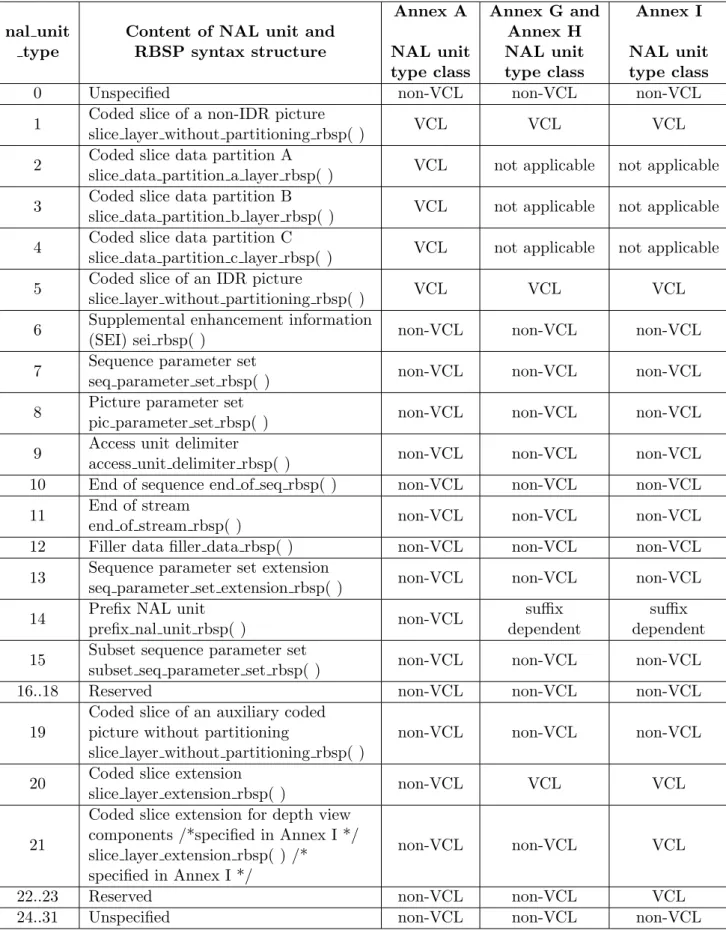
• nal unit type (5 bits): this field specifies the NALU payload type according to Table A.1

NAL UNIT Header NAL UNIT Payload

Forbidden

Bit NAL_REF_IDC NAL_UNIT_TYPE

3 4 5 6 7

0 1 2

Figure 2.4: NALU header structure

An Access Unit (AU) is a set of NALUs that once decoded result in a decoded picture made up of one or more slices. Each slice consists of a Slice Header and Slice Network Distributed 3D Video Quality Monitoring System 9

Data, that in turn is a series of coded macroblocks containing the information about its type (Intra, Inter), prediction information, QP and residual data.

The NALUs can be mapped by several transport layer schemes or encapsulated in a media file. This subject will be addressed in detail in Chapter 3.

2.1.2

HEVC

HEVC [4] coding standard was released on January 2013 by the ITU-T VCEG and the ISO/IEC MPEG, together forming the Joint Collaborative Team on Video Coding (JCT-VC). The main goal of this standard is to improve compression performance relative to other existing standards, promising a bitrate reduction by half for equal perceptual video quality, at the expense of increased computational complexity. HEVC is targeted to handle two new Ultra Hight Definition (UHD) standards: UHDTV1 ”4K” (3840 x 2160 pixels) and UHDTV2 ”8K” (7680 x 4320 pixels) with frame rates ranging from 23,976 to 120 Hz as a progressive scan, and use parallel processing architectures. This means that in the future service providers can deliver contents with double perceptual quality using the same bandwidth of today’s HDTV, or add services on the saved bandwidth due to HEVC use.

An HEVC compliant bitstream is produced by splitting each picture into blocks, this partitioning is reported to the decoder. The first picture of a sequence is coded using intrapicture prediction, the block of the remainnig pictures are typically coded using interpicture temporally predictive modes. The resulting residual signal from those two prediction schemes is transformed by a linear spatial transform, generating coefficients that are then quantized, entropy coded, and transmitted together with the prediction information.

So far this conceptual description is very similar to the one made about H.264, but although both standards employ the same hybrid approach (intra/ interpicture prediction and transform coding), HEVC has some interesting features that make it a standard for the future.

One of these features is its Quadtree Coding Structure (Figure 2.5). A quadtree is a tree data structure in which each node has exactly four children and are used to recursively partition a two-dimensional space by subdividing it into quadrants. So macroblocks in H.264 were replaced by Coding Tree Units (CTU) that in turn consists of a Coding Tree Block (CTB) containing luma, croma and syntax elements. The size of a CTB is chosen by the encoder and can be 64x64, 32x32 or 16x16 samples, generally larger sizes enable better compression. CTBs support partitioning into smaller blocks following the quadtree structure, generating Coding Units (CUs) and Coding Blocks (CBs). This means that a CTB can have one CU or be split into several CUs. A CU is in turn the root for the Prediction Units (PUs) and Transform Units (TUs). A Prediction Block (PB) can have the size of a CU or be split furthermore being the supported sizes 64x64,

32x32, 16x16, 8x8 and 4x4.

1656 IEEE TRANSACTIONS ON CIRCUITS AND SYSTEMS FOR VIDEO TECHNOLOGY, VOL. 22, NO. 12, DECEMBER 2012

Fig. 4. Subdivision of a CTB into CBs [and transform block (TBs)]. Solid lines indicate CB boundaries and dotted lines indicate TB boundaries. (a) CTB with its partitioning. (b) Corresponding quadtree.

further splitting is possible, as signaled by a maximum depth of the residual quadtree indicated in the SPS, each quadrant is assigned a flag that indicates whether it is split into four quadrants. The leaf node blocks resulting from the residual quadtree are the transform blocks that are further processed by transform coding. The encoder indicates the maximum and minimum luma TB sizes that it will use. Splitting is implicit when the CB size is larger than the maximum TB size. Not splitting is implicit when splitting would result in a luma TB size smaller than the indicated minimum. The chroma TB size is half the luma TB size in each dimension, except when the luma TB size is 4×4, in which case a single 4×4 chroma TB is used for the region covered by four 4×4 luma TBs. In the case of intrapicture-predicted CUs, the decoded samples of the nearest-neighboring TBs (within or outside the CB) are used as reference data for intrapicture prediction.

In contrast to previous standards, the HEVC design allows a TB to span across multiple PBs for interpicture-predicted CUs to maximize the potential coding efficiency benefits of the quadtree-structured TB partitioning.

F. Slices and Tiles

Slices are a sequence of CTUs that are processed in the order of a raster scan. A picture may be split into one or several slices as shown in Fig. 5(a) so that a picture is a collection of one or more slices. Slices are self-contained in the sense that, given the availability of the active sequence and picture parameter sets, their syntax elements can be parsed from the bitstream and the values of the samples in the area of the picture that the slice represents can be correctly decoded (except with regard to the effects of in-loop filtering near the edges of the slice) without the use of any data from other slices in the same picture. This means that prediction within the picture (e.g., intrapicture spatial signal prediction or prediction of motion vectors) is not performed across slice boundaries. Some information from other slices may, however, be needed to apply the in-loop filtering across slice boundaries. Each slice can be coded using different coding types as follows.

1) I slice: A slice in which all CUs of the slice are coded using only intrapicture prediction.

2) P slice: In addition to the coding types of an I slice, some CUs of a P slice can also be coded using interpic-ture prediction with at most one motion-compensated prediction signal per PB (i.e., uniprediction). P slices only use reference picture list 0.

3) B slice: In addition to the coding types available in a P slice, some CUs of the B slice can also be coded

Fig. 5. Subdivision of a picture into (a) slices and (b) tiles. (c) Illustration of wavefront parallel processing.

using interpicture prediction with at most two motion-compensated prediction signals per PB (i.e., bipredic-tion). B slices use both reference picture list 0 and list 1. The main purpose of slices is resynchronization after data losses. Furthermore, slices are often restricted to use a maxi-mum number of bits, e.g., for packetized transmission. There-fore, slices may often contain a highly varying number of CTUs per slice in a manner dependent on the activity in the video scene. In addition to slices, HEVC also defines tiles, which are self-contained and independently decodable rectan-gular regions of the picture. The main purpose of tiles is to enable the use of parallel processing architectures for encoding and decoding. Multiple tiles may share header information by being contained in the same slice. Alternatively, a single tile may contain multiple slices. A tile consists of a rectangular arranged group of CTUs (typically, but not necessarily, with all of them containing about the same number of CTUs), as shown in Fig. 5(b).

To assist with the granularity of data packetization, de-pendent slices are additionally defined. Finally, with WPP, a slice is divided into rows of CTUs. The decoding of each row can be begun as soon a few decisions that are needed for prediction and adaptation of the entropy coder have been made in the preceding row. This supports parallel processing of rows of CTUs by using several processing threads in the encoder or decoder (or both). An example is shown in Fig. 5(c). For design simplicity, WPP is not allowed to be used in combination with tiles (although these features could, in principle, work properly together).

G. Intrapicture Prediction

Intrapicture prediction operates according to the TB size, and previously decoded boundary samples from spatially neighboring TBs are used to form the prediction signal. Directional prediction with 33 different directional orientations is defined for (square) TB sizes from 4×4 up to 32×32. The

Figure 2.5: CTB partitioning and corresponding quadtree (adapted from [3])

Intra prediction specifies the 35 different prediction modes presented in Figure 2.6 (33 angular modes, a DC mode and an interpolation mode), much more than the 9 supported by H.264.

102 Rec. ITU-T H.265 (04/2013)

2. The general decoding process for intra blocks as specified in clause 8.4.4.1 is invoked with the chroma location ( xCb / 2, yCb / 2 ), the variable log2TrafoSize set equal to log2CbSize − 1, the variable trafoDepth set equal to 0, the variable predModeIntra set equal to IntraPredModeC, and the variable cIdx set equal to 1 as inputs, and the output is a modified reconstructed picture before deblocking filtering.

3. The general decoding process for intra blocks as specified in clause 8.4.4.1 is invoked with the chroma location ( xCb / 2, yCb / 2 ), the variable log2TrafoSize set equal to log2CbSize − 1, the variable trafoDepth set equal to 0, the variable predModeIntra set equal to IntraPredModeC, and the variable cIdx set equal to 2 as inputs, and the output is a modified reconstructed picture before deblocking filtering.

8.4.2 Derivation process for luma intra prediction mode

Input to this process is a luma location ( xPb, yPb ) specifying the top-left sample of the current luma prediction block relative to the top-left luma sample of the current picture.

In this process, the luma intra prediction mode IntraPredModeY[ xPb ][ yPb ] is derived. Table 8-1 specifies the value for the intra prediction mode and the associated names.

Table 8-1 – Specification of intra prediction mode and associated names

Intra prediction mode Associated name

0 INTRA_PLANAR 1 INTRA_DC

2..34 INTRA_ANGULAR2..INTRA_ANGULAR34 IntraPredModeY[ xPb ][ yPb ] labelled 0..34 represents directions of predictions as illustrated in Figure 8-1.

17 16 15 14 1 3 12 1 1 10 9 8 7 6 5 4 3 2 18 19 20 21 22 23 24 25 26 27 28 29 30 31 32 33 34 0 : Intra_Planar 1 : Intra_DC

Figure 8-1 – Intra prediction mode directions (informative)

IntraPredModeY[ xPb ][ yPb ] is derived by the following ordered steps:

1. The neighbouring locations ( xNbA, yNbA ) and ( xNbB, yNbB ) are set equal to ( xPb − 1, yPb ) and ( xPb, yPb − 1 ), respectively.

Figure 2.6: HEVC prediction modes [4]

For inter prediction modes, non-square modes are allowed although a PB inter frame cannot have the 4x4 size.

To generate a prediction for the current block the encoder must determine the best PB size to use by testing all prediction modes at all PB sizes available and then choose the best combination, based on Rate distortion Optimization (RDO). For example, to process intra prediction mode decision, the encoder needs to measure the values of distortion for each one of the 35 prediction modes and for every level of the PU subtree. Checking all these possibilities is a very demanding computational task and prove to be impractical for real-time encoding, so there are several schemes to enable smart mode decision without running the totality of the encoding process described in [17] for fast Intra Prediction mode decision, and [18] for Coding Tree Depth complexity reduction.

This standard is receiving great attention from research groups around the world, and although it is outside of the scope of this work, in the near future a similar approach could be taken, to develop a system similar to the one being presented, to monitor HEVC video quality

2.2

3D Video Coding

3D video is commonly known as a type of visual media that gives the viewer the per-ception of depth. To accomplish this, a whole system, from acquisition, to storage and display has to be in place while keeping interoperability and compatibility with existing 2D video infrastructures.

For professional 3D video capture, typically setups with 2 or 3 cameras are used. The problem associated with multi-camera systems are temporal synchronization, geometrical calibration [19] and colour balance between all cameras. There are also camera setups equipped with depth sensors capable of depth enhanced 3D video. This means that 3D video formats can be divided into two main classes [20]: video-only formats and depth-enhanced formats. Video-only formats can be further divided into Classical Stereo Video (CSV) with two views, Mixed Resolution Stero (MRS) video with one of the views spatially sub-sampled and Multi-View Video (MVV) with more than two views. In turn, depth-enhanced formats can also be sub divided into Video plus Depth (V+D), Multi-View Video plus Depth (MVD) and Layered Depth Video (LDV). The advantage to the inclusion of depth or disparity information into these video formats is that 3D video reproduction can be adapted to any display, since all views are synthesized at the decoding stage.

For the scope of this work only MVV coding schemes will be addressed. Apart from support for 3D video MVV also enables free-viewpoint video, were the video direction can be interactively changed and presented on a 2D display. All these features represent great amount of data that needs to be efficiently compressed, while keeping backwards compatibility.

2.2.1

H264/AVC Multi-View video Coding

The straightforward approach to encode MVV is to encode each one of the views separ-ately treating them as independent videos ensuring backwards compatibility. Although possible, such approach proves to be very inefficient when comparing it to H264/AVC extension for Multi-View video Coding (MVC). Annex H of [16] describes all key features and syntax elements of this standard.

Inter-view prediction is the concept introduced in MVC, that is responsible for ex-ploiting spatial and temporal redundancy for compression purposes. Since cameras on a

multiview scenario capture the same scene from nearby viewpoints there is great inter-view redundancy (Figure 2.7), and temporal redundancy is also present [5].

The encoder is applied to the view sequences simultaneously enabling inter-view predictive coding, resulting in dependant bitstreams to which information about camera parameters may be included.

I B B B B B B B I B P B B B B B B B P B P B B B B B B B P B P B B B B B B B P B Camera 1 Camera 2 Camera 3 Camera 4 TIME

Figure 2.7: Picture prediction relation in MVC (adapted from [5])

To make backwards compatibility possible the MVC design states that the com-pressed multiview stream must include a baseview bitstream, coded independently from the other views. The remaining specifies a NALU header extension for NALUs of type 14 and 20 (Table A.1, Annex A). Since these NALU types were reserved for this pur-pose, decoders conforming to one or more of the profiles specified before MVC, thus not supporting it, will be capable of reproducing 2D video corresponding to the base view. Any unknown information is discarded, keeping backwards compatibility.

NAL units created using the MVC profile have additional fields to the ones in Section 2.1.1 described in [21]. They are illustrated in Figure 2.8 and described bellow:

• (R) reserved zero bit (1 bit): reserved for future extension. Must be 0 and should be ignored at reception;

• (I) idr flag (1 bit): specifies whether the view component is a view instantaneous decoding refresh picture;

• (PRID) priority id (6 bits): a lower value indicates higher priority in relation to other NALs;

• (VID) view id (10 bits): this component corresponds to the identifier of the view the NALU belongs to;

• (TID)temporal id (3 bits): temporal layer identification. A video bitstream can have several temporal layers where all NALUs of one layer form a valid bitstream with a given frame rate. The higher the temporal layer is, higher the frame rate; • (A) anchor pic flag (1 bit): this field signals whether the view component is an

anchor picture;

• (V) inter view flag (1 bit): specifies if the view component is used for inter-view prediction;

• (O)reserved one bit (1 bit): reserved for future extension. Must be 1 and should be ignored at reception.

The contents and structure of the NALU fields is of great importance for the project, since they will be used for network bitstream parsing purposes and data retrieval. NALUs contain actual video data so their header information is used to categorize the type of content they are carrying, and for this case, the information to retain is nal ref idc and nal unit type(defined in Section 2.1.1). The nal ref idc field specifies the importance of the content, and nal unit type specifies if the payload is part of the VCL (Type 1,5 and 20) and if the NALU contain an Instant Decode Refresh IDR picture (Type 5), meaning that this NALU contains a payload that contains reference information and will force decoder refresh. These combination of the content of these two fields will help determine if the content of a network packet is from an I, B or P slice. From MVC specific fields the ones used are the idr flag and view id, but for confirmation purposes only since there are other ways to determine if a bitstream passing through the network is from a 3D video stream or to determine if a picture is an IDR picture.

NAL UNIT Header NAL UNIT Payload

3 4 5 6 7

0 1 2 0 1 2 3 4 5 6 7 0 1 2 3 4 5 6 7 0 1 2 3 4 5 6 7

F NRI Type R I PRID VID TID A V O

Video Transport

This chapter describes standardized methods to broadcast/transmit video over IP net-works and their characteristics. Also video encapsulation methods are explained, giving more emphasis to the encapsulation structure used in this project.

3.1

Video Packetization

3.1.1

Internet Protocol

The Internet Protocol [22] is datagram transport protocol used to relay data across networks, and is the base of the internet. IP packets consist of a header containing ad-dressing and control information for packet routing through the network, and a payload, that consists of the data to be transmitted. The payload can carry several protocols for data streaming such as RTP and UDP.

3.1.2

User Datagram Protocol

The User Datagram Protocol (UDP) protocol [23] enables computer applications to send messages to other hosts on an IP network without prior communications to set up a transmission channel. It provides checksums for data integrity and port numbers for addressing different functions at the source and destination of the datagram. UDP is used in situations where error checking and correction is not a necessity or is done by the application, avoiding the overhead at the network interface level. Time-sensitive data transmission such as video use this protocol because dropping packets is preferable over waiting for delayed ones.

3.1.3

Real-time Transport Protocol

The Real-time Transport Protocol (RTP) protocol [24] provides end-to-end delivery ser-vices for data with real-time characteristics (video and audio). It provides payload type identification, sequence numbering, time-stamping and deliver monitoring. Normally it runs on top of UDP making use of its characteristics, and can be used with other suitable underlying network or transport protocols.

Since RTP doesn’t provide any mechanism to guarantee quality-of-service, timely or out-of-order data delivery, but the included sequence numbers allow the receiver to reconstruct the packet sequence and detect packet losses.

H.264 video carriage over RTP is defined in [25], were NALUs are mapped into the payload accordingly.

3.1.4

MPEG 2 Transport Stream

This packetization method is described in more detail than the previous ones because of its importance for project development.

MPEG 2 Transport Stream (MPEG2-TS) [26, 27] was first specified in MPEG-2 Part 1. Due to its structure and flexibility is still in use and provides a way to transmit several types of data (audio and subtitles in several different languages, 3D video, ... ) in the same stream while being compatible with all devices that may not support all its features.

Before transmitting the different sources of data must be packetized and MPEG2-TS does this by multiplexing data. Packet multiplexing is simply interleaving packets of data from several elementary streams one after another to form a single MPEG2-TS stream.

Synchronization is very important in multimedia and MPEG2-TS has several means to maintain it between the elementary streams that are being decoded. This is achieved by using Time Stamps and Clock References, that are added to the MPEG2-TS stream at the time of multiplexation. There are two types of Time Stamps (Decoded Time Stamp and Presentation Time Stamp) and they refer to a particular moment when a video picture or sound frame should be decoded and presented on the output device. They are represented by a 33 bit data field containing a time reference indicated by the System Time Clock. The Clock References (42 bit data field) are used by the decoder to update their own clock reference.

Packetized Elementary Streams

Elementary Streams (ES) are compressed data from a single source and all the attached auxiliary data needed for synchronization and identification of the source (NALUs in H.264). These sources are packetized into Packetized Elementary Streams (PES) that

can be of fixed or variable length and it is comprised of a header and the stream data (payload).

The PES packet structure can be seen in Figure 3.1. Its fields are described bellow: • start code prefix : 24 bits all 0 except for the last one;

• stream id : 8 bits ranging from 0xBD to 0xFE and defines type of stream or an ID for different streams of same type;

• PES packet lenght : 16 bits stating the number of bytes that follow. For video packets, this field can have a value of 0 indicating an unspecified length;

• padding bytes : Bytes equal to 0xFF that are discarded at the decoder; • marker bits : 2 bits with fixed valued bits usually all 1s ;

• PES scrambling control : 2 bits indicating scrambling mode;

• PES priority : 1 bit indicating that a PES packet has higher priority;

• data alignment indicator : 1 bit indicating if the payload starts with a video Start-Code or audio sync-word ;

• copyright : 1 bit indicating if the PES has copyrights; • original or copy : 1 bit indicating if stream is original;

• PTS DTS flags : 2 bits. 0 (decimal) indicates that there isn’t any PTS or DTS. 3 indicates presence of both and 2 means that only PTS is present;

• ESCR flag : 1 bit to indicate presence or a clock reference in PES header ; • ES rate flag : 1 bit to indicate if bitrate value is present in PES header; • DMS trick mode flag : 1 bit indicates if there is an 8-bit trick mode field; • additional copy into flag : 1 bit indicates additional copyright information ; • PES CRC flag : 1 bit to indicate presence of a CRC is present;

• PES extention flag : 1 bit indicating if PES header extension fields are present; • PES header data lenght : 8 bits containing the length of the optional PES

header extension fields. ;

• PTS : Presentation Time Stamp defines when the output device should present the decoded information;

PES_packet_data Optional PES HEADER PES packet length stream_id start_code _prefix 24 8 16 marker_ bits PES_ scrambling_ control PES_ priority data_ alignment_ indicator copyright original_ or_ copy Flags: PTS_DTS; ESCR; ES_rate; DMS_trick_mode; additional_copy_into; PES_CRC; PES_extention. PES_header

_data_length Optionalfields stuffingbytes

ESCR ES_rate mode_trick_ control additional_ copy_info previous_ PES_ packet_CRC DTS PTS PES extension 2 2 1 1 1 1 8 8 n*8 33 33 42 22 8 7 16

...

Figure 3.1: PES packet structure

• DTS : Decoding Time Stamp defines when a stream should be decoded (may have a value of 0);

• ESCR : Elementary Stream Clock Reference; • ES rate : Bitrate of a PES Stream;

• trick mode control : Indicates the trick mode applied to the video (fast forward, pause, rewind, ...) ;

• additional copy info : contains copyright information;

• previous PES packet CRC : 16 bits containing information about previous PES packet (excluding header fields);

• extension data : can include buffer sizes, sequence counters, bitrates...; • stuffing data : no more than 32 stuffing bytes are allowed in one PES header; • PES packet data : Bytes of data from the elementary stream;

All fields from this packetization technique had to be described due to their content or structural importance in data parsing procedures. The start code prefix helps to identify if a PES packet header is present, followed by the stream id that identifies type of data the PES packet is carrying (audio, subtitles, video ...) and for the case of video content the stream id is equal to 0xe0. PES packet lenght is one of the essential fields to be retrieved for analysis, and if is 0, action needs to be taken to determine this parameter in an other way. PTS and DTS are also used to determine the elapsed video time passing through the network. Please note that two consecutive packets containing a PTS must not be more than 700 ms apart. PES header data lenght is used to determine where the payload (NALU) data starts.

Program Streams

Program Streams (PS) are comprised of packs of multiplexed data. These packs contain a header followed by a variable number of PES packets from several elementary stream sources each one with an unique stream id. Additionally to PES packets, PS Packets also contain descriptive information called PS Program Specific Information (PS-PSI), that defines the program and its parts storing, for example, where I-pictures are stored en-abling random access to several points of the stream. Program Streams are indicated for media storage or transmission over networks where reliability possible video degradation is not a problem.

Transport Streams

This stream type is suitable for transmission networks that suffer from occasional trans-mission errors. It is also comprised of multiplexed data from PES packets and some more descriptive data.

Generally variable length PES packets are further packetized into fixed 188 bytes long Transport Stream (TS) packets. This division into constant length packets makes error detection and recover easier.

A TS packet contains a TS Header, optionally secondary data called Adaptation Field and some or all data from a PES packet. The Header contains synchronization information, a Packet Identifier (PID) and information on timing and error detection, all this described in detail below:

• sync byte: 8 bits. Fixed value of 0x47;

• transport error indicator: 1 bit indicating the presence of an uncorrectable bit error in the current TS packet ;

• payload unit start indicator 1 bit signalling the presence of a new PES packet or a new TS-PSI Section ;

• transport priority: 1 bit stating higher priority over other packets ; • PID: 13 bits for Packet Identification;

• transport scrambling control: 2 bits to indicate presense of the scrambling mode of the packet payload;

• adaptation field control: 2 bits to signal the presence of an adaptation field or payload ;

• continuity counter: 4 bits. One for each PID incrementing every TS packet ; • pointer field: 8 bits indicates the number of bytes until a new TS-PSI Section ; Network Distributed 3D Video Quality Monitoring System 19

Additionally to the above fields exist some more optional ones which presence is sig-nalled by the adaptation field control. They are called Adaptation Field contains System Time Clock timing information called Program Clock Reference (PCR). This in-formation is important for decoder synchronization and is transmitted with a periodicity of at least 100 ms. The fields are described bellow:

• adaptation field lenght: 8 bits indicating the number of bytes following; • discontinuity indicator: 1 bit signals discontinuity in clock reference or

continu-ity counter ;

• random access indicator: 1 bit if the next PES packet starts a video or audio sequence;

• elementary stream priority indicator: 1 bit stating higher priority; • PCR flag: 1 bit. PCR is present;

• OPCR flag: 1 bit. Original PCR is present;

• splicing point flag: 1 bit indicating that a splice countdown field is present; • transport private data flag: 1 bit. Adaptation field has private data;

• adaptation field extension flag: 1 bit flag signaling presence of extension fields; • program clock reference (PCR): 33 bits, value based on a 90kHz reference

clock + 6 padding bits + 9 bits extension based on a 27 MHz clock;

• original program clock reference (OPCR): same size as PCR, used to extract a single program from a multiprogram TS;

• splice countdown: 8 bits with the number of remaining TS packets (same PID) until the end of an audio frame or video picture;

• transport private data legth: 8 bits stating the number private data bytes fol-lowing;

• private data bytes: private data;

• adaptation field extension lenght: 8 bits. Number of bytes of the extended adaptation field;

• stuffing bytes: variable number of 8-bit values of 0xFF, to discarded by the encoder.

sync_ byte transport_ error_ indicator payload_ unit_start indicator continuity_ counter transport_ priority PID transport_ scranbling_ control adaptation_ field_ control Adaptation field splice_ countdown transport_ private_data _length private_ data_bytes OPCR PCR optional fields 8 1 1 1 13 2 2 4 42 42 8 8 7 16

...

payload

HEADER HEADERTS

payload

payload

188 bytes

Flags: PCR; OPCR; splicing_point; transport_private_data; adaptation_field_extension; stuffing_ bytes optional fields 8 1 1 1 5 3 flags

Figure 3.2: TS packet structure

From these fields sync byte helps confirm that a TS packet is present, payload unit start indicator signals that a PES packet header is present, that is usually also followed by a NALU

header. PID identifies a packet that contains a certain type of stream, for 3D each one of the views has a different PID. The continuity counter is used to identify packet loss events and determine the number of packet losses per view. Adaptation field lenght and adaptation field extension lenght are used to locate where in the bitstream is the start of the payload without doing a byte-by-byte sweep.

There are three special TS streams (TS - Program Specific Information)that contain additional information such as program descriptions and assignments of PES and PIDs. The first type of stream is the Program Association Table (TS-PAT), and always has a PID equal to 0, and is the first stream to be transmitted. For each program the TS-PAT defines the association between the program number and a PID. Another special stream is the Network Information Table, that carries data describing and characterizing the network carrying the TS. Since this data is dependent of network implementation it is considered Private data. The third type of stream are Program MAP Tables that carry information about each one of the programs in the transmission stream such as the assignments of the unique PID values for each of the PES streams. Although these types of TS streams could be useful to this work they were not used or implemented, since MVC streams can be identified without them, so implementing identification and parsing of these TS streams would not add any value to the work, hence the lack of description.

U D P H ea de r TS/RTP/UDP/IP Packet TS/UDP/IP Packet RTP/UDP/IP Packet IP H ea de r U D P H ea de r R TP H ea de r TS H ea de r TS H ea de r TS H ea de r IP H ea de r U D P H ea de r TS H ea de r TS H ea de r TS H ea de r IP H ea de r R TP H ea de r N AL U H ea de r

Figure 3.3: Comparison between transport methods

3.1.5

MPEG2-TS transport methods

One of the two methods used to transport MPEG2-TS over IP networks is to carry these packets over RTP (specified in [28] and [29] ).

The other method, and the one being used in the scope of this work, selects a number of TS packets and adds them to the payload of the UDP datagram. For Ethernet networks the Maximum Transmission Unit (MTU) has 1500 bytes, so 7 TS packets may be transmitted on the same UDP packet (1500/188 ≈ 7). Comparison of the structure of the several transport methods can be seen in Figure 3.3.

3.2

3D MPEG2-TS encapsulation

Prior to transmission MVC data has to be encapsulated into MPEG2-TS (Figure 3.4). This is done by splitting the MVC encoded bitstream into ES from the same view, and then encapsulate each one into PES packets. The resulting PES packets are in turn split into pieces with TS packet payload size and encapsulated. Since the size of a PES packet is variable, the number of TS packets needed to contain it also varies, and if the remainder of a PES packet is not enough to fill one TS, the rest of the available space is filled with 0xFF. This happens because a PES must start immediately after the TS header, thus not allowing remainder free TS payload space to be filled with a new PES packet header. For each one of the views present (two in 3D) TS packets have a different

PID to distinguish all the views, treating them as separate video streams.

...

...

...

...

...

...

...

...

...

...

...

Figure 3.4: Illustration of MVC bitstream encapsulation into TS

To identify a 3D video stream at network level one must know the meaning of each field of the bistream. Since a TS packet can carry very different data types (several video views, audio channels and subtitles of different languages) by multiplexing their sources into one single stream, data parse can be a very complex task since it involves several variables from several packetization hierarchies.

3D Video Qualiy Models

The importance of video quality measurement over IP networks is increasing due to the exponential growth of available streaming services to the consumer. Understanding the impact that packet loss events have in perceived video quality is therefore an important matter. In [30] a brief analysis of the H.264 MVC performance over error prone IP networks using RTP packetization is conducted, and in [31] the effects on video quality of corrupted H.264 bitstreams is evaluated. The main methods to evaluate video quality are subjective and objective techniques, being the former based on human observers that evaluate the video quality of samples that are presented to them. Results from the subjective methods are then used to compute Mean Opinion Score (MOS) and other statistics. However, these results are subject to great variations due to environmental conditions (lighting, viewing distance, shown video samples) and observer conditions [32, 33]. Also, they are expensive and take a fair amount of time to produce results; An objective video quality evaluation method enables automatic estimation of user perceived video quality without the need of any human intervention thus making it a faster, reliable and cheaper solution.

In objective techniques a set of quality related parameters of a video are gathered and processed to generate an objective quality metric capable of predicting the MOS. Depending on the information available from the original video, the objective methods can be divided into three categories [34]:

• Full-Reference (FR): the original video is available to be used for comparison with the distorted one. This proves to be impractical in cases were video quality needs to be monitored in remote locations, were the reference is not available; • Reduced-Reference (RR): only some features of the original video are needed

to determine the video quality. Although the needed data is much less than in the FR methods, it has the same problem and is not an option when trying to measure the quality at any point of the transmission channel;

• No-Reference (NR): these methods do not use any reference to compute video quality. This represents a great advantage over the other two categories since Network Distributed 3D Video Quality Monitoring System 25

it allows video quality assessment at any point of a transmission network. This category can be further divided into two [35]:

– No-reference pixel-based: the video quality is estimated by using the de-coded video;

– No-reference bit stream-only: the video quality estimation is done without completely decoding the video to obtain decoded pixels. The needed inform-ation is extracted from packet headers at the network-layer, as in the scope of this work.

In [34] the most used quality metrics are detailed: Mean Square Error (MSE), PSNR and Structural Similarity (SSIM) [36] whose mathematical expressions are Equations 4.1 , 4.2 and 4.3 respectively. M SE = 1 N n=1 X N (Xn− Yn)2 (4.1) P SN R= 10 log10 L2 M SE (4.2) SSIM(x, y) = (2uxuy+ c1)(2σxy + c2) (u2 x+ u2y + c₁)(σ2x+σ2y+ c2) (4.3)

Where for the MSE Xn and Yn are the pixel values of the original and distorted

frames, and N is the total number of pixels in a frame. For the PSNR L is the maximum pixel value in a frame. Although these metrics are widely used, they have no correlation with the human visual system meaning that the results produced by them and video quality perception from a human are far from each other, thus they cannot be used in 3D video quality assessments.

The SSIM uses structural information from the video, approximating a video quality assessment metric to the perception of the human visual system. x and y are the original and the distorted frame information, ux and uy are the mean of x and y. σx , σy and

σxy are the variance of x, y and the covariance between x and y. Finally c1 and c2 are

constants to avoid the denominator becoming very close to 0.

4.1

NR Quality Models

There are several quality models reported in the scientific literature for image or video perceived quality prediction.