The relationship between changes in
debt levels and firms’ stock returns
within emerging markets.
Evidence from Brazil
Table of Contents
I – Introduction………...3
II - Literature review………..5
III – Methodology and Data……….10
IV – Empirical Results...………...12
V – Conclusion………...24
A B S T R A C T
I document a positive effect of both, positive and negative changes, of a firm’s leverage ratio on its stock returns for the Brazilian emerging market for the period of ranging from 2000 to 2016. I find positive alphas which indicates the existence of abnormal returns and try to explain them using asset pricing models. Additionally, I use the Event study methodology to quantify both the abnormal and cumulative abnormal returns. Furthermore, I run time series regressions for each company in the Brazilian index with available data to test the CAPM and Fama French 3 factor models and include other variables to possibly explain the abnormal returns.
I - Introduction
Leverage is commonly acknowledged as one of the primary sources of financial risk. A firm’s capital structure decision is therefore, vital, as altering the debt-to-equity ratio can impact the entity’s financing capacity, its risk and its cost of capital influencing investment and strategic decisions which ultimately will impact shareholders wealth.
From a traditionalist’s perspective an optimal debt level exists where the marginal benefit of debt, which is the tax shield from employing debt, is equivalent to the marginal cost of debt, which are increases in direct and indirect financial distress costs. On the other hand, Modigliani and Miller (1958, henceforth MM) argued that, in a frictionless efficient market world, the value of the firm and its cost of capital are independent of the capital structure. This suggests that return on equity is an increasing function on leverage, since the risk for equity holders increases, thus there will be a demand for a higher return on their stock as compensation. Such that, according to one perspective, firms try to maintain an optimal (target) capital structure responding to disruptions through rebalancing their leverage ratio back to the optimal level or we can have firms that dynamically adjust their capital structure. Despite those capital structure theories, past literature provides mixed empirical evidence concerning the role of leverage and stock returns. Among various studies, Masulis (1983) and Bhandari (1988) found that stock returns are positively associated with leverage. Fama and French (1992) later discovered a negative relationship between book leverage and returns, which was reinforced by George and Hwang (2010) and later by Muradoglu and Sivaprasad (2012).
This paper will assess the repercussions of an aggregate change in the capital structure on stock returns. Majority of the existing papers in this area tend to focus on the market’s reaction to changes in the capital structure during events of stock/debt issuances or share buybacks. Other elements, in addition to the ones listed before, can impact a firm’s capital structure choice. These
include dividend payments, provisions of trade credit or payment and use of existing credit lines. Therefore, I examine the overall effect of the change in leverage levels on stock returns. Moreover, I intend to study the relationship between the impact of leverage on returns in an emerging market. Specifically, the chosen emerging market for this study is Brazil.
Theoretically, a hypothesis can be formed with the expectation of the stock price decreasing with an increase in the leverage ratio, as implied by Myers (1977). However, there are mixed empirical results Bhandari (1988) and Fama and French (1992). Extending the analysis to an emerging market, where there are little studies available in this area, I study how the companies, which are constantly challenged and subjected to high volatility, respond to variations in their debt levels with the aim to help managers and investors take decisions.
In addition, I conduct an event study to study the firms’ decisions regarding leverage change in the short-term and its impact on stock returns. For that, my objective is to emphasize the existence of short-term abnormal returns when firms reach their maximum leverage ratio during the period under analysis. Note that, firms can engage in short-term leverage increases in order to pursue positive NPV projects.
The remainder of this paper is organized as follow: Section II provides this paper’s contribution relative to the existing literature, namely the research content and its findings as well as the key concepts associated with the subject matter of this paper. Section III presents the methodology used and an explanation for the selection of the most suitable companies for this analysis. Section IV presents the data and the empirical results and Section V concludes this paper.
II – Literature review
There is extensive literature concerning optimal capital structure but there is little empirical evidence regarding the impact of changes in leverage on stock returns in an emerging market. The financing decision is a critical concept in corporate finance. Many studies have been developed in the finance literature to determine the factors that influence the capital structure choice and, therefore, present conclusions on the optimal level of debt. This view argues that firms respond to disruptions in their optimal capital structure by rebalancing their leverage ratio back to their optimal level, where a firm must equaalize its marginal cost of debt to its marginal benefit. This is dependent on the entity and its surroundings, and may differ greatly according to the industry it operates in, the country and firm-specific characteristics. The discussion regarding the impact of debt commenced with the pioneer study of Modigliani and Miller in 1958, which raised questions regarding the relevance of capital structure on total firms’ value. It was initially concluded that in a perfect market world with no taxes, agency costs and bankruptcy costs, there is no effect on a firms’ value or its weighted average cost of capital if the capital structure is altered. However, in that study some naïve assumptions were made regarding the inexistence of corporate taxes and no risk of bankruptcy, which led to the addition of counter studies claiming MM (1958) assumptions were unrealistic. Such market does not exist in reality since firms have to pay corporate taxes and are subject to the risk of bankruptcy and its costs, when debt is increased to an unsustainable level. Since then, many other studies were developed and extended to include new variables that were not considered by the original authors, all with the same idea that there should be an optimum level of debt versus equity that maximizes the value of the firm.
Thus, Modigliani and Miller (1963), presented the same model but this time expanded their assumptions to include corporate taxes. Proposition I concludes that there is a positive relationship between firm value and leverage, which was exclusively attributed to tax shields. The rationale is
that debt is tax deductible and thus, by utilizing debt, the firm enjoys an interest tax shield. Moreover, with an increase in the amount of debt used, the market value of the firm would increase by the present value of the interest tax shield. The second proposition of Modigliani and Miller (1958, 1963) stated that increasing financial leverage would lead to an increase in expected stock returns. Note that the theoretical impact of this proposition on corporate finance is immense but the original sample used was very limited (empirical tests exclusively in the utilities and oil and gas industries). Therefore, further empirical research utilizes much larger data samples, which have resulted in mixed empirical evidence.
Korteweg (2004) used a time series approach with Fama and French’s 3-factor asset pricing model, and concluded that stock returns decline when gearing (debt-to-equity) increases.
Moreover, Dimitrov and Jain (2008) focused on the change in leverage as a result of the economic performance and not due to growth, M&A or sudden changes in capital structure. They contested that the level of debt employed by a firm can offer better information to the market regarding the firm’s economic performance, compared to information from earnings and cash flows. Thus, they concluded a negative relationship between the level of debt and risk-adjusted stock returns. On the other hand, Hamada (1972) and Bhandari (1988) show that returns increase in leverage. Bhandari (1988) concluded that expected returns on common stocks are positively related to the debt-to-equity ratio, controlling for the beta and firm size, and unrelated with sensitive variations in the market proxy nor estimation technique.
Additionally, in 2008, Gulnur and Sheeja studied all non-financial firms covering all different risk classes (sectors) and showed that returns increase in leverage for one risk class (utilities), in line with the findings of Miller and Modigliani and Bhandari (1988), but decrease in leverage for others, consistent with the work of Korteweg (2004), Dimitrov and Jain (2008), and Penman (2007). It is important to note that the risk class has a strong impact on the relationship
between leverage and stock returns. In the utilities sector, a highly regulated industry, firms may be able to increase their leverage as a result of the increased debt holder protection through the regulation, thus there is a higher concentration of high leverage ratios. Note that they found that the contradicting empirical results in literature are mainly due to restrictions in the samples used.
Nevertheless, this does not necessarily mean that corporations should always seek to use the maximum possible amount of debt in their capital structures, despite its tax advantage. Other forms of financing, for instance, retained earnings, may be cheaper than debt, even when the tax status of investors under the personal income tax is taken into account. (Modigliani and Miller, 1963:442). However, in Miller’s revision in 1977, which accounted for personal income taxes, a conclusion was drawn that the differential tax impact on debt and equity holders shrinks the previously glorified interest tax shield.
Furthermore, Baxter (1967), Stiglitz (1972), Kraus and Litzenberger (1973) and Kim (1978) added bankruptcy costs, Jensen and Meckling, (1976) and Miller (1977) included agency costs, and Myers introduced asymmetric information, for which the results suggested that one should consider the costs and benefits of debt in order to find the optimal capital structure of one’s firm, maintaining the opinion that an optimal capital structure may exist. Moreover, Jarrell and Kim (1984) and Titman and Wessels (1985) strongly support that bankruptcy costs and agency costs play a crucial role in leverage and optimal capital structure.
De-Angelo-Masulis (1980) concluded that every firm will have a distinct optimum leverage point including or excluding leverage related costs. Their model suggested that a firm’s optimal debt-to-equity ratio is associated with its industry, mainly due to different tax rates across different industries (consistent with Vanils 1978 and Siegfried, 1984) and in 1983 contested that when firm’s issue debt closer to the industry average, from below, the market reacts more favorably, when compared to firms that move away from the industry average.
Hence, these studies that added new elements to the original MM (1958) study resulted in the development of two major capital structure theories: trade-off and pecking order theories of capital structure. The former theory assumes that firms will choose their capital structure on the basis of the tax benefits of debt and bankruptcy costs in order to achieve an optimal debt ratio. The latter, as proposed by Myers (1984) is a theory that explains the preferential choice over funding sources, whereby firms will select internal funding over external financing whenever possible. This is due to information asymmetries associated with equity financing, thus a firm’s least preferred choice and therefore, one that is mostly avoided is equity issuance. Thus, this developed a financing hierarchy with preference to retained earnings, then debt, and finally, equity. It is important to mention that, Frank and Goyal (2003) showed that this theory was more consistent in the 1970s and 1980s, whereas in the 1990s, it was less applicable, as explained by Huang and Ritter (2007) who argued that the poor performance in recent years is justified by the decline in the equity risk premium.
More recently, a new theory has been challenging the two previous concepts. The notion is that firms engage in market timing (issuing equity when the equity market is perceived to be more favorable and market-to-book ratios are relatively high), stating that firms prefer external equity when the cost of equity is low and prefer debt, otherwise. Baker and Wurgler (2002) support this view by providing confirmation that market timing has a persistent impact on corporate structure. An alternative viewpoint, relative to recent empirical studies, is that firms dynamically adjust their capital structure, implying that an entity’s history is indeed a more important determinant of its capital structure than firms’ characteristics that proxy for the costs and benefits of debt versus equity.
Welch (2004) maintains that equity returns are negatively correlated with market-based debt ratios, if firms, subsequent to episodes of stock price variations, do not rebalance their debt
ratios. Welch (2004) investigates whether firms offset stock return-induced changes in capital structure and deduced that firms do remarkably little to readjust their leverage for the effect of share price fluctuations. Note that firm’s observable debt ratios vary closely with movements in their own share returns, whereas equity price shocks have an ongoing impact on capital structures. Thus, a conclusion is drawn that the primary determinant of capital structure changes are stock returns. He also found that 40% of the variation in debt ratios can be explained through the implied effect of stock returns, for a sample of US firms.
More recently, Drobetz and Pensa (2015) discovered results that were consistent with Welch’s (2004) results for US data. He found roughly 60% and 50% of the 1-year and 5- year variation in leverage, respectively, can be explained by return-induced changes in the capital structure.
III - Methodology
MM (1958) define leverage as the ratio of the market value of bonds and preferred debt to the market value of all securities. The literature measures capital structure in two ways: i) book leverage, which equals the book value of total liabilities divided by the book value of total assets and ii) market leverage, which equals the book value of total liability divided by the sum of the book value of total liabilities and the market value of shareholders’ equity. In this study, I focus on measuring leverage according to book leverage since changes in market leverage can be mechanically related to stock prices. Moreover, I define leverage change as the change in book leverage from the previous quarter. Previous studies used several definitions for returns. Arditti (1967) defined returns as the geometric mean of returns. He found a negative, although insignificant, relationship between leverage and stock returns. I represent returns to shareholders as the compounded return between two quarters.
According to Bhandari (1988) a firm’s beta alone has been found to be inadequate in explaining the expected common stock return. Therefore, Bhandari introduced a new variable, DER (debt-to-equity ratio), to explain the expected common stock returns since there is a need for a new variable to account for market imperfections.
Through an assessment of various empirical papers, one statistical method has commonly been used to establish a relationship between stock returns and debt, the Ordinary Least Squares (OLS) regression method. I investigate the impact of stock returns on the capital structure dynamics of a representative Brazilian sample of 45 firms over the period from 2000 to 2016, controlling for excess return of the market (CAPM), firm size and value, which was measured by the returns of the Fama-French size and value factors (SMB and HML) and momentum, which was measured by the returns of Carhart 4 factor model (UMD). The explanatory power of capital structure and other financial variables identified in previous academic literature are tested to see the impact on stock returns. Such that, statistical tests are performed using a unit root test to control for stationarity and multicolinearity of the data. Moreover, heteroscedasticity and serial autocorrelation of the error terms in the regression equation were controlled using White’s and Breusch-Pagan-Godfrey, respectively.
Data
Quarterly financial data, covering the years 2000 to 2016 for 65 listed firms in Brazil’s index Ibovespa, were collected from Thomson Reuters and Economática. The reason why data was collected for that period was to include a macro-shock (2008 global crisis) to try to understand how firms in an emerging market reacted to it. Moreover, as I am using quarterly data, a large number of years were needed in order to have a significant sample to proceed with the empirical analysis. Following prior literature, all financial companies, including banks, investment companies, insurance and life assurances, were excluded from the data sample because of the level of debt on
their balance sheet, which does not carry a similar financing definition as it would for ordinary non-financial firms. The analysis of these financial firms should be treated in a different way, and so are not covered in this study. Firms with non-positive book values of equity and negative total liabilities are excluded from the sample, because these firms have extreme leverage ratios: greater than one or less than zero. Due to the filtering process, the selected sample is not free of survivorship and selection bias. In some circumstances, there might be missing values in the time series of firms characteristics used to run the regressions.
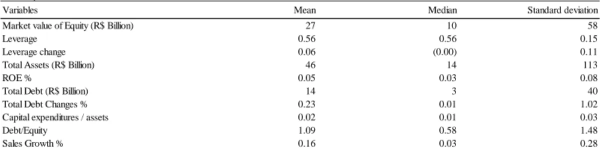
Table 1 reports the summary statistics of the level and change in leverage ratio of the firms in the sample. The average firm has a leverage ratio of 0.56. As mentioned before, leverage change is defined as the change in book leverage from the previous quarter. The average leverage change is 0.06 which is justified by the fact that the change can either be positive or negative which results in a net effect close to zero, on average. Nonetheless, the quarterly standard deviation is 11%. Total debt change is much lower than leverage changes, with a value of an average of 0.23%. The sales growth is on average 0.16% and the ROE 0.05%. Finally, the average debt-to-equity ratio (financial ratio that indicates the relative proportion of the entity’s equity and debt used to finance an entity’s assets) is close to 1 (1.09) meaning that, the companies in the sample, according to the literature, have an optimal debt-to-equity ratio, even though it varies according to each industry. For example, US companies show the average debt-to-equity ratio is 1.5.
IV - Empirical analysis
Leverage changes and stock returns
In this section I provide evidence on how changes in a firm’s leverage level affect its stock price. Various portfolios are constructed on the basis of the change in the leverage ratio, whereby firms are sorted in this analysis from the highest change to the lowest change. Thus, for each quarter, two portfolios are constructed: portfolio 1 comprising of firms with positive changes and
portfolio 2 consisting of firms with negative changes resulting in 67 portfolios with positive changes in leverage ratio and 67 portfolios with negative changes in leverage ratio. Note that each portfolio has different component stocks in every quarter since the sorting is based on the change in the leverage ratio. Next, the equally weighted quarterly returns for each portfolio is calculated during both the current quarter and the next quarter of leverage change. Table 2 presents the results for the equally weighted portfolio returns for portfolios sorted by the current quarter leverage change. The first column shows the results for the portfolios with positive leverage change. The second column refers to the portfolios with negative changes in the leverage ratio. We find that the average portfolio quarterly returns increase with both positive and negative changes in the leverage levels by 5.6% and 5.9%, respectively.
Given that the change in leverage may occur at any time of a quarter and is often reported during the next quarter, the current quarter returns may not capture all the information, and ultimately does not measure the impact of the leverage change. Thus, the relationship between changes in leverage and the next quarter stock returns are examined. Note that, there are no values for 2000 and last quarter of 2016 since some observations had to be taken off the sample to pursue this analysis. The results are reported in table 2 (columns 3 and 4). Again, I find that for both, positive and negative changes’ portfolios, the average portfolio return increases by 6.1% and 5.8%, respectively.
Table 1
Summary statistics
Variables Mean Median Standard deviation
Market value of Equity (R$ Billion) 27 10 58
Leverage 0.56 0.56 0.15
Leverage change 0.06 (0.00) 0.11
Total Assets (R$ Billion) 46 14 113
ROE % 0.05 0.03 0.08
Total Debt (R$ Billion) 14 3 40
Total Debt Changes % 0.23 0.01 1.02
Capital expenditures / assets 0.02 0.01 0.03
Debt/Equity 1.09 0.58 1.48
Sales Growth % 0.16 0.03 0.28
The sample consists of all nonfinancial firms that have positive book value of equity and non-negative book value of total liabilities. Sample was made available through Economática and Thomson Reuters for the period of 2000 to 2016. At the end of each quarter, it was calculated the percentual change in leverage ratio. Leverage is defined as the ratio between the book value of total liabilities and the book value of total assets
It is possible that the observed positive relationship between leverage changes and stock returns are associated with unexpected increases recorded (one characteristic of emerging markets is high volatility due to economic or political reasons) in some companies due to the impact of volatile currencies that are more common in emerging markets. This is particularly true for Brazil,
Table 2
Equal-weighted quarterly stock returns of Portfolios sorted by quarterly leverage changes
Date Positive changes' portfolio Negative changes' portfolio Positive changes' portfolio Negative changes'
portfolio Mean (%) Median (%)
2T2000 1 6.1% 1.5% - - 0.55 -3T2000 2 5.4% 6.7% - - (1.89) (0.69) 4T2000 3 (2.4%) (3.0%) - - (3.09) (1.72) 1T2001 4 9.8% 1.8% (7.1%) 10.0% (4.69) (2.12) 2T2001 5 (6.5%) 5.8% (16.5%) (20.2%) (2.55) (2.53) 3T2001 6 (18.8%) (6.7%) 30.6% 13.7% (4.77) (2.19) 4T2001 7 23.2% 33.7% 14.9% 14.7% (2.19) (3.19) 1T2002 8 14.9% 14.7% (4.9%) (4.5%) (0.49) (1.54) 2T2002 9 (5.3%) 0.3% (20.1%) (12.9%) (1.06) (1.17) 3T2002 10 (17.9%) (33.5%) 29.2% 14.1% 2.93 (1.28) 4T2002 11 33.8% 24.9% (10.9%) 3.7% (1.27) (1.24) 1T2003 12 (10.9%) 3.7% 18.8% 20.4% (1.69) (1.35) 2T2003 13 16.4% 20.6% 36.3% 27.3% (3.53) (2.77) 3T2003 14 32.5% 25.0% 60.1% 42.0% (1.15) (0.84) 4T2003 15 51.7% 41.0% (11.1%) 10.6% 1.41 0.97 1T2004 16 (11.1%) 10.6% (13.2%) 0.6% (2.87) (2.03) 2T2004 17 (2.5%) (2.5%) 20.9% 22.4% 0.36 -3T2004 18 26.2% 19.7% 11.7% 12.8% (0.75) -4T2004 19 11.8% 13.7% (1.2%) 1.7% 3.88 2.63 1T2005 20 (1.2%) 1.7% (4.1%) (7.2%) (3.81) (3.49) 2T2005 21 (0.8%) (10.5%) 23.7% 28.5% (0.58) -3T2005 22 28.1% 21.5% 13.9% 10.3% (0.81) (1.15) 4T2005 23 10.0% 19.0% 20.4% 22.1% (0.71) (0.60) 1T2006 24 20.4% 22.1% (5.0%) (3.3%) (2.78) (1.99) 2T2006 25 (4.2%) (3.1%) 2.6% 3.3% (0.91) (0.86) 3T2006 26 3.0% 2.8% 20.1% 17.3% (3.14) (2.89) 4T2006 27 19.8% 14.9% 10.1% 1.9% (0.65) (0.50) 1T2007 28 10.1% 1.9% 13.0% 20.5% (1.08) (0.78) 2T2007 29 15.5% 20.0% (0.7%) 2.6% 1.83 1.32 3T2007 30 (2.0%) 4.4% (4.9%) 2.3% 0.34 0.63 4T2007 31 (0.2%) (4.7%) (4.7%) 1.0% (0.85) -1T2008 32 (4.7%) 1.0% 1.8% 9.4% (0.20) (0.15) 2T2008 33 2.7% 9.5% (16.6%) (21.0%) (0.72) (1.37) 3T2008 34 (20.3%) (17.6%) (20.1%) (14.8%) (2.11) -4T2008 35 (17.7%) (27.6%) 13.1% 4.2% 2.44 1.85 1T2009 36 13.1% 4.2% 39.7% 28.7% 7.66 8.45 2T2009 37 32.4% 32.0% 23.0% 18.0% 0.41 (0.12) 3T2009 38 16.7% 20.3% 15.3% 14.6% (4.93) (3.22) 4T2009 39 14.4% 15.6% (1.0%) (1.5%) (2.15) (0.55) 1T2010 40 (1.0%) (1.5%) (0.4%) (3.2%) (0.23) -2T2010 41 (1.4%) (2.9%) 9.1% 10.0% (1.25) (0.59) 3T2010 42 7.1% 11.9% 4.0% 4.9% 1.40 0.29 4T2010 43 2.3% 8.8% 0.2% 0.8% (2.41) (0.53) 1T2011 44 0.2% 0.8% (5.2%) (3.9%) (0.46) (0.33) 2T2011 45 (6.9%) (2.3%) (12.2%) (10.8%) 1.14 1.73 3T2011 46 (12.7%) (7.9%) 11.7% 8.5% 0.59 0.24 4T2011 47 10.8% 10.9% 19.6% 18.4% 0.19 (0.20) 1T2012 48 19.6% 18.4% (3.4%) (3.7%) 1.13 0.72 2T2012 49 (7.5%) 4.5% 11.5% 7.2% 3.52 2.17 3T2012 50 11.2% 8.8% 5.7% 6.0% (0.37) 0.03 4T2012 51 0.8% 14.4% (2.6%) 0.8% 3.06 0.10 1T2013 52 (2.6%) 0.8% (5.2%) (8.5%) 2.38 (0.90) 2T2013 53 (9.7%) (4.7%) 13.5% 7.2% (1.10) (2.42) 3T2013 54 11.7% 10.3% (1.5%) 6.5% 3.16 1.02 4T2013 55 3.1% 2.9% (1.8%) (2.2%) 4.16 0.87 1T2014 56 (1.8%) (2.2%) 9.8% 4.4% 6.85 3.61 2T2014 57 8.4% 4.9% 0.5% 0.5% 5.77 2.07 3T2014 58 2.9% (3.2%) (6.9%) 0.0% 4.27 3.52 4T2014 59 (4.1%) (4.8%) 1.6% 2.5% 12.57 5.21 1T2015 60 1.6% 2.5% 5.5% (2.2%) 2.97 1.90 2T2015 61 3.9% 1.7% (20.1%) (10.8%) 3.97 2.59 3T2015 62 (15.2%) (15.4%) (1.2%) 4.0% 8.42 1.55 4T2015 63 (0.4%) 2.1% 26.8% 15.6% 3.23 1.15 1T2016 64 26.8% 15.6% 21.5% 6.0% 1.36 0.68 2T2016 65 8.6% 10.0% 14.3% 18.6% 3.51 2.24 3T2016 66 22.2% 11.9% 9.2% (3.2%) 1.62 1.23 4T2016 67 4.9% (1.4%) - - 2.56 3.29
Portfolios of current quarter returns sorted by current quarter leverage change
Portfolios of next-quarter returns sorted by current quarter leverage change
Leverage change current quarter(%)
Leverage change Portfolios
The sample consists of all nonfinancial firms that have positive book value of equity and non-negative book value of total liabilities. Sample was made available through Economática and Reuters for the period of 2000 to 2016. At the end of each quarter, it was calculated the percentual change in leverage ratio. Then I sort the sample into two portfolios per quarter by the leverage change in the current quarter. The number of stocks per portfolio is dependent on the number of firms that have changed their leverage ratio in the quarter in analysis.
due to its relationship with the US dollar, which is caused by the country’s high dependence on oil and food imports and Brazil’s economic and political instability. Thus, I examine whether popular asset pricing models can explain this positive relationship. Three models were considered: The Capital Asset Pricing Model (CAPM), the Fama-French (1993) three-factor model, and the Carhart (1997) four-factor model (three-factor plus the momentum factor) for the vector in table 2 with all the returns from each portfolio (positive and negative leverage changes’ portfolios). I run the following regression:
𝑅𝑖,𝑡− r𝑓,𝑡 = α + β’𝑖F𝑡+ ɛ𝑖,𝑡 (for i = 1 to 2)
Where Rit are the quarterly portfolio returns vector, and rft is the risk free rate measured by the three month US T-Bill yield. Ft is a vector of factor returns including the market excess return (my first approach uses global market excess return and 3 months US T-Bill not adjusted to inflation), returns of the Fama-French factor’s including size: SMB, book-to-market: HML, and the momentum factor: UMD. The return series of these factors and the three month US T-Bill yield were obtained from the Kenneth French’s website. Note that the model was tested for heteroscedasticity, autocorrelation and normality of residuals and a conclusion was drawn for the negative changes’ portfolio, the residuals are heteroscedastic meaning that the coefficients are not efficient which would lead to incorrect inference and significance conclusions. Therefore, I use the estimated model corrected for heteroscedasticity on which all OLS conditions are fulfilled. Regarding the positive changes’ portfolios, there were no problems regarding the residuals of the coefficients, since I have not rejected the null hypothesis for all the three tests mentioned above. For both, I used the Breusch-Pagan-Godfrey’s test for homoscedasticity, the Breusch-Godfrey test for autocorrelation and tested the normality of residuals through Skewness, Kurtosis and Jarque-Bera.
If the factors mentioned above can explain the excess return in both, positive and negative changes’ portfolios, the alphas are expected to be similar. Note that we got a high and identical alpha for both regressions (4.6%), and found that they are statistically significant. An additional analysis was performed in order to check if different results could be obtained with regards to the variables’ significance power and alpha values that explain the positive relation between changes in leverage and stock returns. Thus, in my second approach, Ibovespa excess return is used instead of the global market excess return and the US T-Bill yield is adjusted for inflation instead of the US T-Bill yield. Note that in order to use the US T-Bill I need to adjust the rate for the inherent risks of the Brazilian market. For that, the US T-Bill was multiplied and divided by “1+ inflation” for each trimester of Brazil and US, respectively, as shown below. The results of the significance of the independent variables were identical but a lower alpha (2.5% and 3.0% for positive changes and negative changes’ portfolios, respectively) was found, as shown in table 5.
((1 + 𝑈𝑆𝐷 𝑇𝐵𝑖𝑙𝑙 𝑦𝑖𝑒𝑙𝑑 𝑖𝑛 𝑈𝑆𝐷)(1 4)⁄ ×
(1 + 𝐼𝑛𝑓𝑙𝑎𝑡𝑖𝑜𝑛 𝐵𝑅𝐿)(1 4⁄ )
(1 + 𝐼𝑛𝑓𝑙𝑎𝑡𝑖𝑜𝑛 𝑈𝑆𝐷)(1 4)⁄ ) − 1
Table 3 displays the results of both regressions (positive and negative changes portfolios) using global market excess return and the risk free (not adjusted for inflation). The first four columns report the results for the portfolios with positive changes and latter four columns report the results for the portfolios with negative changes in leverage ratio. They reveal that the capital asset pricing model (CAPM) is significant to explain the positive effect of leverage on stock returns. On the other hand, it is concluded that the other factors (Fama-French and Carhart (1997)) are not significant in explaining the positive relationship between returns and changes in leverage ratio. Please note that the alphas are practically identical in both, positive and negative changes’ portfolios, meaning that other market risks (not contemplated in the previous models) explain the difference in returns (returns of the two portfolios can be different due to other market risks which
are not captured by the beta of the CAPM). Thus, after controlling for the risks, the difference in return is expected to be close to zero.
An additional analysis was made defining leverage as the percentage change of the debt level with identical results. The impact of this is that relative changes in the amount of debt are not controlled for, which may result in a biased analysis. Therefore, in this paper, leverage is used as the ratio between total book value of liabilities divided by the total book value of assets.
In addition, I perform the same analysis but with the impact in next quarter returns of current quarter changes in leverage. The results are listed in table 4.
As the results from the regression using next quarter returns of current quarter changes in leverage were not statistically significant, I will proceed with the analysis using current quarter returns with current quarter leverage changes.
Table 3
Quarterly stock returns of portfolios sorted by quarterly leverage changes Coefficients
Positive changes
portfolio Estimate Standard
error
t value Pr(>|t|) Negative changes
portfolio Estimate Standard
error
t value Pr(>|t|)
Intercept 0.04673 0.01449 3.225 0.00201 Intercept 0.04592 0.01167 3.933 0.000214
Market excess return 2.6298 0.50404 5.217 2.22E-06 Market excess return 3.00239 0.40605 7.394 4.46E-10
SMB 0.97595 1.36802 0.713 0.47827 SMB 1.53285 1.10207 1.391 0.169231
HML 0.31881 0.79239 0.402 0.68882 HML 0.4894 0.63834 0.767 0.446186
WML -1.13167 0.56281 -2.011 0.04871 WML -0.54817 0.45339 -1.209 0.231241
The sample consists of all nonfinancial firms that have positive book value of equity and non-negative book value of total liabilities. Sample was made available through Economática and Reuters for the period of 2000 to 2016. At the end of each quarter, it was calculated the percentual change in leverage ratio. Then it was sorted the sample into two portfolios per quarter by the leverage change in the current quarter. The number of stocks per portfolio is dependent on the number of firms that have changed their leverage ratio in the quarter in analysis.
Table 4
Quarterly stock returns of portfolios sorted by quarterly leverage changes Coefficients
Positive changes
portfolio Estimate Standard
error
t value Pr(>|t|) Negative changes
portfolio Estimate Standard
error
t value Pr(>|t|)
Intercept 0.06357 0.0221 2.877 0.00561 Intercept 0.05931 0.01711 3.467 0.000999
Market excess return -0.34237 0.76694 -0.446 0.65696 Market excess return -0.46137 0.59377 -0.777 0.440309
SMB 0.92442 2.22447 0.416 0.67926 SMB 0.47505 1.72219 0.276 0.783653
HML -0.05326 1.60703 -0.033 0.97368 HML 0.03877 1.24417 0.031 0.975248
WML -0.86685 0.94429 -0.918 0.36243 WML -0.26172 0.73108 -0.358 0.721653
The sample consists of all nonfinancial firms that have positive book value of equity and non-negative book value of total liabilities. Sample was made available through Economática and Reuters for the period of 2000 to 2016. At the end of each quarter, it was calculated the percentual change in leverage ratio. Then it was sorted the sample into two portfolios per quarter by the leverage change in the current quarter. The number of stocks per portfolio is dependent on the number of firms that have changed their leverage ratio in the quarter in analysis.
The high and positive alpha (table 3) forced me to change some variables, as mentioned before, which resulted in a lower alpha as presented below in table 5. Thus, it is fair to say that these asset-pricing models cannot fully explain the positive effect of leverage changes on stock returns since we test the hypothesis that the “alpha” is equal to zero and we reject this null hypothesis when using all three asset-pricing models. Please note that I first tested the hypothesis that alpha is equal to zero for the CAPM alone and concluded that there is a positive and significant alpha. After that, I tested the alpha in the 3-factor model and noticed a decrease in the alpha but it was still positive and significant. Lastly, I tested in the 4-factor model where the result was quite odd since the alpha increased, even though it is still significant, the R2 was roughly the same (82%% and 78% for positive and negative changes portfolios, respectively). This led to the conclusion that the momentum factor does not add significance to the model and, therefore, was excluded from the event date analysis. The alpha values from both portfolios are presented in table 6 below. For the two portfolios presented below (table 6) an increase in the alphas trends as the leverage ratio change goes from positive to negative is observable. In the CAPM model, the alpha equals to 3% for the positive changes portfolio and 3.6% for the negative changes portfolio, with a difference of 0.6%. Note that, both alphas are statistically significant at the 1% level. It is important to refer that the difference in both alphas is very similar to the difference in the portfolios returns (0.3% (average positive portfolio return 5.6%; average negative portfolio return 5.9%)) suggesting that the positive effect of leverage changes on stock returns cannot be explained by the market factor. As more factors are added to the regression models (three factor and four factor models) the results are roughly the same. For both models, I still find an increase in the alphas trends as the leverage ratio change goes from positive to negative. The difference in alphas between both portfolios is equal to 0.6% in the three-factor model and equal to roughly 0.5% in the four-factor model, with both alphas statistically significant at the 1% level.
By individually testing the null hypothesis of alpha equal to zero, we reject it for the three asset pricing models, and conclude that there are abnormal returns; I use another methodology in order to quantify the short-term abnormal returns, the Event Study Methodology. It is important to refer that it is possible that the change in leverage may come from a decision a firm makes in the short term.
Event study
Although some of the above factors are not statistically significant to explain the positive relationship between changes in leverage ratio and the current and next quarter stock returns, a firm’s capital structure choice may depend on other characteristics not captured by these factors. It is possible that the positive relationship between changes in the leverage ratio and stock returns is explained by other firm characteristics, together with the above factors. Moreover, it is possible that it is explained by decisions the firm makes regarding ongoing positive NPV projects and how to finance the projects in the short term. Thus, in order to individually analyze the impact of changes in the leverage ratio and to quantify the short-term abnormal stock returns (difference between
Table 5
Quarterly stock returns of portfolios sorted by quarterly leverage changes Coefficients
Positive changes portfolio Estimate Standard error
t value Pr(>|t|) Negative changes portfolio Estimate Standard error
t value Pr(>|t|)
Intercept 0.025369 0.008334 3.043992 0.0034 Intercept 0.030047 0.008422 3.567693 0.0007
Market excess return (Ibovespa) 0.917167 0.062084 14.77296 0.0000 Market excess return (Ibovespa) 0.820444 0.06274 13.07697 0.0000
SMB 0.759266 0.761824 0.996643 0.3228 SMB 1.760221 0.769867 2.286398 0.0257
HML 0.826792 0.44683 1.850348 0.069 HML 0.743231 0.451548 1.645963 0.1048
WML -0.220521 0.325073 -0.678374 0.5001 WML 0.006891 0.328505 0.020978 0.9833
The sample consists of all nonfinancial firms that have positive book value of equity and non-negative book value of total liabilities. Sample was made available through Economática and Reuters for the period of 2000 to 2016. At the end of each quarter, it was calculated the percentual change in leverage ratio. Then it was sorted the sample into two portfolios per quarter by the leverage change in the current quarter. The number of stocks per portfolio is dependent on the number of firms that have changed their leverage ratio in the quarter in analysis.
Table 6
Risk-adjusted returns of portfolios sorted by leverage changes Coefficients Positive changes portfolio Alpha Estimate Standard error t value Pr(>|t|) Adjusted R2 Negative changes portfolio Aplha Estimate Standard error t value Pr(>|t|) Adjusted R2 CAPM 0.030073 0.007643 3.93486 0.0002 0.8103 CAPM 0.036172 0.007844 4.611672 0.0000 0.7660
Three Factor Model 0.02385 0.007993 2.983791 0.0040 0.8187 Three Factor Model 0.030095 0.008048 3.739591 0.0004 0.7848
Four Factor Model 0.025369 0.008334 3.043992 0.0034 0.8171 Four Factor Model 0.030047 0.008422 3.567693 0.0007 0.7813
The sample consists of all nonfinancial firms that have positive book value of equity and non-negative book value of total liabilities. Sample was made available through Economática and Reuters for the period of 2000 to 2016. At the end of each quarter, it was calculated the percentual change in leverage ratio. Then it was sorted the sample into two portfolios per quarter by the leverage change in the current quarter. The number of stocks per portfolio is dependent on the number of firms that have changed their leverage ratio in the quarter in analysis.
realized and expected returns), I conduct the event study methodology having as an event date, the quarter with the highest leverage ratio during the complete period (please refer to the diagram below). Note that this analysis was only performed for 27 companies since they were the ones with sufficient available data to estimate the models including data of two quarters before and after the event date of stock returns.
This paper assumes that the estimation window will be from 2000 until the maximum leverage ratio is verified, and 2 quarters for the event window (-2, 2) for each of the firms in the sample, fulfilling the conditions mentioned above. For this purpose, this study uses the capital asset pricing model (CAPM), the Fama French 3-factors and the stock returns of the chosen companies to estimate the models to calculate the expected returns which are further compared with the actual stock returns. The return of the Ibovespa index was obtained from Economática, Fama-French 3 factors model and the three month US T-Bill were obtained from the Kenneth French’s website (the US T-Bill is farther adjusted to inflation). An additional model is computed with additional independent variables in order to control for other factors. I include the leverage ratio change and leverage ratio in order to control for the time-invariant effect, which was reported by Lemmon et al (2008). I also include the previous quarter ROE to control for the effect of earnings on stock
-2 0 2 Event study 0: Maximum leverage change from 1T2000 to 4T2016 T2: Ending of event window T1: Beginning of event window T0: Beginning of estimation period X
Note: X varies according to each company analyzed since available data varies from company to company.
returns and Debt to Equity ratio to control for market imperfections (Bhandari 1988). The following regression is estimated for each company.
𝑅𝑖,𝑡− r𝑓,𝑡 = α + β’𝑖F𝑡+ β’𝑐𝑜𝑛𝑡𝑟𝑜𝑙,𝑡(control vector) + ɛ𝑖,𝑡
Whereby, Rit is the quarterly returns of each company, and rft is the risk free rate measured by the three month US Treasury Bill yield adjusted to inflation. Ft is a vector of factor returns including the market excess return) and returns of the Fama-French factor’s including size: SMB and book-to-market: HML.
This data was used to build the event study and calculate the existence of abnormal returns (AR) and cumulative abnormal returns (CAR) during the event window. Please note that as abnormal returns were obtained in the previous analysis (please see table 6), it is expected that the stock returns forecasted in the models do not fully capture the actual stock returns giving rise to abnormal returns (alphas).
The event window period was assumed to be 2 quarters before and after the maximum amount of debt recorded in the sample once this is the period where impact of changes in the leverage ratio is expected to be reflected in the stock returns since, as it was said before, changes are often reported during the next quarter. In addition, the CAPM model is used to verify the results obtained in the previous regression (please see table 5), which found that the CAPM model is significant to explain the positive portfolio returns when changes in leverage ratio occur. Regarding the three-factor model, I want to test if the other variables used in the previous analysis (only SMB variable is statistically significant to explain positive effect of leverage on stock returns) are significant to explain the relationship between stock returns and leverage change, individually for each company in a specific period. Thus, we forecast the expected return of the stock and compare it with the actual return in order to find the existence of abnormal returns. Please note that cumulative
abnormal returns have also been calculated to measure the returns over the event window. To calculate both, the abnormal return and the cumulative abnormal return I use the following formulas:
𝐴𝑅𝑖,𝑡 = 𝑅𝑖,𝑡− 𝐸(𝑅𝑖,𝑡) CARi,t = ∑𝑇𝑡=1𝐴𝑅𝑖,𝑡
As a way of measuring the veracity of the obtained results, a standard t-test was used to both abnormal and cumulative abnormal returns. Moreover, each regression is tested regarding heteroskedasticity, autocorrelation and normality of the residuals. When a problem regarding the residuals is found, the estimated model is corrected for it, being the analysis proceeded with the correct model. To pursue the study, I divided the companies into two portfolios according to the average leverage ratio. Hence, companies with leverage ratio higher than the average go to portfolio 1 and companies with leverage ratio lower than the average go to portfolio 2 (average leverage ratio presented in table 1). The results obtained clearly corroborate with the previous analysis since it was obtained positive values for both, abnormal returns and cumulative abnormal ones when a firm reaches their maximum change of leverage ratio. Note that, the abnormal and cumulative abnormal returns were found significant.
According to capital structure literature, many other variables were identified as variables that may affect a firms’ choice regarding the leverage ratio. Table 7 reports the time series averages of the estimated regression coefficients and, below every coefficient, the corresponding t-statistics. Regression one only includes the Ibovespa excess return (CAPM) and regression two includes the Fama and French 3 factors model variables. In regression 3, I include all other control variables. We found positive alphas for the first two regressions on which we verify a decrease from the CAPM Model to the Fama and French 3 factors meaning that as we add the variables to control for size and value, the alpha decreases. Regression 3 presents a different result since as I add more
control variables, the alpha decreases to a negative value even though they are not significant. This led me to conclude that some control variables are helping to control for the alpha significant since the adjusted R2 remains practically identical from model 2 to model 3. Moreover, the Ibovespa excess return coefficient is also practically identical and significant which confirm the results obtained in the previous regressions. In regression 3, the average coefficient for the leverage change is positive being consistent with the previous analysis. Regarding ROE from previous quarter, the average coefficient is 0,26 meaning that for an increase of 1 basis point in the ROE, it has a positive impact of 0,26 basis points on stock returns. On the other hand, Debt to Equity ratio has an average coefficient of (-0,15) meaning that for an increase of 1 basis point in the Debt to Equity ratio, it has a negative impact on stock returns.
Table 7
Time series return regression
Independent variables and statistics
Model 1 - CAPM Model 2 - FF 3
factor
Model 3 - Model 2 with control variables
R2 0,32 0,34 0,34
Alpha 0.032 0.027 (0.045)
(1.12) (0.97) (0.16)
Ibovespa excess return 0.84 0.82 0.76
(4.55) (4.30) (4.16) SMB 1.79 1.43 (0.67) (0.21) HML 0.18 0.29 (0.04) (0.11) Leverege 0.50 (0.14) Leverege change 0.04 0.34 ROE 0.26 (-0.119)
Debt to Equity ratio (0.15)
(-0.457)
N 27 27 27
Dependent variable - quarterly stock excess return (%)
This table reports estimation results for cross sectional regressions. In each quarter we run the cross sectional regressions for all available firms assuming variables are constant. The dependent variable is the stock return in each quarter. The independent variables include the market excess return (CAPM), Fama French 3 factors, leverage change and ROE at the most recent fiscal quarter end and the leverage level at the beginning of the most recent quarter. ROE equals to net income divided by the book value of equity. I report the average coefficients of all regressions and report their t-statistics in parentheses.
V - Conclusion
In this paper, I document that the average portfolio quarterly returns increase with both positive and negative changes in the leverage levels. I examine whether popular asset pricing models can explain this positive relationship and conclude that the CAPM model is significant to explain the positive relationship but the Fama and French 3 factor model and Carhart 4 factor model are not significant. In my first approach (global market excess return and USD Treasury-Bill not adjusted to inflation were used) I found an identical alpha on both portfolios meaning that the difference in return is explained by other market risks, not contemplated in the previous models. In my second approach (Ibovespa excess return and USD Treasury-Bill adjusted to inflation are used), I find lower alphas but still significant using all three asset pricing models. Thus, I conclude that that these asset-pricing models cannot fully explain the positive effect of leverage changes on stock returns. Through the employment of the Event study methodology, to quantify the short-term abnormal returns, I find the existence of abnormal returns since I reject the null hypothesis that abnormal return equals to zero. Finally, I run time series regressions for each company individually using CAPM model and Fama French 3 factor and add other control variables and conclude that only the market excess return is significant which corroborates with the previous analysis.
VI - References
Acheampong, Prince, Evans Agalega, and Albert Kwabena Shibu. 2013. "The Effect of Financial Leverage and Market Size on Stock Returns on the Ghana Stock Exchange: Evidence from Selected Stocks in the Manufacturing Sector." International Journal of Financial
Research 125-134.
Bhandari, Laxmi Chand. 1988. "Debt/Equity Ratio and Expected Common Stock Returns: Empirical Evidence." The Journal of Finance 507-528.
Cai, Jie, and Zhe Zhang. 2011. "Leverage change, debt overhang, and stock prices." Journal of
Corporate Finance 391-402.
Drobetz, Wolfgang, and Pascal Pensa. n.d. Capital Structure and stock returns: The European
Gomes, Joao F., and Lukas Schmid. 2010. "Levered Returns." The Journal of Finance VOL. LXV, NO.2.
Goyal, Vidhan K., and Murray Z. Frank. 2009. "Capital Structure Decisions: Which Factors Are Reliably Important." Financial Management 1-37.
Hatfield, Gay B., Louis T.W. Cheng, and Wallace N. Davidson. 1994. "The Determination of Optimal Capital Structure: The Effect of Firm and Industry Debt Rations on Market Value." Journal of Financial And Strategic Decisions Volume 7 Number 3.
Korteweg, Arthur. 2004. Financial Leverage and Epected Stock Returns: Evidence from Pure
Exchange Offers. University of Chicago Graduate School of Business.
Lau, Wei-Theng, Siong-Hook Law, and Annuar Md Nassir. 2016. "Debt Maturity and Stock Returns: An Inter-Sectoral Comparison of Malaysian Firms." Asian Academy of
Management Journal of Accounting and Finance (Asian Academy of Management
Journal of Accounting and Finance) 37-63.
Lyle, Nicholas. 2017. Debt/Equity Ratio and Asset Pricing Analysis. Utah State University. Muradoglu, Gulnur, and Sheeja Sivaprasad. 2008. An Empirical Test on Leverage and Stock
Returns. Cass Business School.
Obreja, Julian. 2013. "Book-to-Market Equity, Financial Leverage, and the Cross-Section of Stock Returns." Oxford Journals 1146-1189.
Prescott, Edward C., and Ellen R. McGrattan. 2003. "Average Debt and Equity Returns." The
American Economic Review 392-397.
Sibindi, Athenia Bongani. 2016. Determinants of Capital Structure: A Literature Review. Risk Governance & Control: Financial Markets & Institutions.
Tahmoorespour, Reza, Mina Ali-Abbar, and Elias Randjbaran. 2015. "The Impact of Capital Structure on Stock Returns: Internatinal Evidence." Hyperion Economic Journal 56-78. Titman, Sheridan, Tim Opler, and Armen Hovakimian. 2001. "The Debt-Equity Choice." The
Journal of Financial and Quantitative Analysis 1-24.