Data confession in the portuguese EDM

DOCUMENTOS DE TRABALHO

WORKING PAPERS

ECONOMIA

ECONOMICS

Nº 09/2008

DATA CONFESSION IN THE PORTUGUESE EDM REGION

Leonardo Costa

DATA CONFESSION IN THE PORTUGUESE EDM REGION

Leonardo Costa (1₎

(1_{) Portuguese Catholic University, Faculty of Economics and Management, Porto, Portugal – leocosta@porto.ucp.pt} KEYWORDS

water, agricultural economics, elasticities, positive mathematical programming, maximum entropy.

ABSTRACT

A dual profit model is used to characterize the Entre Douro e Minho (EDM) region agriculture. The data comes from budgets for twelve representative farms. Positive Mathematical Programming (PMP) is applied. First, shadow prices of fixed inputs are obtained for each farm from a linear program (LP) forcing base year (1994) net output and fixed input allocations. Second, the Maximum Entropy (ME) technique is used to recover the restricted profit functions. The model purely reproduces observed net output and fixed input data. A short run profit function is derived for the region from aggregation of the model. The corresponding long run profit function is also derived.

The profit model reveals an inelastic response to prices in the short run, and a more elastic response in the long run. Nitrogen and water appear as complements. The inelasticity of nitrogen response to its own price precludes taxing nitrogen to control its use. In contrast, pricing water is an effective strategy, not only to control water use but also nitrogen use. The Water Framework Directive (WFD) recommends both strategies.

INTRODUCTION

This paper illustrates how Positive Mathematical Programming (PMP) and Maximum Entropy (ME) techniques can be used in the process of information recovery (data confession) when data are very scarce. A dual profit model characterizing the Entre Douro e Minho (EDM) region agriculture is recovered. The data are the budgets of twelve representative farms for the region (Monke et al., 1998).1 PMP is applied. First, shadow prices of fixed inputs are obtained for each farm from a linear program (LP) forcing base year (1994) net output2 and fixed input allocations (Howitt, 1995a,b; Paris and Howitt, 1998). Second, the Maximum Entropy (ME) technique is used to recover the restricted profit functions (Golan, Judge, and Miller, 1996; Paris and Howitt, 1998). The model purely reproduces observed net output and fixed input data. A short run profit function is derived for the region from aggregation of the model. The corresponding long run profit function is also derived.3

1 _{The data has been aggregated in each representative farm to distinguish two outputs, two variable inputs, and four fixed}

inputs. The outputs are capmsc and caplsc, respectively the farms’ Common Agricultural Policy (CAP) most supported and less supported commodities. The output capmsc includes corn, milk, beef, and lamb. The output caplsc includes potatoes, winter and summer vegetables, wine, and apples. The two variable inputs are nitrogen and energy. Energy includes electricity, gas, oil, fertilizer other than nitrogen, and pesticide. The four fixed inputs are water, land, labor, and capital. Labor includes family and hired labor. Capital includes mainly the annual cost of equipment and livestock. Water is treated as a fixed input because most of the water comes from private small springs and wells. There is no formal agricultural water market (or water price) in the EDM. Water quantities are measured in physical units (10E+4 cubic meters). All other inputs and outputs are measured in 1994 prices Differences in the composition of outputs and inputs in quality and in CAP support are reflected in the quantity variables (Cox and Wohlgenant, 1986; Oude Lansink and Thijssen, 1998). The 1994 base year prices are a simple average of 1993, 1994, and 1995 prices. There is no price variability in the data except for shadow prices of fixed inputs obtained in the LP first stage of PMP.

2 _{Net output can be an output or a variable input.}

3 _{The properties of the restricted and the unrestricted profit functions are related by the virtual pricing approach (Rothbarth,}

1941; Neary and Roberts, 1980; Squires, 1987, 1994; Quiroga et al., 1992, 1995). Virtual prices lead unrestricted farmers to behave as if they were facing restrictions. But virtual prices also lead restricted farmers to behave as if they were not facing restrictions. Thus, the short run shadow prices of fixed inputs might be regarded as virtual prices. A link can be established between the parameters of the short run restricted profit function and the long run (unrestricted) profit function:

___________________________________________________________________________ The profit model uses the normalized quadratic restricted profit function. This function was preferred to the translog because it allows for zero levels of outputs and inputs, and has the property that local convexity implies global convexity. The coefficients of the Hessian matrix are constant, allowing simple derivation of the long run unrestricted profit function (Lau, 1976). The function has some drawbacks. The monotonicity condition is not necessarily globally satisfied. The functional form imposes quasi-homotheticity and separability restrictions (Lopez, 1985). Estimation results are not invariant to the choice of numeraire (Oude Lansink and Thijssen, 1998).4

The mathematical expression of the normalized quadratic restricted profit function is the following:

∑∑

∑∑

∑∑

∑

∑

− = = = = − = − = = − =

+

+

+

+

+

=

Π

1 1 1 1 1 1 1 1 1 1 1 1

2

1

2

1

)

,

(

m k v r r k kr v r s v s r rs m k m l l k kl v r r r m k k k

z

p

e

z

z

d

p

p

c

z

b

p

a

u

Z

p

(1)

where

∏

(

p

,

Z

)

are profits, p are normalized net output prices, and

Z

are fixed input quantities. Net output prices are normalized by the price of the mth net output, so

m k k

P

P

p

=

.5

PROFIT MODEL RECOVERY

In the profit model context, PMP has two stages. Let i

(

,

i

)

Z

p

Π

be farm i’s restricted profit function, p a set of

k

=

1

,...,

(

m

−

1

)

net output normalized prices, and

Z

i a set of

v

=

1

,...,

r

fixed inputs. The restricted profit function yields

k

=

1

,...,

(

m

−

1

)

net output supply equations,

)

,

(

i

i k

p

Z

Y

, and

v

=

1

,...,

r

shadow price equations,

SH

_ri

(

p

,

Z

i

)

. In the first stage of PMP, a linear programming (LP) model recovers fixed input shadow prices for each representative farm. In the second stage, the Maximum Entropy (ME) technique is used to recover net output supply and shadow price equations, consistent with a quadratic profit function. The ME problem is formulated and solved as a pure inverse problem (Golan, Judge, and Miller, 1996). The model reproduces base year data consistent with economic theory.

The LP model for each farm takes the following specification in matrix notation:

i Z Y

pY

Max

i i

(2)

ST

0

≤

i

AY

(3)

b

BZ

i

≤

(4)

{

p

Z

wZ

}

Max

w

p

Z

Π

−

=

Π

(

,

)

(

,

)

, where

Π

(

p

,

w

)

is the long run (unrestricted) profit function,

Π

(

p

,

Z

)

is the short run restricted profit function, p the prices of outputs,

Z

the fixed inputs, and w the virtual prices of fixed inputs.

4 _{Homogeneity of the normalized quadratic functional form requires a net output for asymmetrical treatment.}

5 _{Sufficient conditions to ensure duality are that profit is a non-negative real valued function, non-decreasing in output price and}

non-increasing in input price, non-decreasing in

Z

for every fixed p, linear homogeneous in p and

Z

, convex and continuous in p for every fixed

Z

, and concave and continuous in

Z

for every fixed

p

.

(

Y

)

i i

Y

Y

≤

1

+

ε

(5)

(

Z

)

i i

Z

Z

≤

1

+

ε

(6)

where

ε

_Y and

ε

_Z are arbitrarily small positive numbers,

Y

i is the vector of net outputs, and

Z

i

the vector of fixed inputs. A and B are matrices containing the base year allocations for net outputs and fixed inputs. Scalars

ε

_Y and

ε

_Z are necessary to uncouple allocation constraints (3) and (4) from calibration constraints (5) and (6) (Howitt, 1995a,b). Allocation constraints (4) yield farm i’s fixed input unobserved shadow prices,

SH

_ri . The LP programming code made use of GAMS software. The ME problem consists of maximization of the following function:

( )

( )

(

)

(

)

(

)

(

)

( )

∑∑∑

∑∑

∑∑∑

∑∑

∑∑∑

∑∑

∑∑∑

×

−

×

−

×

−

×

−

×

−

×

−

×

−

=

k r g krg krg t g tg tg r t g rtg rtg m g mg mg k m g kmg kmg r g i rg i rg i k g i kg i kg

pe

pe

pQ

pQ

pL

pL

pQ

pQ

pL

pL

pb

pb

pa

pa

H

ln

ln

ln

ln

ln

ln

ln

2 2 2 2 1 1 1 1

(7)

subject to model consistency constraints given by net output supply and shadow prices equations:

Y

_ki

p Z

i

a

_ki

c p

_{kl l}

e z

l m kr r i r v

( ,

)

=

+

+

= − =

∑

∑

1 1 1

(8)

∑

∑

− = =

+

+

=

1 1 1

)

,

(

m k k kr v s i s rs i r i i r

p

Z

b

d

z

e

p

SH

(9)

to duality and symmetry conditions, and to additivity requirements on the probabilities of support values. The ME programming code made use of GAMS software.

The letter i indicates the representative farm. Homogeneity in prices is imposed through normalization of the system by the price of energy (see Shumway and Gottret, 1991). Thus, the energy equation is omitted. The variables

pa

_kgi ,

pb

_rgi ,

pL

_1kmg,

pQ

_1mg,

pL

_2rtg,

pQ

_2tg, and

pe

_krg are probabilities assigned to the support values of the parameters

a

_ki,

b

_ri,

L

1_km,

Q

1m,

L

2rt,

Q

2t, and

e

kr

6 _{It is} heroically assumed that differences across representative farms can be captured by the intercepts of

6 _Parameters

km

L

1 and

Q

1m have resulted from Cholesky factorization of the

c

kl parameters, whereas the parameters rt

L

2 and

Q

2t result from Cholesky factorization of the

d

rs parameters. Recovering the model given by (8) and (9) using

the ME technique requires the assumption that each parameter has a discrete probability distribution defined over a parameter space. A parameter space is a set of equally distanced discrete points. It must have at least two points. Each point or support value has a probability of occurrence. Parameters are defined as expected values on their support values. Support values are known but their probability distributions are not. According to Golan, Judge, and Miller (1996), Jaynes (1957) proposed making use of ME in choosing the unknown probability distributions given the known parameter spaces. ME is a measure of

uncertainty on a collection of events defined by Shannon (1948). Under Jaynes (1957) ME principle, one chooses the discrete probability distributions for which the information is sufficient to determine the probabilities.

___________________________________________________________________________ the net output supply and shadow price equations. This assumption reduces the number of parameters to recover and provides sample information to use the ME technique.

The ME solution is unique for a given specification of support values. Support intervals were specified with five support values. The choice of support intervals is arbitrary. Support interval end points reflect expected elasticities. Three alternatives are considered for the end points of

c

_kl,

d

_rs, and

e

_kr-

[ ]

−

1

;

1

,

[

−

6

;

6

]

, and

[

−

0

,

7

;

0

,

7

]

;

[

−

3

;

3

]

,

[

−

4

;

4

]

, and

[

−

2

,

5

;

2

,

5

]

; and

[

−

6

;

6

]

,

[

−

2

,

5

;

2

,

5

]

, and

[

−

4

;

4

]

. These alternatives imply net output own price elasticities less than 0,25, 0,5, and 1. In all three alternatives, input intensity elasticities are expected to be more elastic than net output price elasticities. Support interval end points for the intercepts,

a

_ki and

b

_ri, are:

[

−

8

;

8

]

and

[

−

50

;

50

]

;

[

−

28

;

28

]

and

[

−

38

;

38

]

;

[

−

48

;

48

]

and

[

−

38

;

38

]

. They take into account the alternatives considered for support interval end points of

c

_kl,

d

_rs, and

e

_kr, and net output and shadow price variation. Support interval end points of

Q

_1m and

Q

_2t are mapped from the three alternatives to the support interval end points of

c

_kl and

d

_rs. They are:

[

0

;

0

,

333

]

and

[ ]

0

;

1

,

5

;

[ ]

0

;

1

and

[ ]

0

;

1

;

[ ]

0

;

2

and

[

0

;

0

,

625

]

. Four alternatives are considered for the support interval end points of

L

_1km and

L

_2rt-

[ ]

−

1

;

1

and

[ ]

−

1

;

1

;

[

−

2

;

2

]

and

[

−

2

;

2

]

;

[

−

0

,

5

;

0

,

5

]

and

[

−

0

,

5

,

0

,

5

]

; and

[

−

0

,

25

;

0

,

25

]

and

[

−

0

,

25

;

0

,

25

]

. In total, twelve alternatives are considered for support interval end points of parameters.7

In all twelve alternatives, price elasticities are much more sensitive than input intensity elasticities to specification of support interval end points.8 This result is not unexpected, because there is no net output price variability in the data whereas there is fixed input shadow price variability. Thus, prior information determines more price than input intensity elasticity estimates. Elasticity signs vary more in the long run than in the short run. Only two alternatives have the expected signs and are consistent with the Le Chatelier Principle (long run more elastic than short run). These two alternatives generate similar elasticity results. Results are based on the average values from these two alternatives.

RESULTS

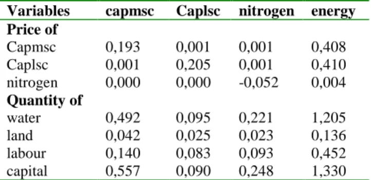
Table 1 provides short run price and input elasticities for 1994. Results show that own-price elasticities are positive for outputs and negative for variable inputs. In the short run, price elasticities are small. Input elasticities also are small, except for energy responses to water and capital intensities. This result is not unexpected. Mendes (1994a,b) has shown inelastic response of farmers in this area. Small and part-time farms are prominent in the EDM. Costa (forthcoming) shows that small farm milk price response is more inelastic in the presence of off-farm employment.

In the short run, demand for nitrogen increases weakly with respect to the prices of outputs, decreases with respect to its own price, and increases with respect to fixed inputs, particularly water and capital. Nitrogen and fixed inputs are complements.

Table 2 shows the long run elasticities for 1994 prices and virtual prices. Own-price elasticities are positive for outputs and negative for variable inputs, as expected. Usually, long run price elasticities

7 _{Constant Returns to Scale (CRS) in fixed inputs allows the derivation of a regional short run profit function from aggregation}

of the restricted profit model. Shadow prices of fixed inputs imply CRS in fixed inputs in the second stage. Regional virtual prices of fixed inputs are computed as weighted averages of representative farm shadow prices of fixed inputs.

are small. Nonetheless, they are more elastic than short run elasticities, as implied by the Le Chatelier Principle.

Demand for nitrogen increases weakly with respect to the prices of outputs (relatively more with respect to capmsc), decreases with respect to its own price and with respect to the prices of water, land, labor, and capital. In the long run, nitrogen is a complement to water, land, labor and capital, as it was in the short run. Responses to the prices of water and labor are more elastic than nitrogen responses to the other prices.

Demand for water increases with respect to the prices of outputs and decreases with respect to the prices of nitrogen and their own price. The own price elasticity for water is elastic, in the long run. The 1994 CAP was supporting in the EDM region agricultural commodities that used inputs more intensively, particularly water and nitrogen.

Table 1 - EDM short run agricultural elasticities

Variables capmsc Caplsc nitrogen energy Price of Capmsc 0,193 0,001 0,001 0,408 Caplsc 0,001 0,205 0,001 0,410 nitrogen 0,000 0,000 -0,052 0,004 Quantity of water 0,492 0,095 0,221 1,205 land 0,042 0,025 0,023 0,136 labour 0,140 0,083 0,093 0,452 capital 0,557 0,090 0,248 1,330

Table 2 - EDM long run agricultural elasticities

Variables capmsc caplsc nitrogen energy water land labor capital Price of capmsc 0,236 0,011 0,020 -0,549 0,630 0,518 0,267 0,776 caplsc 0,010 0,208 0,005 -0,106 0,115 0,292 0,148 0,120 nitrogen -0,001 0,000 -0,053 0,023 -0,010 -0,010 -0,006 -0,012 water -1,617 -0,276 -0,608 -3,691 -1,416 0,000 0,000 0,000 land -0,024 -0,014 -0,012 0,366 0,000 -0,270 0,000 0,000 labour -1,124 -0,641 -0,689 -2,652 0,000 0,000 -3,744 0,000 capital -0,257 -0,036 -0,093 -0,589 0,000 0,000 0,000 -0,195 CONCLUSIONS

A dual flexible quadratic restricted profit model was used to characterize EDM agriculture. The positive mathematical programming (PMP) approach was followed. In the context of the profit model, PMP has two stages. In the first stage, shadow prices of fixed inputs were obtained from a linear program that forces base year (1994) net output and fixed input allocations. In the second stage, the Maximum Entropy technique was used to recover twelve flexible quadratic restricted profit functions. The model reproduces base year net outputs and fixed inputs. A restricted regional function was derived from aggregation of the model. The corresponding long run profit function was also derived. In the second stage of PMP, twelve alternatives were considered for the support interval end points. These scenarios are based on expected elasticities. Price elasticities appeared more sensitive to specification of end points than input intensity elasticities because there is no price variability in the data whereas there is fixed input variability. Only two alternatives resulted in elasticities consistent

___________________________________________________________________________ with economic theory. These two alternatives generated similar elasticity results. Results are based on the average values from these two alternatives.

The profit model reveals an inelastic response to prices in the short run, and a more elastic response in the long run. The inelasticity of nitrogen response to its own price precludes taxing nitrogen to control its use. In contrast, pricing water is an effective strategy, not only to control water use but also nitrogen use. The Water Framework Directive (WFD) recommends both strategies.

REFERENCES

Costa, L. (2001). The Control of Agricultural Water Use in Northwest Portugal. Department of Economics. Tucson, Arizona, The University of Arizona.

Costa, L. (forthcoming). Desemprego familiar e produção de leite no Entre Douro e Minho. Livro de homenagem ao Professor Baganha. L. Castro. Porto, Universidade Católica Portuguesa.

Cox, T. L. and M. K. Wohlgenant (1986). “Price and Quality Effects in Cross-Sectional Demand Analysis.” Amer. J. Agr. Econ. 68, 4(1986): 908-919.

Golan, A., G. Judge, et al. (1996). Maximum Entropy Econometrics: Robust Estimation with Limited Data. New York, John Wiley & Sons.

Howitt, R. E. (1995a). “Positive Mathematical Programming.” Amer.J.Agr.Econ., 77, May, pp 329-342.

Howitt, R. E. (1995b). “A calibration method for agricultural economic production models.” Journal

of Agricultural Economics, 46 (2), pp 147-159.

Lau, L. J. (1976). “A Characterization of the Normalized Restricted Profit Function.” Journal of

Economic Theory, 12, pp 131-163.

Lopez, R. E. (1985). “Structural Implications of a Class of Flexible Functional Forms for Profit Functions.” International Economic Review, Vol. 26, No. 3, October), pp 593-601.

Mendes, A. M. S. C. (1994a). “Factores Influenciadores da Oferta de Trabalho Agrícola Familiar: Estimação duma Função de Oferta de Trabalho para as Zonas do Vale do Sousa e do Baixo Tâmega.”

Revista de Ciências Agrárias, Vol. XVII, Nº 3, pp 53-70.

Mendes, A. M. S. C. (1994b). “Factores Influenciadores da Procura de Terra Agrícola para Arrendamento: Estimação duma Função de Procura de Arrendamento para uma Zona do Alto Minho.”

Revista de Ciências Agrárias, Vol. XVII, Nº 4, pp 67-75.

Monke, E., F. Avillez, et al., Eds. (1998). Small Farm Agriculture in Southern Europe: CAP Reform and Structural Change. Vermont, Ashgate Publishing Company.

Neary, J. P. and K. Roberts (1980). “The theory of household behavior under input rationing.”

European Economic Review, 13, pp 25-42.

Oude Lansink, A. and G. Thijssen (1998). “Testing among functional forms: an extension of the Generalized Box-Cox formulation.” Applied Economics, 30, pp 1001-1010.

Paris, Q. and R. E. Howitt (1998). “An Analysis of Ill-Posed Production Problems Using Maximum Entropy.” Amer. J. Agr. Econ., 80, February, pp 124-138.

Quiroga, R. E. and B. E. Bravo-Ureta (1992). “Short- and long-run adjustments in dairy production: a profit function analysis.” Applied Economics, 24, pp 607-616.

Quiroga, R. E., J. Fernandez-Cornejo, et al. (1995). “The economic consequences of reduced fertilizer use: a virtual pricing approach.” Applied Economics, 27, pp 211-217.

Rothbarth, E. (1941). “The measurement of changes in real income under conditions of rationing.”

Review of Economic Studies, 8, pp 100-107.

Squires, D. (1987). “Long-Run Profit Functions for Multiproduct Firms.” Amer. J. Agr. Econ., 69, August, pp 558-569.