Materials and neuroscience: validating tools for large-scale, high-density neural recording

(1)

Joana Sofia Pereira Neto

Mestre em Engenharia Biomédica

Materials and neuroscience: validating

tools for large-scale, high-density neural

recording

Dissertação para obtenção do Grau de Doutor em Nanotecnologias e Nanociências

Orientador: Doutor Pedro Miguel Cândido Barquinha,

Professor auxiliar, Faculdade de Ciências e

Tecnologia da Universidade Nova de

Lisboa

Co-orientador: Doctor Adam Raymond Kampff, Senior Research Fellow, Sainsbury Wellcome Centre, London, United Kingdom

Júri:

Presidente: Doutor Pedro Miguel Viana Baptista Arguentes: Doutor Henrique Leonel Gomes

Doutor Alfonso Renart

Vogais: Doutor Rui Alberto Garção Barreira do Nascimento Igreja

Doutor João Carlos Azevedo Gaspar

(2)

(3)

Joana Sofia Pereira Neto

Mestre em Engenharia Biomédica

Materials and neuroscience: validating

tools for large-scale, high-density neural

recording

Dissertação para obtenção do Grau de Doutor em Nanotecnologias e Nanociências

Orientador: Doutor Pedro Miguel Cândido Barquinha,

Professor auxiliar, Faculdade de Ciências e

Tecnologia da Universidade Nova de

Lisboa

Co-orientador: Doctor Adam Raymond Kampff, Senior Research Fellow, Sainsbury Wellcome Centre, London, United Kingdom

Júri:

Presidente: Doutor Pedro Miguel Viana Baptista Arguentes: Doutor Henrique Leonel Gomes

Doutor Alfonso Renart

Vogais: Doutor Rui Alberto Garção Barreira do Nascimento Igreja

Doutor João Carlos Azevedo Gaspar

(4)

(5)

iii

Materials and neuroscience: validating tools for large-scale, high-density neural recording

A Faculdade de Ciências e Tecnologia e a Universidade Nova de Lisboa têm o direito, perpétuo e sem limites geográficos, de arquivar e publicar esta dissertação através de exemplares impressos reproduzidos em papel ou de forma digital, ou por qualquer outro meio conhecido ou que venha a ser inventado, e de a divulgar através de repositórios científicos e de admitir a sua cópia e distribuição com objectivos educacionais ou de investigação, não comerciais, desde que seja dado crédito ao autor e editor.

(6)

(7)

v

This work was developed in the context of the Nanotechnology and Nanoscience PhD program, in collaboration with the Champalimaud Research Programme, Champalimaud Center for the Unknown, Lisbon, Portugal. The project was carried out at Departamento de Ciência dos Materiais, CENIMAT/I3N and CEMOP/Uninova, Caparica, Portugal, Champalimaud Center for the Unknown, Lisbon, Portugal, and Sainsbury Wellcome Centre, University College London, London, United Kingdom.

This work was supported by funding from the European Union’s Seventh Framework Programme (FP7/2007-2013) under grant agreement nr. 600925, and by the the Bial Foundation (Grant 190/12). Joana Neto was supported by the fellowship SFRH/BD/76004/2011 from Fundação para a Ciência e Tecnologia, Portugal, and a Visiting Research Fellow stipend from Sainsbury Wellcome Centre, University College London, London, United Kingdom.

(8)

(9)

vii

‘Sempre chegamos ao sítio aonde nos esperam’ José Saramago, A Viagem do Elefante

(10)

(11)

ix

Acknowledgements

The work presented in the next pages was developed through six years in two countries and three institutes. During this journey I had the privilege of meeting and working with extraordinary people from different academic backgrounds, what made this journey an exciting and rich learning experience.

First, I was given the unique opportunity to collaborate with the neuroscience community on the other side of the river. To Prof. Dr. Elvira Fortunato and Prof. Dr. Rodrigo Martins, I want to thank for the support given to bridge two different fields, materials science and neuroscience. To Pedro Barquinha, I want to thank for accepting me as a student and taking up this project. For his kindness and guidance during this journey.

To all my colleagues and friends from CENIMAT, DCM, Champalimaud Center for the Unknown and Sainsbury Wellcome Centre, I want to thank for all their support during this research. I have to give thanks to Lídia Santos, Joana Vaz Pinto and Tiago Monteiro for the enthusiastic and honest collaborations.

I also want to express my gratitude to the students who have collaborated with me and provided contributions for this work. I am grateful to Msc. Pedro Baião, Msc. Pedro Lacerda, Msc. Kinga Kocsis, Msc. Ana Crespo, Msc. Nuno Coelho, Msc. Júlio Costa, Msc. João Rosa, and Msc. Jesse Geerts.

Throughout these years, a lot of days and nights, were spent in the Intelligent Systems Lab. I have to give thanks to Gonçalo Lopes, the guy with a brig brain and even more bigger heart. This work was only possible because he was always there to help me. Also to Joana Nogueira and Lorenza Calcaterra, who always stayed with me, helped me during long surgeries, and made sure I was still breathing. To João Frazão, the guy who is ‘always right’ and helped me to overcome uncountable challenges. To George Dimitriadis, who taught me a lot about programming and the ‘knows’ and ‘unknowns’ in neuroscience. To Ataback Dehban, Danbee Kim and André Marques-Smith for the companionship and fruitful discussions.

To Adam R. Kampff for being a believer. He believed, even when I had myself lost hope. Thank you, for showing me, since the first day, the importance of opening ‘black boxes’. Also, I want to thank him for the support and guidance in the experiments design, interpretation of results, and manuscripts writing.

Finally, I want to thank to my family for all the patience and love, and to Guilherme, for understanding and supporting my love for science.

(12)

(13)

xi

Abstract

Extracellular recording remains the only technique capable of measuring the activity of many neurons simultaneously with a sub-millisecond precision, in multiple brain areas, including deep structures. Nevertheless, many questions about the nature of the detected signal and the limitations/capabilities of this technique remain unanswered.

The general goal of this work is to apply the methodology and concepts of materials science to answer some of the major questions surrounding extracellular recording, and thus take full advantage of this seminal technique.

We start out by quantifying the effect of electrode impedance on the amplitude of measured extracellular spikes and background noise. Can we improve data quality by lowering electrode impedance? We demonstrate that if the proper recording system is used, then the impedance of a microelectrode, within the range typical of standard polytrodes (~ 0.1 to 2 MΩ), does not significantly affect a neural spike amplitude or the background noise, and therefore spike sorting. In addition to improving the performance of each electrode, increasing the number of electrodes in a single neural probe has also proven advantageous for simultaneously monitoring the activity of more neurons with better spatiotemporal resolution. How can we achieve large-scale, high-density extracellular recordings without compromising brain tissue? Here we report the design and in vivo validation of a complementary metal–oxide–semiconductor (CMOS)-based scanning probe with 1356 electrodes arranged along approximately 8 mm of a thin shaft (50 μm thick and 100 μm wide). Additionally, given the ever-shrinking dimensions of CMOS technology, there is a drive to fabricate sub-cellular electrodes (< 10 μm). Therefore, to evaluate electrode configurations for future probe designs, several recordings from many different brain regions were performed with an ultra-dense probe containing 255 electrodes, each with a geometric area of 5 x 5 μm and a pitch of 6 μm.

How can we validate neural probes with different electrode materials/configurations and different sorting algorithms? We describe a new procedure for precisely aligning two probes for in vivo

“paired-recordings” such that the spiking activity of a single neuron is monitored with both a dense extracellular silicon polytrode and a juxtacellular micro-pipette. We gathered a dataset of paired-recordings, which is available online. The “ground truth” data, for which one knows exactly when a neuron in the vicinity of an extracellular probe generates an action potential, has been used for several groups to validate and quantify the performance of new algorithms to

(14)

xii automatically detect/sort single-units.

(15)

xiii

Resumo

A gravação extracelular é a única técnica que permite a medição da atividade de vários neurónios simultaneamente, em várias áreas do cérebro (incluindo estruturas profundas), com uma precisão temporal de sub-milisegundos. Todavia, permanecem sem resolução várias questões concernentes à natureza do sinal detetado e às capacidades/limitações desta técnica.

O presente trabalho visa a apresentação de respostas a algumas das principais questões por solucionar relacionadas com a gravação extracelular de atividade neuronal, recorrendo para o efeito, à aplicação de metodologia e conceitos da ciência dos materiais.

Uma das questões à qual se procurou responder é relativa ao efeito da impedância do microelétrodo na amplitude dos potenciais de ação e do ruído de fundo. Podemos aumentar a qualidade do signal ao diminuir a impedância do elétrodo? Através do presente projeto demonstrámos que, utilizando-se um sistema de gravação apropriado, a impedância de um microelétrodo, dentro do intervalo típico dos elétrodos comerciais (~ 0.1 a 2 MΩ), não afeta significativamente a amplitude do potencial de ação ou o ruído de fundo e, consequentemente, a atribuição de cada potencial de ação ao respetivo neurónio.

Não se afigura, porém, apenas relevante melhorar o desempenho de cada elétrodo individualmente, sendo fundamental o aumento do número de elétrodos numa única sonda neural, por forma a permitir a monitorização simultânea da atividade de um número mais elevado de neurônios com melhor resolução espaciotemporal. Como podemos alcançar gravação extracelular de alta escala e densidade sem comprometer o tecido cerebral? Visando esse propósito descrevemos o design e validámos in vivo uma sonda de varredura baseada em tecnologia CMOS com 1344 elétrodos e 12 elétrodos de referência, dispostos ao longo de uma agulha fina (50 μm de espessura e 100 μm de largura) com aproximadamente 8 mm de cumprimento.

Considerando as dimensões cada vez menores alcançadas com a tecnologia CMOS, verifica-se uma tendência para fabricar elétrodos cada vez menores, com dimensões sub-celulares (<10 μm). Com efeito, para avaliar possíveis configurações dos elétrodos tendo em vista a produção de futuras sondas, realizámos gravações de diferentes áreas do cérebro com uma sonda ultradensa contendo 255 elétrodos, cada um dos quais com uma área geométrica de 5 x 5 μm e distância centro-a-centro de 6 μm.

(16)

xiv

diferentes algoritmos de classificação? Como resposta a esta questão descrevemos um novo procedimento para alinhar, com precisão, duas sondas para, posteriormente, gravar in vivo com ambas a atividade de um único neurónio, uma das quais uma agulha de silício com uma matriz densa de elétrodos e a outra uma micro-pipeta juxtacelular. Reunimos um conjunto de gravações nas quais ambas as sondas detetam o sinal do mesmo neurónio, as quais foram disponibilizadas

on-line. As referidas gravações nas quais se obtiveram sinais extracelulares em que se mediram os potenciais de ação gerados por um neurônio na proximidade, foram utilizadas por vários grupos para avaliar e quantificar o desempenho de novos algoritmos com vista à deteção/classificação de neurónios.

(17)

xv

List of Figures

Figure 1.1 Historical summary highlighting the ties between tools and discoveries in

neuroscience. ... 2

Figure 2.1 Graphical overview of the introduction where each panel highlights the main topics discussed throughout Chapter 2. ... 8

Figure 2.2 Neurons: the building blocks of brains. ... 12

Figure 2.3 Electric potential generated by current sources in a conductive volume. ... 13

Figure 2.4 Circuits to measure potential differences caused by flow of ions. ... 15

Figure 2.5 Diagram showing the modules of a typical recording system that contribute to the recorded voltages. ... 17

Figure 2.6 The electrical double layer at an electrode surface. ... 18

Figure 2.7 Electrochemical characterization of the electrode-solution interface. ... 20

Figure 2.8 Circuit diagram used by Ferree et al. for understanding the relationship between electrode impedance and amplifier input impedance. ... 23

Figure 2.9 Extracellular neural probes are fabricated with increasing number of electrodes to capture the activity of increasing number of neurons. ... 29

Figure 3.1 SEM images showing the surface morphology of electrodes from a commercial polytrode in their original state, and after the coatings. ... 37

Figure 3.2 Impact of impedance on data quality. ... 40

Figure 4.1 Circuits manufactured with CMOS technology. ... 45

Figure 4.2 NeuroSeeker CMOS-based probe. ... 48

Figure 4.3 Example of insertion coordinates adjustment for an animal larger than the dimensions presented by the brain atlas (B-IArat = 12.4 mm and B-IAAtlas= 9 mm). ... 49

(20)

xviii

Figure 4.4 Example of a recording performed with 1120 electrodes simultaneously within cortex,

hippocampus and thalamus from an anesthetized rat. ... 52

Figure 4.5 GPU visualization of the voltage traces from all (1060) electrodes in AP mode. ... 54

Figure 4.6 T-sne embedding of the kilosort algorithm (distances to templates) result for the recording 18_26_30.bin. ... 55

Figure 4.7 The 256-channel probe: dimensions, impedance and noise. ... 57

Figure 4.8 Acute recordings performed with a dense array of small electrodes in different brain regions. ... 58

Figure 5.1 In vivo paired-recording setup: design and method. ... 67

Figure 5.2 Paired extracellular and juxtacellular recordings from the same neuron. ... 70

Figure 5.3 Distance dependence of extracellular signal amplitude. ... 71

Figure 5.4 Extracellular detection of the juxtacellular neuron’s action potentials. ... 73

Figure 5.5 Spatiotemporal structure of extracellular signatures... 75

Figure 5.6 Dataset for validating spike detection and sorting algorithms for dense polytrodes. 77 Figure C.1 Example of a recording (18_26_30.bin) segment performed by a CMOS scanning neural probe with 1060 electrodes set to AP mode. ... 110

(21)

xix

List of Tables

Table A.1 Literature data used to investigate the relationship between the number of electrodes in neural probes and the number of neurons simultaneously recorded. ... 101 Table B.1. Summary of the dataset used to quantify the effect of electrode impedance on data quality. ... 103 Table C.1. Summary of the dataset used to validate CMOS-based probes. ... 104 Table C.2 Summary of the dataset gathered with the 256-channel probe. ... 105

(22)

(23)

xxi

Abbreviations

AC alternating current ADC analog-to-digital converter Ag-AgCl silver-silver chloride electrode AP action potential

B bregma

c cortex

CE counter electrode

cg cingulum

CIS CMOS image sensor

CMOS complementary metal-oxide-semiconductor DAC digital-to-analog converter

DC direct current

DMUX de-multiplexer

EDL electrical double layer

EIS electrochemical impedance spectroscopy FET field-effect transistor

fs sampling frequency

G1 to G12 group 1 to group 12

GND ground

GPU graphics processing unit

h hippocampus HD high definition IA interaural line IC integrated circuit IM intramuscular IP intraperitoneal

ISI interspike interval IVM in-vivo manipulator

JTA juxtacellular triggered average LFP local field potential

(24)

xxii

MOSFET metal-oxide-semiconductor field-effect transistor MUX multiplexer

NMOS n-channel metal-oxide-semiconductor P2P peak-to-peak amplitude

PBS phosphate buffer saline solution PCB printed circuit board

PEDOT-PSS poly(3,4-ethylenedioxythiophene) - polystyrene sulfonate PETH peri-event time histogram

PMOS p-channel metal-oxide-semiconductor

PS patchstar

RE reference electrode RMS root-mean-square

SC subcutaneous

SCE saturated calomel electrode SEM scanning electron microscopy SHE standard hydrogen electrode SNR signal-to-noise ratio

t thalamus

t-sne t-student stochastic neighbour embedding WE working electrode

(25)

xxiii

Symbols

Au gold

Cd capacitance of an ideal polarized electrode

Ce capacitance of the electrical double layer

Ci capacitance of the integrating capacitor

CSCE capacitance of an SCE electrode (reference electrode)

Csh shunt capacitance to ground from the electrode to the input of the amplifier

d1 thickness of the Helmholtz layer

E voltage source

f1 and f2 lower and upper limits of frequency bandwidth

i current measured

I current source

Ir iridium

IrOx iridium oxide

k Boltzmann’s constant

K+ _{potassium ion}

Na+ _{sodium ion}

Pt platinum

Re leakage resistance due to charge carriers crossing the electrical double layer

re position in space where potential Ve is measured

Rm resistance of the metallic portion

Rs resistance of the solution

Rsh shunt resistance to ground from the electrode to the input of the amplifier

Rz resistance of a large resistor

T temperature

Ti integration time

TiN titanium nitride

V potential measured

Ve potential created in the volume conductor with respect to a point at infinity

Ve’ potential at the input of the amplifier from the electrode

Vrec potential difference between Ve’ and Vref’

(26)

xxiv

Vref’ potential at the input of the amplifier from the reference

X, Y and Z axes

Z impedance

Z’ real part of the impedance Z’’ imaginary part of the impedance Za amplifier input impedance

Za_e’ effective amplifier input impedance for the electrode

Za_ref’ effective amplifier input impedance for the reference

Ze’ effective electrode impedance

Zref’ effective reference impedance

ρ extracellular conductivity

σ background noise

Φ electric potential

φ phase shift

ω angular frequency (rad s-1₎

(27)

1

Chapter 1. Motivation

Summary

In this dissertation we focus on extracellular recording, the oldest technique used to measure brain activity. Extracellular microelectrodes are used to measure the activity of neurons from outside the cell membrane at the sub-millisecond time scale. Recently, neural probes with thousands of microelectrodes have become available, allowing one to simultaneously observe the activity of hundreds, or even thousands, of neurons. Despite these incredible technological advances, many questions about the nature of the detected signal and the limitations of this technique remain unanswered. Hence, the motivation for this work arrives from the need to better understand the neural probes used for large-scale, high-density extracellular recordings, and thus explore their full potential. Finally, this chapter ends with overall research goals and an outline of the thesis.

(28)

2

1.1 Scientific context: sensing neuronal activity from the extracellular space

We currently lack a theory describing how the brain works (Krioukov, 2014). Efforts have thus focused on creating techniques and tools capable of advancing our understanding of the physiological properties of the nervous system. Today, extracellular recording remains the only technique capable of measuring the activity of many neurons simultaneously with sub-millisecond precision in multiple brain areas, including deep structures (e.g., thalamus).

In the 1920s, Edgar Adrian measured extracellularly the signals transmitted to the brain from single sensory nerve fibres, and described how these signals were related to the stimulus which produced them (i.e., pressure on the muscle). These signals were found to use a common vocabulary. They consisted of a series of brief and uniform changes in electric potential (so-called action potentials or spikes) (Adrian, 1928).

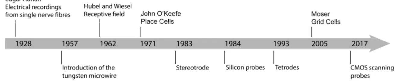
Figure 1.1 Historical summary highlighting the ties between tools and discoveries in neuroscience. The development of extracellular microelectrodes enabled researchers to monitor the activity pattern of individual neurons in relation with external stimuli and behavior. The diagram shows the introduction of new tools (Hubel, 1957; McNaughton, O’Keefe, & Barnes, 1983; Najafi, Wise, & Mochizuki, 1985; O’Keefe & Recce, 1993; Takahashi & Matsuo, 1984; Wilson & McNaughton, 1993) together with the key findings resulting in Nobel Prize awards in neuroscience (Adrian, 1928; Hubel & Wiesel, 1962; O’Keefe & Dostrovsky, 1971; Hafting, Fyhn, Molden, Moser, & Moser, 2005). Adapted from Yuste, 2015.

Since Adrian, quantifying brain activity (spikes from individual cells), and its relationship to sensory and behavioural variables, has become the cornerstone for understanding brain function (Hafting et al., 2005; Hubel & Wiesel, 1962; O’Keefe & Dostrovsky, 1971). A thin insulated metal microwire with an exposed tip have become the tool of choice to measure action potentials of single neurons in the brains of behaving animals, since pioneering studies of the 1950s (Figure 1.1). The focus on the properties of individual neurons was a natural consequence of the use of a single microelectrode (Hubel, 1957). Over the years, technological progress has contributed to a move from microwires (McNaughton et al., 1983; O’Keefe & Recce, 1993) to microfabricated silicon probes with dozens of microelectrodes, also called polytrodes (Najafi et al., 1985; Takahashi & Matsuo, 1984).

(29)

3

Today, CMOS-based probes with thousands of microelectrodes packed in a high-density array are being developed using modern methods for integrated circuit design and fabrication. Why do researchers need thousands of microelectrodes? The number of simultaneously identified neurons in a single experiment largely depends on the number of individual microelectrodes on the neural probe (Stevenson & Kording, 2011) and many neuroscientists hope that simultaneously monitoring the activity of more individual neurons will help us to understand how the constituent parts of the nervous system lead to the emergent properties of the whole behaving organism (Buzsáki, 2004). A helpful metaphor is our visual comprehension of an image presented to us on a computer screen. Imagine that someone is trying to comprehend the image by looking at individual random pixels. This task is almost impossible to accomplish with view of only a small number of pixels, and to decipher the image, it is important to simultaneously view as many pixels as possible (Yuste, 2015).

However, one must remember that extracellular recordings are an imperfect representation of the underlying neuronal activity (Harris, Quiroga, Freeman, & Smith, 2016; Moore-Kochlacs, 2016; Shoham, O’Connor, & Segev, 2006). Each microelectrode captures a mixture of activity from multiple neurons together with noise. Noise sources, both of biological (e.g., electric activity from neurons further away the recording microelectrode) and non-biological (e.g., thermal noise) origin, contribute for the background noise.

“What contributes to the amplitude of action potentials as well as the background noise? Can we improve data quality by physical design choices (e.g., the individual microelectrode impedance and size)? How will these be reflected in the subsequent sorting analysis? What arrangement of electrodes is optimal for isolating individual neurons from background noise? How can we validate probes with different electrode configurations and different sorting algorithms? How can we achieve the full potential of large-scale, high-density extracellular recordings?”

This work aims to settle such questions as they relate to extracellular recording, and to help researchers take full advantage of this seminal technique.

(30)

4

1.2 Research goals

In order to understand and achieve the full potential of neural probes (with dozens, or even thousands, of microelectrodes) used for large-scale, high-density extracellular recordings, the research was split into four main tasks:

1) Identify the factors that govern the efficiency of signal transfer from the neuronal activity into digital recorded voltages;

2) Quantify the effect of electrode impedance on the amplitude of measured extracellular spikes and background noise;

3) Validate a large-scale, ultra-high density CMOS-based probe developed in collaboration with the NeuroSeeker consortium. These CMOS probes represent a major innovation, but also a major challenge for current analysis methods. Additionally, due to the ever-shrinking dimensions of CMOS technology, validate electrode configurations for future probe designs;

4) Develop a method for efficiently gathering “ground truth” data to quantify the performance of different electrode configurations and spike sorting methods.

1.3 Thesis outline

The structure of the work presented in this dissertation follows the order of the tasks described above, and in each of the chapters we set out to accomplish one of the mentioned tasks.

In Chapter 2 we provide some fundamental background regarding the operating principles of extracellular recording, highlighting the factors that can affect the extracellular recording voltages, and subsequent analysis.

In Chapter 3 we discuss how a commercial electrode impedance affects data quality in spikes recording. We compare, side-by-side, the same extracellular signals measured by coated (low impedance) microelectrodes and non-coated (high impedance) microelectrodes.

In Chapter 4 we report the design and in vivo validation of a CMOS-based scanning probe with 1356 electrodes arranged along approximately 8 mm of a thin shaft. We also present new methods for analysing large-scale extracellular recordings. Additionally, to evaluate electrode configurations for future probe designs (i.e., electrode size, density and geometry), several recordings from many different brain regions were performed with an ultra-dense probe containing 255 electrodes, each with a geometric area of 5 x 5 μm and a pitch of 6 μm.

(31)

5

In Chapter 5 we describe a procedure for precisely aligning two probes for in vivo “paired-recordings” such that the spiking activity of a single neuron is monitored with both a dense extracellular silicon polytrode and a juxtacellular micro-pipette.

Finally, in Chapter 6 we discuss the implications of our experimental findings and the future of extracellular recordings.

(32)

(33)

7

Chapter 2. General Introduction

Summary

Herein, our goal is to make intelligible the factors that govern the efficiency of signal transfer, from the brain to a digital record using extracellular recordings. Therefore, we provide some fundamental background regarding the operating principles of extracellular recordings and the electrode-brain interface. We also describe the challenges for analysis of an extracellular recording. Finally, this chapter ends with a brief historical perspective on extracellular microelectrodes, and the new technologies that will probably shape the field of recording tools for brain research.

(34)

8

2.1 In Brief

Figure 2.1 frames the introduction and will serve as a guide throughout the discussion of different topics in this chapter.

Figure 2.1 Graphical overview of the introduction where each panel highlights the main topics discussed throughout Chapter 2. (a) 2.2 Brain, neurons and extracellular space; (b) 2.3 Neuronal activity, extracellular currents and potentials; (c) 2.4 Extracellular recording systems; (d) 2.5 Microelectrode-extracellular space interface and impedance measurement; (e) 2.6 Effects of the electrode impedance on data quality; (f) 2.7 Effects of electrode size on data quality; (g) 2.8 Effects of electrode density on spike sorting algorithms; (h) 2.9 Large-scale recording of neuronal activity.

(35)

9

Neurons are the building blocks of the brain, and they are connected together into networks that process information within milliseconds. Figure 2.1a shows a section of the rat brain (our model organism) where each densely packed dot is a neuron cell body. Brain tissue comprises neural cell bodies (somas), connecting fibres (axons and dendrites), glial cells, and blood vessels. When a neuron is active, transient changes in its membrane cause currents (ionic and capacitive) to flow into and out of the cell (Figure 2.1b). The strongest and fastest currents across the neural membrane are caused by Na+_{ions rushing into the cell at the start of an action potential, followed}

by an outward flow of K+_{, which co-occurs with a small capacitive current across the entire cell}

membrane as the membrane is charged by the influx of Na+_{ions at the initial segment of the axon}

(marked in orange). Each of these transmembrane currents superimpose in the extracellular medium (which acts as a volume conductor), defining an electric potential field. To detect the presence of an active neuron, we measure the electric potential (Ve) in the extracellular space

near the neuron, relative to some distant reference. The activity of a neuron generates a stereotypical temporal deflection of the electric potential, known as an extracellular action potential, or a spike. The largest electric potential deflection occurs near the initial segment of the axon.

Therefore, in extracellular recordings, the recorded voltage (Vrec) reflects the potential difference

between a microelectrode that is usually inside the brain, close to neurons, and the reference electrode. Our goal is to position our recording electrode as close as possible to the soma. Note that the recorded signal imperfectly represents what is happening around the cell because each electrode captures the spiking activity of several neurons in its vicinity together with noise. Moreover, the recorded electric potential will also depend on the recording system. Currently, the entire recording system is composed of the microelectrode(s), reference electrode and the hardware connected to them, including amplifiers, filters and analog-to-digital converters (ADCs) (Figure 2.1c). The amplification of the potential difference between the microelectrode and the reference electrode (on the order of microvolts) is a crucial step, and is accomplished with differential amplifiers that amplify the differences, rejecting the noise that is often introduced as common-mode potential in the circuit.

The mechanism that underlies the transduction of the neuronal activity into recorded voltages begins with the electrode-extracellular interface. In Figure 2.1d the effective electrode impedance (Ze’) is the sum of the resistance of the solution (Rs), the resistance of the electrode metal (Rm),

and the resistance (Re) and capacitance (Ce) of the double-layer that forms on the metal

electrode-extracellular interface (i.e., the charge on the metal is equal and opposite to the total charge on the extracellular side of the interface).

(36)

10

The quality of the data depends on the amplitude of the extracellular action potentials relative to the background noise. What then contributes to the amplitude of the observed action potentials, as well as the background noise? One common confusion is how the electrode impedance affects the recorded signal, and therefore spike’s amplitude. To better understand the voltage drops and current pathways that occur in a recording system, a simplified circuit is shown in Figure 2.1e. The effective electrode impedance (Ze’) and effective amplifier input impedance (Za_e’) form a

voltage divider. The effective amplifier input impedance is the total impedance to ground, as seen from the electrode, and it includes a path through the amplifier and shunting routes to ground. Therefore, as long as the input impedance amplifier is larger than the impedance of the electrode-extracellular interface, the voltage drop in the electrode-extracellular interface is neglected and the potential difference at the amplifier inputs should reflect the actual difference in electric potential, Ve- Vref.

A separate question from whether the impedance of an electrode influences the recorded voltage, is the question of whether the size of the recording site has an impact on the recorded spikes. Larger electrodes can reduce the signal amplitude due to the averaging with nearby regions with smaller signals. High density arrays of small electrodes (5-20 μm) can reduce spatial averaging of action potentials and increase the probability of finding “the sweet spot” near a neuron’s soma (Figure 2.1f). When using small electrodes, the only limiting factor is electrode noise, which scales as a factor of size. How small can you make recording electrodes? Decreasing electrode size lowers electrode capacitance and increases its resistance, both increasing impedance, which increases thermal noise. On top of the thermal noise, biological noise (i.e., the activity of many distant neurons) also adds to the noise background magnitude.

The data quality is important for the subsequent steps of detection and isolation where spike sorting algorithms extract and identify the activity of individual neurons from the extracellular voltage traces. In our recording devices, besides the impedance and size of electrodes, another physical design choice, can play an important role in the subsequent analysis - the density and arrangement of the electrodes (Figure 2.1g). What arrangement of electrodes is optimal for isolating individual neurons from background activity?

To understand how the brain works, possibly we will need to simultaneously record and analyse a large number of neurons from different brain areas. Extracellular probes have been fabricated with an increasing number of electrodes in order to capture the activity of an increasing number of neurons. In 2017, the European project NeuroSeeker resulted in the development of probes with 1356 electrodes on a single 8 mm shank, which allowed us to record in vivo the activity of hundreds of neurons across several structures in the brain (Figure 2.1h).

(37)

11

2.2 Brain, neurons and extracellular space

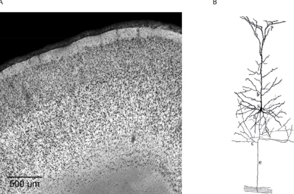
In the eighteenth century, the individual components of which the whole brain is built were finally revealed by Santiago Ramón y Cajal under the microscope, after adapting the Golgi staining protocol (Kandel, Schwartz, & Jessel, 2000). In Texture of the Nervous System of Man and the Vertebrates, Ramón y Cajal presented detailed drawings of brain cells scattered across different brain regions (Ramon y Cajal, 1899). In Figure 2.2b we can see several connecting fibres (dendrites and axon) growing out from the cell body. Each neuron may establish direct contact with thousands of other neurons through specialized communication sites called synapses. In general, each neuron receives input from many other neurons through dendritic synapses, while sending its own output through the axon, which can establish synapses with a large population of other brain cells (Eccles, 1973). In Figure 2.2a only the neuron cell bodies are stained black, unlike the Golgi staining used by Ramón y Cajal (Figure 2.2b). If all the dendrites and axons from every neuron were stained in a slice of brain tissue, the result would be a solid black picture. A rat brain has about 200 million (and a human brain has about 86 billion) neurons tightly packed together (Azevedo et al., 2009; Herculano-Houzel, 2009). The density in the rat cortex, according to the literature, is between 40,000 to 100,000 neurons per mm3 _{(DeFelipe, Alonso-Nanclares, &}

Arellano, 2003; Markram et al., 2015; Meyer et al., 2010). In addition to neuronal cell bodies, axonal fibres, and dendritic structures, the brain also contains glial cells and blood vessels. Thus very little of the extracellular space is actually “space”. Indeed, extracellular fluid is thought to comprise only 12–25 % of the brain’s volume (Li et al., 2015; Nelson, Bosch, Venance, & Pouget, 2013; Tønnesen, Inavalli, & Nägerl, 2018).

Cajal once described the brain as an ‘impenetrable jungle where many investigators have lost themselves’ (Ramon y Cajal, 1923). However, it is through these large and distributed neural networks that the brain runs, builds and stores detailed models of the world, and continuously adapts them to new environments (Nicolelis, 2011).

(38)

12

Figure 2.2 Neurons: the building blocks of brains. (a) Nissl-stained section of the rat cortex. All neuron cell bodies (somas) are stained; (b) Drawing by Ramon y Cajal from pyramidal cell of the rabbit cerebral cortex. In the pyramidal cell, ‘a’: basal dendrites, ‘b’: dendritic trunk and its branches, ‘c’: axon collaterals, ‘e’: long axon, ‘P’: apical dendrites, and ‘s’: soma. Adapted from Ramon y Cajal, 1899. More recent studies on cortex cell morphology and function are available (Jiang et al., 2015; Markram et al., 2015).

2.3 Neuronal activity, extracellular currents and potentials

Neuronal activity gives rise to transient changes in the flow of current into and out of the cell.

Briefly, when an input signal (a receptor potential or synaptic potential) depolarizes the cell membrane, this change in membrane electric potential opens Na+_{ion channels, allowing Na}+_to

flow from outside the cell, where the Na+_{concentration is high, to the inside of the cell, where}

Na+ _{concentration is low (Kandel, Schwartz, & Jessel, 2000). In neurons, voltage-sensitive Na}+

channels are usually concentrated at the initial segment of the axon (marked in orange in Figure 2.1b). Therefore, it is more likely that the action potential arises at the initial segment of the axon, rather than in other regions of the cell. The sudden influx of Na+_{ions through these}

voltage-sensitive channels in the cell membrane upsets the balance of processes that maintain the neuron at its resting equilibrium, and leads to a series of further changes which constitute the action potential (Hodgkin & Huxley, 1939).

All of the transmembrane currents within a volume of brain tissue superimpose in the extracellular medium (re), and generate a potential, Ve (a scalar measured in Volts), with respect

(39)

13

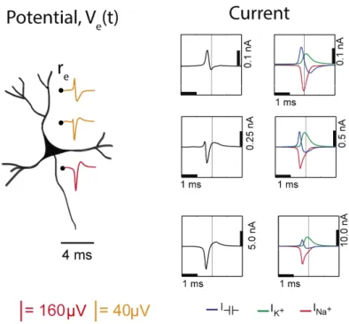
to a point at infinity (Figure 2.3). By infinity we mean a location that is far from all of the sources of electric potential (Einevoll, Kayser, Logothetis, & Panzeri, 2013). The electric field and therefore the potential Ve induced in a volume conductor by the transmembrane currents

depends on the magnitude, sign and location of the current sources, and on the conductivity of the extracellular medium (Buzsáki, Anastassiou, & Koch, 2012; Nunez & Srinivasan, 2009). Figure 2.3 depicts the time-varying extracellular potential at given locations (re) that resulted from

the superposition of the ionic and capacitive transmembrane currents formed when a neuron was active. The difference in potential waveforms at different locations in the extracellular medium is mainly given by the shape of the net current (Figure 2.3, first column) across the membrane. Furthermore, the peaks in the potential waveforms correspond to the current (Figure 2.3, second column) that is dominant at that time-point: the first positive peak of the waveform is attributed to the positive capacitive current resulting from the strong Na+_{current entering the}

axon initial segment; the main negative peak is attributed to the influx of Na+

; and finally, the second positive peak results from repolarizing K+_{current flowing out of the cell (Gold, Henze,}

Koch, & Buzsáki, 2006).

Figure 2.3 Electric potential generated by current sources in a conductive volume. The extracellular potentials and currents are adapted from Gold et al., 2006. Extracellular potential waveforms at selected spatial positions, re (marked with black dots) are simulated for a CA1 pyramidal neuron. Currents: simulated net membrane current

(first column) across the soma and proximal dendrites that best estimates the extracellular potential waveform and membrane current components in terms of Na+_{, K}+_{and capacitive currents (second column). In the soma,}

the positive capacitive current coincides with the larger Na+_{current. At locations along the apical trunk, the initial}

capacitive peak becomes visible. In dendritic compartments the membrane depolarization is initially driven by Na+_{current from the soma, until local Na}+_{currents are activated and the action potential regenerates. In the brief}

time before the local Na+_{currents activate, the positive capacitive current is the dominant membrane current and}

(40)

14

In more detail, the extracellular potential Ve at position re can be computed with the following

equation, described in several works (Einevoll et al., 2013; Nunez & Srinivasan, 2009; Pettersen, Lindén, Dale, & Einevoll, 2010), as:

𝑽_𝒆(𝒓_𝒆, 𝒕) = 𝟏 𝟒𝝅𝝆 𝑰_𝒏(𝒕) |𝒓_𝒆− 𝒓_𝒏| 𝑵 𝒏 𝟏 Equation 2.1

Conceptually, the point-source equation (Equation 2.1) is key for computing the extracellular potential in response to any transmembrane current (Buzsáki et al., 2012). In(t) represents the nth

point current source and re – rn represents the distance between the point source and the position

of measurement, with n = 1...N, where N is the number of individual point sources and ρ is the extracellular conductivity. If the extracellular medium is considered homogeneous and isotropic that means a constant conductivity value (Einevoll et al., 2013).

Therefore, to detect the presence of an active neuron nearby in the extracellular space, the electric potential relative to some distant reference point must be measured. The model presented in Figure 2.3 illustrate how the electric potential varies nearby an active neuron. The extracellular potential waveforms usually last on the order of 1-2 ms, and are in the range of tens to hundreds of microvolts in amplitude, with the largest potential deflections being detected close to the soma of a neuron. These stereotypical temporal deflection of the electric potential in the extracellular space are called action potentials or spikes.

2.4 Extracellular recording systems

In Figure 2.1c, an extracellular recording in rat cortex under anesthesia is represented as Vrec.

This voltage trace contains 40–500 μV action potentials (1 ms wide) from a population of neurons nearby, as well as slower fluctuations that range from tens to thousands of microvolts. The low-frequency band of the recorded signal (< 300 Hz) contains local field potentials (LFPs) that reflect synchronized synaptic currents. The idea that synaptic currents contribute to the LFP stems from the recognition that extracellular currents from many individual neurons must overlap in time to induce a measurable signal, and such overlap is most easily achieved for relatively slow events, such as synaptic currents (Buzsáki et al., 2012; Einevoll et al., 2013). Since, our focus is on the fast voltage deflections known as spikes, the lower frequency signal is separated from the spike

(41)

15

signal by high-pass filtering around 250 Hz (Buzsáki et al., 2012; Schomburg, Anastassiou, Buzsáki, & Koch, 2012).

As shown in Figure 2.1b and c, the voltage measured (Vrec) should reflect the potential difference

between a microelectrode close to a neuron and a reference electrode at a much larger distance from all the current sources. The potentials Ve and Vref are the potentials just below the electrodes’

interface and are also the voltages impressed at the microelectrode and reference, respectively. As mentioned above in 2.3 Neuronal activity, extracellular currents and potentials, the Ve is

created in the volume conductor by the transmembrane currents. In an ideal recording system the Vrec will be equal to Ve – Vref, and it will be the potential difference that would exist if the tip

had no net current flowing into it (Robinson, 1968). However, the recorded voltage Vrec relies on

a recording system. Currently, for recording extracellular activity, researchers use a system composed of electrodes (i.e., microelectrode(s) and reference), amplifiers, filters, and digitizers, and finally software to visualize, save and analyze data. Here we will focus on the acquisition of extracellular action potentials measurements.

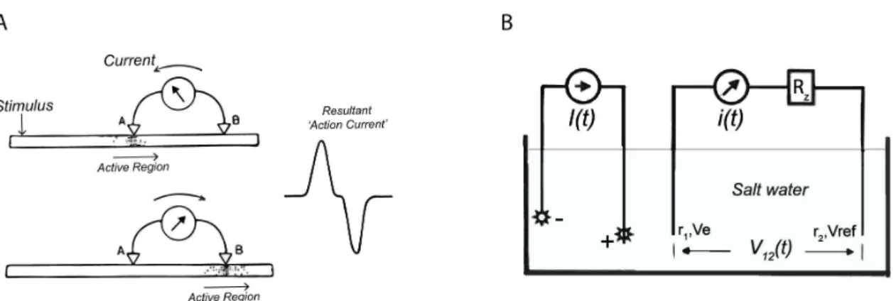
Figure 2.4 Circuits to measure potential differences caused by flow of ions. (a) A simple circuit to detect potential changes in nerves using a galvanometer. Adapted from Adrian, 1928; (b) A current source I(t) generates a potential field in a salt water tank. The circuit to record reliably the potential difference between Ve at location r1

in the tank with respect to a ‘reference’ electrode Vref at location r2, needs to meet two conditions: first, the

resistance (Rz) is much larger than the impedance of the salt water plus electrode-salt water interface plus the

galvanometer resistance, so that the small measured current i(t) is simply related with V12(t), and second, the

current i(t) must be large enough to meet the sensitivity requirement of the current instrument, but small enough to avoid distorting the potential field (Nunez & Srinivasan, 2009).

The first recording of action potentials, also called ‘action currents’, was performed in nerves using galvanometers (see Figure 2.4a). This very simple measurement system can be created by connecting an electrode in series with a galvanometer to a reference electrode. This defines a simple circuit, where the potential difference between the electrode and the reference drives a current in the galvanometer. However, the current flowing in this circuit can distort the potentials that are being measured. The use of relatively high current movements can load the voltage under

(42)

16

test, giving incorrect readings. One simple solution to this problem is to connect a large resistor in series with the galvanometer as shown in Figure 2.4b. This defines a circuit, where the potential difference between the electrode and the reference is given by Ohms law (Ve – Vref = V12 = i(t) Rz).

Unfortunately, this recording system configuration does not offer sufficient sensitivity (potential differences are less than 1 mV) for recording the potential variation from a single neuron. Edgar Adrian in The Basis of Sensation wrote: ‘A great deal of the difficulty in physiological research is due to the microscopic size of the living cell – the unit out of which the organism is built. … all the changes which we wish to investigate are very small too, and the experiments, which would be simple enough theoretically, are continually checked by the technical difficulties of work on a minute scale.’ He was one of the first to study the activity of the nervous system at a cellular level in the 1920s. How did he manage to accurately measure the potential changes resulting from the activity of a single neuron? Using a valve amplifier to magnify electric potential changes, he could record spikes in single nerve fibres (axons) (Adrian, 1928). Valve amplifiers were developed during the first World War for detecting wireless signals and were applied to physiological research as soon as the war was over (Nicolelis, 2011). It is important to note that the measurement of a ‘clean’ signal was possible with this recording system because the nerve was inside a metal box that shielded from electromagnetic disturbances (i.e., Faraday cage). Nowadays, to measure the faint signal arising from brain activity, recording systems are designed to amplify the potential difference between electrodes and to reject the common-mode potential (i.e., noise identical in the recording and reference electrodes typically caused by capacitive coupling of the body and electrode lead with power line fields (Nunez & Srinivasan, 2009)). Usually this is accomplished with differential amplifiers characterized by high input impedance and low noise (Ferree, Luu, Russell, & Tucker, 2001). In Figure 2.5, a simple recording system diagram shows all the modules of a typical recording system that contribute to the recorded voltages, including the differential amplifier.

(43)

17

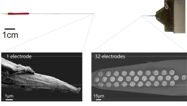
Figure 2.5 Diagram showing the modules of a typical recording system that contribute to the recorded voltages. Adapted from Intro to Intan Amplifier Chips | Intan Technologies, 2017. The signals from the electrodes are amplified and digitized with a sampling frequency in the range of 20–30 kHz. First, high-pass filters must be used to remove the large DC offsets present at the electrode-extracellular interface, along with any undesired low-frequency signals (e.g., movement artifacts). Second, high gain differential amplifiers are used to boost the signals to the larger voltage levels required by the ADC and to reject common-mode noise. Additionally, low-pass filters must be configured to less than half of the ADC frequency sampling rate to prevent aliasing, and may also be used to block undesired high-frequency signals and artefacts (Intro to Intan Amplifier Chips | Intan Technologies, 2017). An example of a headstage from Intan wich allows simultaneously recording from 32 microelectrodes. Adapted from Open Ephys, 2017.

2.5 Microelectrode-extracellular space interface and impedance measurement

The mechanism that underlies the transduction of neuronal activity into recorded voltages relies on the electrode-extracellular space interface.

Extracellular microelectrodes are usually made from metallic conductors. A thin insulated metal wire with an exposed tip is the most basic, and still widely used, device for in vivo extracellular recording from brains. Metals such as platinum, gold, tungsten, iridium, titanium nitride, stainless steel, iridium, iridium oxide, and alloys, nickel-chrome, platinum-iridium and platinum-tungsten have all been used in neural electrodes.

The measurement of electric potentials caused by the flow of ions in the extracellular space, where the conductivity is roughly six orders of magnitude lower than that in metals, is possible due to the transfer of ionic current, and the resulting potential, to the movement of electrons in

(44)

18

the metal electrode and lead connected to the external recording circuit. This transition from ion flow to electron flow is made through the double layer interface.

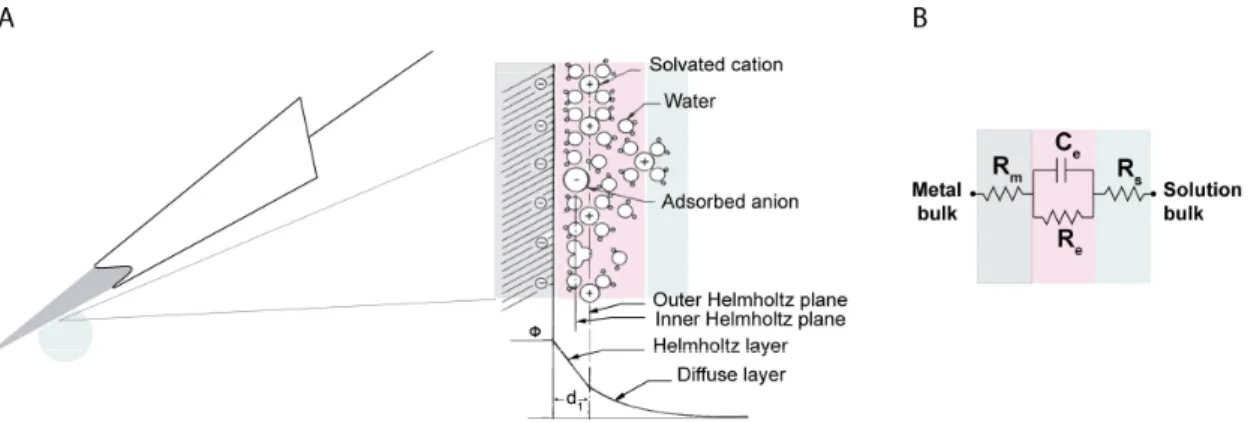
What is the double layer interface? When a metal is placed in a saline solution two phenomena occur: water dipoles close to the metal surface become oriented, and assuming the metal surface is negatively charged, the solution close to the metal surface become depleted of negative ions (anions), leaving behind a cloud of positive ions (cations). This cloud of cations screens the electric field caused by the excess of charge on the metal. Electroneutrality across the interface requires that the charge on the metal is always equal and opposite to the total charge on the solution side of the interface (Musa et al., 2012). The resulting charge distribution - two narrow regions of equal and opposite charge - is known as the electrical double layer (EDL).Figure 2.6a shows a model for the distribution of electric potential across a metal-solution interface, where the double layer region (represented in pink in the schematics) yields a capacitance, Ce which

typically has a value around 20 μF cm-2 _{(Musa, 2011).}

Figure 2.6 The electrical double layer at an electrode surface. Adapted from Wise, Angell, & Starr, 1970. (a) Electric potential (ϕ) profile across the double-layer region in the absence of specific adsorption of ions. The thickness of the Helmholtz layer, d1 is of the order of an ionic radius (2 to 4 Å). The potential difference between

the metal and the solution appears as DC offset in the measured signal and usually is removed by hardware high-pass filtering at 0.1 Hz. Thus, this potential difference known as the half-cell potential is established between the metal and the bulk of the solution; (b) Equivalent circuit model of the interface of a metal microelectrode recording in the brain. Adapted from Robinson, 1968.

The signal transduction takes place across the electrode-extracellular space when the charge distribution changes on the extracellular fluid side. In the previous section it was shown that ionic flow during the action potential gives rise to measurable time-varying electric potentials. The electric potential variation in the extracellular space is accompanied by a redistribution of the ion concentration close to the metal electrode and hence induce changes in the electrode’s charges. In Figure 2.6b we introduce a simple model of the solution interface. The electrode-solution interface can be represented by a parallel ReCe combination in series with the resistances,

(45)

19

with leakage resistance due to charge carriers crossing the electrical double layer. Ce is the

capacitance of the electrical double layer at the interface of the exposed metal and the solution. This model is strictly limited to small potentials being relevant for the case of neural recording where extracellular signals are in the order of a few hundred microvolts.

The transition from ion flow in the solution to electron flow in the electrode could be of capacitive nature, involving the charging and discharging of the electrode-solution double layer (purely electrostatic), or faradaic, in which surface-confined species are oxidized and reduced (Bard & Faulkner, 2001; Merrill, Bikson, & Jefferys, 2005).

Electrodes at which faradaic processes occur are called charge transfer electrodes or ‘non- polarized’. The well-known silver-silver chloride (Ag-AgCl) electrode approaches the ideal non-polarizable type. Moreover, non-non-polarizable electrodes have a small Re allowing charge-transfer

across the electrode-solution interface. If Re is small, it bypasses the capacitor Ce thus providing

a DC path for the measurement of steady potential levels. On the other hand, noble metals (e.g., stainless steel, gold and platinum) electrodes are so-called ‘polarizable’ electrodes and thus no charge transfer can occur across the metal-solution interface. Instead, electrode polarization is required to motivate current flow in the external recording circuit. The value of Re of polarized

electrodes is large, in the order of several megohms, and the effective equivalent circuit is dominated by the capacitor, Ce. Therefore, processes in polarizable electrodes are purely

electrostatic in nature and caused by the charging and discharging of the double layer capacitance. Although charge does not cross the interface, external currents can flow (at least transiently) when the potential or solution composition changes (Cooper, 1971).

If one is interested in evaluating the individual circuit elements of the electrode-solution interface, it is possible to perform an electrochemical characterization. One can fully describe the processes governing the electrode’s behaviour by applying an electrical perturbation to the system and measuring the response. The response of an electrode-solution interface can be modelled in terms of an equivalent circuit where the individual circuit elements describe the various phenomena occurring at the interface (Musa et al., 2012).

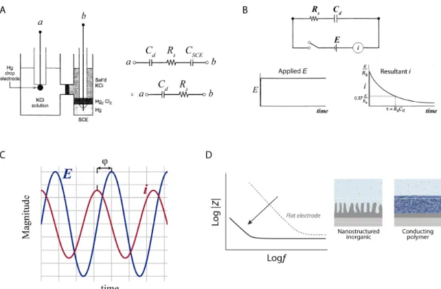
For example, consider a typical electrochemical experiment, as shown in Figure 2.7a, where an electrode under evaluation (working electrode) and a reference electrode are immersed in a solution, and the potential difference between them is varied by means of an external power supply.

(46)

20

Figure 2.7 Electrochemical characterization of the electrode-solution interface. (a) Two-electrode cell with an ideal polarized mercury drop electrode and a SCE reference electrode. Representation of the cell in terms of linear circuit elements. Adapted from Bard & Faulkner, 2001; (b) Current transient resulting from a potential step applied to the working electrode with respect to the reference. The Rs and Cd value can be computed from

i-E curves. Adapted from Bard & Faulkner, 2001; (c) Graphical representation of the time dependent sinusoidal current response to a small ac voltage; (d) Increasing the electrode surface area or coating the electrode with conducting polymers enables an increase of Ce value, and consequently a drop in impedance. The comparison

of impedance is shown for a flat electrode (gray, dotted) and for an electrode with an enhancing coating (black line; for example, conductive polymers). Adapted from Rivnay, Wang, Fenno, Deisseroth, & Malliaras, 2017. This system can be approximated by an electrical circuit with a resistor, Rs representing the

solution resistance and a capacitor, Cd representing the double layer interface of an ideal

polarized electrode. Usually, reference electrodes are made up of phases having constant composition (e.g., standard hydrogen electrode (SHE), saturated calomel electrode (SCE) and silver-silver chloride electrode (Ag-AgCl))(Bard & Faulkner, 2001).A reference electrode, such as SCE, approaches an ideal non-polarized where the passage of current does not affect its potential. Therefore, the contributions from the reference electrode are usually negligible. Herein, the variation in potential presented in Figure 2.7b, will produce a current to flow in the external circuit that depends on the circuit impedance and it reflects the response of the electrode, represented by the circuit elements Rs and Cd in series. The impedance is a measure

of the ability of a circuit to resist the flow of charge across the electrode-solution interface phases (i.e., electronic conductor and an ionic conductor).

Usually, impedance is measured by applying a time-varying sinusoidal voltage signal, E(ωt) = E0

(47)

21

ω (rad s-1_{) the angular frequency, and the current response is monitored, i(ωt) = i}

0 sin(ωt+φ) with

i0 being the current amplitude and φ the phase shift (see Figure 2.7c). The impedance can be

computed as E(ωt)/ i(ωt) and represented as a vector defined in terms of magnitude |Z| and phase shift φ. The measurement is made over a broad frequency range, typically from 1 Hz to 10 kHz, and the magnitude of the excitation is sufficiently small that a linear current-voltage response is obtained at each frequency (Cogan, 2008). In complex analysis, a projection of the vector on the x-axis is called the real part of the vector and a projection on the y-axis is called the imaginary part. This approach simplifies considerably the calculations and the impedance is generally represented using the complex notation Z(jω), where j is the imaginary number and ω is the angular frequency (Musa, 2011). Equation 2.2 represents the impedance of the circuit for the interface of a metal microelectrode recording in the brain shown in Figure 2.6b.

𝒁 (𝒋𝝎) = 𝒁 + 𝒋𝒁 = 𝑹 + 𝑹𝒆

𝟏 + (𝝎𝑹_𝒆𝑪_𝒆)𝟐− 𝒋

𝝎𝑹𝒆𝟐𝑪𝒆 𝟏 + (𝝎𝑹_𝒆𝑪_𝒆)𝟐

Equation 2.2

Where R (equals to Rs + Rm) is the lumped series resistance, and Z’ and Z’’ are the real and

imaginary part of the impedance, respectively. Z’ and Z’’ depend on the nature of the dominant conductive behaviour (i.e., resistor or capacitor) present within the system at a given frequency range. For example, for extracellular electrodes at 1 kHz (characteristic frequency of spikes, 1ms) the Equation 2.2 can be approximated as:

𝒁(𝒋𝝎) = 𝑹 − 𝒋 𝟏 𝝎𝑪𝒆

Equation 2.3

In practice, at this frequency, the electrode is primarily a capacitor in series with R, whose leakage resistance Re, while not negligible, does not make an important contribution (Robinson, 1968).

Hence, increasing Ce will decrease the impedance at this frequency (1 kHz). How can one

increase the Ce value in microelectrodes (small area)? As shown in Figure 2.7d by increasing the

surface area or by using materials complemented with pseudo-capacitance, such as conducting polymers, but also transition metal oxide films, such as IrOx (Green, Lovell, Wallace, &

Poole-Warren, 2008; Musa, 2011). Note that for microelectrodes, DC and low frequency potential oscillations in brain will encounter a very high electrode-extracellular impedance. Usually the

(48)

22

electrode impedance is 10-45 times higher at 10 Hz than at 1 kHz (Nelson, Pouget, Nilsen, Patten, & Schall, 2008).

2.6 Effects of the electrode impedance on data quality

For those interested in spike recording, the quality of the data depends on the amplitude of the extracellular spike relative to the background noise. Do high impedance electrodes reduce the amplitude of the signal?

Whenever electric current flows through a circuit with high impedance, there is an associated potential drop (Ohms law). So one might expect, a large voltage drop at the electrode-extracellular space interface where usually the impedance value is high, and consequently some attenuation of signal amplitude. But it is worth noting that, when high impedance electrodes are used in conjugation with a recording system that was designed to tolerate these high impedances, there shouldn’t be a significant attenuation of the signal. Why?

In order to have a visual representation of the voltage drop and current pathways that occur during a recording, the equivalent circuit shown in Figure 2.8 given by Ferree et al. is used to represent all the physical elements of the electrodes and the input circuit prior to the first amplifier (Ferree et al., 2001). Only the first amplifier input impedance is critical for the measurement, as this is the only amplifier that interacts with the electrode (Nelson et al., 2008). In Figure 2.8a, the potentials Ve and Vref are the potentials impressed at the microelectrode and

reference, respectively. Ferree et al. wanted to quantify how the potential difference measured by the amplifier (Ve’ – Vref’) differs from the difference we are trying to measure (Ve – Vref). He

found a relationship between Ve’ – Vref’ and Ve - Vref as a function of electrode impedance and

amplifier input impedance (Equation 2.4). In an ideal recording system, the Ve’ – Vref’ will be equal

to Ve – Vref. However, due to currents that flow to ground through the series combination of the

effective electrode impedance and the effective amplifier input impedance, these potentials may differ.

(49)

23

Figure 2.8 Circuit diagram used by Ferree et al. for understanding the relationship between electrode impedance and amplifier input impedance. (a) Ze’ and Zref’ represent the effective electrode impedance for recording and

reference electrodes, respectively, and Zc represents the electrode impedance for an ‘isolated common’ electrode.

In this configuration, the potential of both electrode and reference are measured relative to this common electrode. Za_e’ and Za_ref’ represent the effective amplifier input impedance for the electrode and the effective

amplifier input impedance for the reference, respectively. Zd represents the amplifier differential input impedance

(Zd is usually neglected because Zd >> Za_e’ and Za_ref’). Ee_ref, Ee_c and Eref_c represent bioelectric sources located

between the designated electrodes. In reality, brain sources are not DC but are oscillatory and broad-banded. However, since the physics of volume conduction in biological tissue is quasi-static at each time point these AC sources may be considered as effective DC sources. Ze_ref, Ze_cand Zref_crepresent the bulk impedance of the tissue

between the designated electrodes (Ze_ref, Ze_c and Zref_c << Ze’) (Ferree et al., 2001); (b) Voltage divider. The

effective electrode impedance Ze’ is connected in series with input amplifier impedance Za_e’which includes the

actual input amplifier impedance and the shunting paths to ground outside the amplifier. The shunting routes to ground outside the amplifier are Rshand Csh (Baranauskas et al., 2011; Lempka & McIntyre, 2013; Nelson et al.,

2008).

𝑽_𝒆 (𝒕) − 𝑽_𝒓𝒆𝒇 (𝒕) = 𝟏 − 𝒁𝒆 + 𝒁𝒓𝒆𝒇 𝒁𝒂_𝒆 + 𝒁𝒂_𝒓𝒆𝒇

𝑽_𝒆(𝒕) − 𝑽𝒓𝒆𝒇(𝒕)

Equation 2.4

As shown in Figure 2.8b, the effective electrode impedance, Ze’ is the sum of impedances due to

the resistance of the solution, the resistance of the electrode metal and the resistance and capacitance of the double layer at the electrode-solution interface. The effective amplifier input impedance, Za_e’ is the total impedance to the ground seen from the electrode, and it includes a

path through the amplifier and shunting routes (shunt resistance and capacitance) to ground outside the amplifier. The amplifier input impedance, Za represents its tendency to oppose the

flow of current from the electrodes through the amplifier to ground. By designing amplifiers which have high input impedances, the current flow becomes low (Ferree et al., 2001). In general, the current in the measuring circuit should be smaller than the current flow in the brain to ensure that it is not distorted by the measuring circuit (Nunez & Srinivasan, 2009).