Volatility Forecasting
The role of financial news in forecasting stock market volatility
Tiago Bento Dias 2nd June, 2014
Abstract
This article aims to provide a comprehensive analysis of the influence of financial news on the stock market implied volatility. We analyse each of the constituent stocks from the Dow Jones Industrial Average Index, the S&P 500 Index and use the number of firm-specific news released in the FT.com as a proxy for the information flow. To forecast the implied volatility we employ not only OLS regressions but also Neural Networks regressions. Our analysis reveals that the average number of news in the previous month is relevant in forecasting the volatility for the next month, leading to improved Out-of-Sample performances.
Advisors:
Pramuan Bunkanwanicha Joni Kokkonen
Estimation de la Volatilité
L’impact des nouvelles financières sur l’estimation de la Volatilité
Tiago Bento Dias 2 Juin, 2014
Abstract
Cet article a pour objectif d’analyser l’influence des nouvelles financières sur la volatilité implicite du marché boursier. Nous analysons toutes les valeurs du DJII et le S&P 500 Index ainsi que le nombre de nouvelles publiées dans le FT.com comme une mesure du flux d’informations. Pour faire ces estimations, nous utilisons les régressions OLS et les régressions Neural Networks. Nos résultats montrent que la moyenne des nouvelles du mois précédent est pertinente pour prévoir la volatilité du prochain mois, conduisant à meilleures performances hors de l’échantillon analysé.
Table of Contents
I. Introduction 4
II. Literature Review 7
III. Data 11 IV. Methodology 16 V. Results 22 VI. Conclusions 28 VII. Appendix 29 VIII. Acknowledgements 32 IX. References 33
I.
Introduction
“Risk is just an expensive substitute for information.” Adrian Slywotzky and Karl Weber Volatility of stock returns has long been a topic-favourite throughout academic research in the past decade (Andersen et al. (2006), Hansen et al. (2006), McQueen et al. (2003) and Brooks et al. (2003)) due to a variety of investor-related motivations concerning this line of investigation. First of all, volatility is a crucial variable in the portfolio optimization and asset allocation (Markowitz (1952)). Secondly, forecasting the future volatility is an essential variable to price options and thus by predicting the future volatility we can strongly improve the derivatives investment decisions (Black and Scholes (1973)). Finally the volatility relevance is also extended to use in the market timing decisions (Jenter (2005)).
The investigation of stock returns volatility models is thus determinant in selecting which forecasting variables are the most significant.
The information flow, defined as the company related publications in the main newspapers, has been characterised as one of the main drivers of the short-term shocks on the stock prices. According to Ederington et al (1993), news are the main responsible for the sudden change of the market expectations, leading to large variations on shocks in asset prices. This relationship between volatility and information flow is one of the main research areas of modern finance. (Kalev et al. 2004, Berry et al. 2007, Fang et al. (2008) and Griffin et al. 2011)
Notwithstanding the fact that there are several papers (Ross (1989), Vedkamp et al (2004), Epps et al. (1975), Matthew et al. (1994) and Lamoureux et al. (1990)) that document the relationship between information flow and the volatility, this evidence is frequently undermined by the
measurement of the information flow variable. Most of them use the volume as a proxy for the information flow variable. Notwithstanding that induces in several bias and errors, mainly because it is not a truly exogenous variable.
Our main contributions can be divided in three types: data used, methodology adopted and results.
With regards to the data, building on the previous literature, we use the Financial Times (FT) given the evidence that the movements in financial markets are strongly correlated with the Financial Times news (Alanyali et al. (2013)) and that this journal has the largest percentage of relevant stories (Vedkamp et al (2004)).
For the volatility measurement, we look at the stock implied volatility. This implied volatility, which is the one implied by the Black and Scholes (1973) model, represents the expectation of the investors regarding the future volatility of the stock. We want to test whether these expectations depend on the number of news released in the past day, year or month.
Regarding the methodology, our main objective is to build upon Kalev et al. (2004) idea of incorporating the news in the volatility equation. However instead of building an explanatory model we build a predictive model in order to forecast the volatility based on previous news. The variable of study is also different as we decide to predict the implied volatility instead of the realized volatility.
We then compare the performances of the models using the FT news with the ones not using this variable in order to better understand how relevant this variable is in forecasting the implied volatility.
This paper aims to provide a comprehensive coverage of the relation between public information and option implied volatility. For this purpose we analyse this relationship according to two different families of forecasting models: the Ordinary Least Squared and the Neural Networks to test if, regardless of the assumptions, our models could beat the simple autoregressive model. In other words, we do not want to present the “holy
inclusion of the number of news in the financial decisions and on the volatility models used. The first type of models used is the Ordinary Least Squared. Even though it has very strict assumptions regarding the errors, the coefficients and the independent variables, it has been one of the most widely used in the financial and economic theory. The second type of models is the Neural Networks, which using non-linnear functions associated with artificial intelligence can replicate our brain’s capacity to recognize patterns.
Finally in the results section we analyse the performances of the different models concluding that most of the models improve with the inclusion of a news related variable, especially if it is the average number of news in the last month. While some of the variables are not significant just as raw data, when we divide the news between positive and negative overall impact they strongly improve their forecasting power and some of them become significant. Finally we run some of the models under the neural networks regression models getting similar conclusions but with much better Out-of-Sample performances.
These findings suggest that the information-dissemination rate’s role is particularly important in forecasting future volatility and that this variable should be taken into consideration when forecasting the implied volatility. The average number of news in the previous month is the most relevant variable from the ones we analyse.
This article is organized as follows. Section II gives an overview of the whole related literature. Section III describes the data used in the research. An explanation of the empirical methodology is done in section 4. Section 5 presents the empirical results. Finally section 6 provides a conclusion and directions for future research.
II.
Literature Review
Volatility, defined as the standard deviation of returns, is a pillar in portfolio theory. Markowitz (1952) once defined that the optimal portfolio is not necessarily the one with the highest returns but the one with higher risk adjusted returns. Thence the better we forecast the volatility the better will our portfolio selection be and subsequently our risk adjusted returns.
There is a number of studies that present a relationship between the information flow and volatility.
Ederington et al. (1993) developed an analysis of the macroeconomic announcements on the market volatility. The first main conclusion of this research is that the timing of the announcements causes volatility patterns, and when their impact is removed, volatility is flat over the day and over the week. Furthermore, while most of price changes occur right after the announcement, volatility keeps up in an above-normal level in the moments following the announcements. The main reasons explaining the delay in the reaction to news announcements are the increased investor attention on this stock after the announcement and the uncertainty about the final value of the stock after the announcement.
After understanding the influence of the information flow on the volatility, there is a need to better understand which variable should be used as a proxy for the information flow.
Historically, the volume has been used as a representative variable of the information flow (Vedkamp et al (2004), Epps et al. (1975), Matthew et al. (1994) and Lamoureux et al. (1990)).
A relationship between the volatility and the news coverage measured by the volume is presented by Veldkamp et al. (2004) where both variables are positively correlated and therefore an increase in the news is correlated with an increase in prices. Lamoureux et al. (1990) document some substantial
reduction in volatility persistence when including trading volume in the variance equation of the GARCH(1,1) model. Tetlock (2010) finds that the returns on the news day predict the following week returns. Finally in the Mixture Distribution Hypothesis presented by Epps et al. (1975), the variance of stock returns is related to the news arrival rate, using the volume as a proxy for this rate.
However, using volume has a proxy for the information flow can lead to biased results for several reasons. First, both the volatility and volume are influenced by the information flow, which makes this new variable endogenous to the volatility. Secondly, according to Andersen (1996), a large amount of volume does not directly relate to the news released. Furthermore an increase in the volume can also stem from the different valuations from the investors, leading to the increase in the trading, which does not necessarily relate to the information flow. Moreover, if the asymmetry of information of the markets is taken into account, the volume increases even before the news arrival because well-informed investors start trading it even before the news release in order to exploit the expected increase/decrease in stock prices. On top of that, Darrate et al. 2007 show that while the return volatility is higher in periods with abundance of news, conversely, volume is higher in the no-news periods. Lastly, Brooks (1998) have already used volume to predict volatility and ended up with poor results concluding that this variable was not significant in predicting volatility.
The use of the news to study the market movements is not new in the financial literature. Berry et al. (2007) measures the information flow as the number of news on the Reuters’ News Service. In a related study Mitchell et al. (2007) study the impact of the Dow Jones Industrial Average related announcements on the markets. They find a positive robust but weak relationship between the information flow and the returns. Finally Ross (1989) developed an arbitrage-free analysis regarding the volatility of stock prices concluding that it is directly related to the information flow. Fang et al. (2008) present an inverse relationship between the media coverage and the
stock market returns where stocks with the higher media coverage have inferior returns. Black et al. (1976) first discovered the asymmetry of response to the news where volatility reaches higher values after negative news on the markets comparing to the positive ones. However, Schwert (1989) finds that this asymmetry effect accounts for a relatively too low stake of volatility to justify being considered for the volatility forecasting model. Campbell et al. (1992) examines the effect of the news on volatility and on returns concluding that an increase in the news lead to an increase in the volatility in the following days.
Kalev et al. (2004) studies the impact of the information flows on the Australian stock market. The main purpose of their study was to include the news exogenous variable in order to explain the stock returns variance. They present evidence of the influence of news arrival rate on the conditional volatility.
In order to build a volatility model we need to analyse the most frequently used volatility models and to better understand the different issues regarding volatility prediction.
Pagan et al. (1990) compare the out-of sample performance of parametric models and non-parametric models getting moderate performances for the parametric models and poor performances for the non-parametric ones. Similar conclusions were taken by Dimson et al. (1990) regarding the superior power of parametric models.
In 1982, Engle first introduced the autoregressive conditional heteroskedastic models (ARCH). ARCH models are extremely good in predicting the volatility since they assume the volatility to be heteroskedastic, that is, the volatility distribution is not constant. As so, the recent past is significant to forecast the on-period ahead variance. In these parametric models the current error term depends on previous ones and, as a consequence, the variance is a result of previous innovations.
And the volatility as
Where is the error and the variance of the size of the error terms. However, one of the biggest problems with this model is that the variance is unconditional with the previous variance. Therefore it needs to take into account too many lags in order to produce reasonable forecasts for the variance. Taking this issue into account, generalized autoregressive conditional heteroskedastic (GARCH) models were built upon the ARCH ones by assuming a heteroskedastic and conditional volatility.
This model is then computed as
On top of the error term, this model also assumes that the present volatility also depends on the lagged volatility.
The superiority of GARCH models also presented by Akgiray (1989) stems from its ability to capture one of its stylized effects, the volatility clustering presented by Cont et al. (2000).
Following the GARCH model several GARCH type models were created using different specifications. The GJR is a GARCH type model that has the particularity of including the leverage effects presented by Engle et al (1993) into the volatility equation. The rational for this is that the bad news have a higher impact on the volatility than the positive ones when modeling the asymmetric volatility.
Thus, the GJR volatility equation is
Where =
This formula leads to a higher volatility in periods after negative news announcements than after positive announcements. This model assumes that the shocks on the returns that originate the error term are driven mainly by the news announcements.
Hansen et al. (2005) further study the GARCH type models to forecast the volatility getting through a comparison between different models with different specifications and lags with the GARCH(1,1) model. They conclude that for predicting stock returns volatility the best models are the ones that account for the leverage effect of asymmetric response in volatility to positive and negative shocks, such as the GJR model.
Lastly the implied volatility, the forecasted variable of our research, is determined using the Black and Scholes model, one of the most widely used valuation models for option prices. This model once developed by Fisher Black and Myron Scholes in 1973 revolutionised the way the options valuation is performed. Robert Merton (1976) extends an important extension to this model for the cases of discontinuous stock returns.
III.
Data
In this research we study the impact of volatility at a market level and at individual stocks level in order to test if, under both situations the news variable reveals to be significant. The main difference between analysing the market and analysing the individual stocks is that the amount of news released related to the market is much higher than the one released related to each company. For example, at a company level the majority of the days do not have any news while at a market level it is rare the day when there is no market related news.
For the purpose of the study we use the US stocks. We use the S&P 500 Index as the market and the Dow Jones Industrial Average Index (DJII) stocks to analyse the relevance of news at a company level.
a) Implied Volatility
The options data is taken from Optionmetrics using the Wharton Research Data Services. Through the Black and Scholes formula, we get the implied volatility of the options for the sample period.
We then aggregate all this data and select for each stock of the DJII the period from which we have data for both the volatility and the news. This period is usually from 2004 onwards but depends from stock to stock.
Finally the stock returns are taken from Bloomberg. As most of the other studies, we use the logarithmic returns of the stock prices.
b) Information Flow
Several papers study the news’ impact on the volatility Andersen (1996)). However most of them measure the information flow using the trading volume, which, as stated before it is not necessarily a representative measure of it. As a consequence, our objective is to create an exogenous variable that exclusively depends on the news released about each company.
Our proposal for the information flow variables, to include in the model, is based on the number company-specific news released. Also, it avoids the problems presented by Andersen (1996), Darrate et al. (2007) and Brooks (1998) associated with the volume. For this purpose we create an exogenous variable using company specific news to forecast the implied volatility.
To study the news we extracted all the news directly from the Financial Times website. We choose to use a single news source to avoid double-counting. The main reason for using the FT is that Vedkamp (2004) show that this source is the one with the largest fraction of relevant stories.
Furthermore Alanyali et al. (2013) presents evidence that the news from FT are strongly correlated with the movements in the stock markets.
To get all the company specific news we create a program using Javascript and VBA to scrap all the information in the FT website related to the S&P 500 index and to each individual stock of the Dow Jones Industrial Average Index (DJII). The program starts by searching the abbreviated name of the company (See search queries in Table 2). Then it goes from page to page until there is no more data available. This procedure is repeated for each stock in the DJII and then it is applied for the S&P 500 Index.
Running this program we get all the news for all the stocks of the DJII and for the S&P 500 Index since 2004.
Next we create several sub variables based on the news downloaded from the FT website. Table 2 defines all the variables used in this paper. Initially we generate 3 variables for daily weekly and monthly average amount of news per day. Then from each of these variables we create two to take into account for the impact they had on stock returns. The reason to create these variables that depend on the sign of the impact on the returns stems from the asymmetric reaction of volatility to news presented by Braun et al. (1995).
c) Descriptive Statistics
The data collected reports to the period from 2004 to 2013, which is the longest period of time available in the Financial Times Website. Figure 1 plots the evolution of the number of news over time in the last years. In the Financial Crisis period the amount of news released achieved record highs. In the last years of analysis the number of news released has been decreasing a lot since that crisis.
Figure 1. Daily Amount of DJII related news over time
Figure 2 displays the distribution of the news released on the DJII in this same time period. Opposite to the normal distribution, the mode of this distribution is far below its mean.
Figure 2. News Distribution from the DJII 0 200 400 600 800 1000 1200 2004 2006 2008 2010 2012 Numbe r of New s p er month Date 0 2 4 6 8 10 12 14 16 18 0 250 500 750 1000 Numbe r of New s p er month Frequency
Table 3. Descriptive Statistics the variables of the DJI stocks
Mean Variance Skewness Kurtosis
IV 0,25 0,77 -2,11 188,28 IVt-1 0,25 0,77 -2,11 188,32 Nt-1 0,76 1,88 3,77 29,89 Nw-1 0,76 0,83 2,52 13,12 Nm-1 0,76 0,46 1,49 4,62 N+t-1 0,39 1,12 4,75 38,32 N-t-1 0,38 1,25 5,75 65,88 N+w-1 0,40 0,62 2,91 13,30 N-w-1 0,36 0,69 3,79 25,96 N+m-1 0,42 0,45 1,63 3,66 N-m-1 0,34 0,49 2,33 8,24
The table reports the descriptive statistics of the different correlations of the different variables used in the model with the implied volatility of the stocks from the DJII. This implied volatility is computed using the Black and Scholes Model on the options on the S&P 500 Index. The variables description is reported in table 2. Sig is the p-value, the value from which we reject the correlation to be equal to 0.
Table 3 summarizes the descriptive statistics of the different variables analysed. From these statistics we can highlight the huge kurtosis of the IV and of the daily and weekly news variables. The monthly news by taking a bigger amount of days into its calculation is a smoother variable not having as many peaks as the other and as a consequence having lower kurtosis.
Table 4 presents an analysis of the correlations between the implied volatility and the different variables. First it is important to note that from all these variables, the most correlated one is the lagged implied volatility not only because of the volatility persistence but also because of the use of overlapping data. Secondly we can note that the news variables with the highest correlations with the implied volatility are the monthly number of news (Nm-1) and the monthly average number of news if the impact was negative (N-m-1). Indeed this goes accordingly to Braun et al. (1995) evidence that volatility increases much more after negative news than after positive ones.
Table 4. Correlations of the variables with the implied volatility of the DJII Stocks
IVt-1 Nt-1 Nw-1 Nm-1 N+t-1 N-t-1 N+w-1 N-w-1 N+m-1 N-m-1
Correl 0,878 0,038 0,056 0,067 0,003 0,044 -0,021 0,084 -0,079 0,146 Sig 0,05 0,24 0,21 0,15 0,35 0,19 0,16 0,04 0,12 0,07
The table reports correlations of the different variables used in the model with the implied volatility of the stocks from the DJII. This implied volatility is computed using the Black and Scholes Model on the options on the S&P 500 Index. The variables description is reported in table 2. Sig is the p-value, the value from which we reject the correlation to be equal to 0.
Similar results are found in table 5 about the correlation between the S&P implied volatility and the different forecasting variables. Again we found that the two most relevant variables in this prediction, besides the lagged implied volatility, are the monthly news related variables (Nm-1 and N-m-1).
Table 5. Correlations of the independent variables with the implied volatility of the S&P 500 IVt-1 Nt-1 Nw-1 Nm-1 N+t-1 N-t-1 N+w-1 N-w-1 N+m-1 N-m-1
Correl 0,982 0,212 0,454 0,569 0,028 0,183 -0,012 0,311 -0,219 0,499 Sig 0,00 0,00 0,00 0,00 0,18 0,00 0,54 0,00 0,00 0,00
The table reports correlations of the different variables used in the model with the implied volatility of the S&P 500 Index. This implied volatility is computed using the Black and Scholes Model on the options on the S&P 500 Index. The variables description is reported in table 2. Sig is the p-value, the value from which we reject the correlation to be equal to 0.
IV.
Methodology
In this article we first analyse how the news influence the stocks and how we can predict the stocks implied volatility using the news. Then we then see if our results on the predictability power of news hold for the market.
In this study we follow two main methodologies to predict the implied volatility. Firstly, we use the classic ordinary least squares and secondly we pick the most relevant models and run them under the neural networks regressions. Our main objective is to run the analysis according to two totally different methodologies to test our results under different assumptions. An In-Sample and an Out-of-Sample analysis are performed in order to better analyse the performance of each model.
Constructing upon the Ederington (1993) findings, we aim to develop models that consider both the impact on the volatility upon the news announcement and its lasting effects. If this new variable is significant, this model would theoretically better predict the volatility. Moreover taking the GARCH models into consideration, we also include the lagged implied volatility in the volatility equation to capture its persistence.
The variable we want to forecast in our research is the implied volatility. This volatility is computed using the Black and Scholes model, which is be given by Where And
As we can see in the formula, the only unknown variable in the model is the expected future volatility of the stock. Accordingly the price of an option can be seen as the future expectations for the volatility of the option. Using the market option price we can get the implied volatility associated with the underlying.
Hence the study of implied volatility forecast can be used not only to access the market expectations of the portfolio risk but also to evaluate the option prices and predict their price evolution. As a consequence, this analysis can be used not only with the hedging but also with speculative and trading objectives.
We then run two different types of regressions to use the news to predict the implied volatility: the OLS regressions and neural networks regressions.
The Ordinary Least Squares (OLS) is one of the most common regression method used. This method aims to estimate the unknown parameters based on a linear regression model.
The OLS Model is characterized by :
Where X is the regressors matrix, the coefficient vector, the error term on the estimation of Y the dependant variable.
This model has the following assumptions:
The mean of the errors of the regressions is equal to 0;
It also assumes that the regressors X are all linearly independent; The errors have the same variance in each observation and are not auto correlated;
The errors are normally distributed;
Observations are independent from each other and have identical distributions;
No multicollinearity;
The is no correlation between the regressor and the errors is zero;
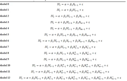
Table 6. OLS Models Description
The table reports the equations of the implied volatility predictive models. These are linear regressions that are used to predict the implied volatility of both the DJII stocks and of the S&P 500 Index.
We use the OLS regressions to forecast the implied volatility using different combinations of the input variables and evaluate their performances. Table 6 illustrates the different models used in this analysis.
To evaluate the OLS models we look both at the IS and OOS. As a main measure of IS performance we use is the computed as
Where SST is the total sum of squares of the dependant variable S and SSR is the Sum of Squared Residuals from the regression.
To evaluate the OOS performance of the models we use two popular error measures, Mean Squared Error and Mean Absolute Error.
These measures are calculated as
Secondly we use the Neural Networks regressions, which are a more flexible type of models when comparing to the OLS model with fewer assumptions for their calculations (Kaastra et al. (1995), Bailey et al. (1990)).
Neural networks are revolutionary models created using artificial intelligence designed to replicate the extraordinary human’s brain capacity to recognize patterns.
Once developed under a scientific background, neural networks have become more and more important in Finance for a variety of applications ranging from economic forecasting to portfolio applications.
Neural Networks are non-linear functions that are a relevant tool for identification of patterns and forecasting according to them. These functions can better incorporate the heavy tails, the noise, the chaos and other non-normality characteristics of the distributions.
In our Neural Networks models we use the backpropagation method which is the most widely used for financial times-series analysis according to Caudill et al. (1992).
The backpropagation is a method where we use connect the inputs to hidden layer neurons and these neurons to the outputs. Neurons are fully interconnected parts of the network that receive and process inputs to produce an output using a transfer function. The main objective of the transfer function is to prevent outputs of reaching extreme numbers that would stop their training. Levich et al. (1993) conclude that this function should be nonlinear and continuous.
As a consequence, the most commonly used transfer function in time series analysis is the Sigmoid S-Shaped function.
The Sigmoid function is computed by:
Where is the scaled input of the neuron, which is obtained by the multiplication of the values of preceding neurons by their respective weights. is the output of a processing neuron.
The architecture is divided in different layers: the input layer, one or more hidden layers and an output layer. The researcher has to determine how many hidden layers and neurons are used in order to build the network architecture. Hecht-Nielsen et al. (1989) shows that three layers are enough to get a good proxy for any continuous function.
The number of input neurons is the number of input variables and the output neuron is the output variable. When we have no hidden layers in the neural network it becomes identical to a linear regression. The weights are the measure of the connection strength between two neurons from different layers. The network adjusts the weights so that it minimizes the sum of squared errors in the estimation. In the end the knowledge of the trained network is then stored in the neurons.
There is no generalized methodology to choose the ideal number of hidden neurons. The choice of too many neurons can lead to over fitting of the data, which means that the network, instead of capturing the patterns, just memorizes the data which may lead to poor out-of-sample performances. Baily et al. (1990) suggest that the number of hidden neurons should be 75% of the number of inputs. Katz (1992) and Klimasauskas (1993) just define a range in which the number of neurons should stand. Accordingly we use two hidden neurons for our models given the reduced number of input variables.
The training is also very relevant for the quality of our network. If we do too many training we might get over fitting on the network. Another problem with the networks is that it may not find the global maximum and may stock in a local maximum. We should define the number of iterations so that increasing the number of iterations would not improve the models significantly.
The market analysis of the S&P 500 implied volatility will be done in an identical way using the same combinations of input variables for each of the models. Given the complexity of the Neural Networks models, our analysis of the DJII stocks focus on the models with the best OOS performance under the OLS framework and the simple model that just account for the lagged volatility so that we can compare the improve in the performance by adding the information flow into the inputs of the model. The two neural networks regressions used will have the same inputs as the model 1 and 4 respectively.
In the end we perform several comparisons of the IS and OOS performances, of the models to better access their relative performances.
All these models are compared with the simple traditional volatility models using the Mean Squared Error and other measures for that purpose. Thus a similar comparison is performed against our models to evaluate their In Sample and their Out-of-Sample performances.
V.
Results
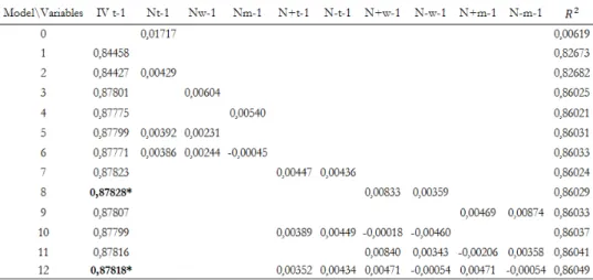
Table 7 shows the results from the In-Sample predictive models for the DJII stocks. First of all, we run two univariate models: one using the number of news and the other using the implied volatility in the previous day. The first model shows very poor IS results shown by a very poor of 0.6%. This happens because, even though we believe that it is a significant variable, it is not by far the only variable that should be taken into account to do such estimation. The model 1 shows good IS results having an of 82,7%, mostly because of the strong autocorrelation of the implied volatility. This autocorrelation is in line with the theory according to which the expectations for the volatility of the following month is strongly correlated with the volatility of the previous month not only due to the volatility persistence addressed by Engle 1982 with the GARCH models. Moreover, the fact that we are using overlapping data strengthens this correlation and thus its significance for the models.
Table 7. In Sample Results from the OLS Regression Models on the DJII stocks
The table reports the betas coefficients of the In-Sample OLS regressions on the DJII stocks implied volatility and the associated with them. * Means that the coefficient is significant with 95% of confidence.
Then we combine both the implied volatility and the lagged number of news in one model. This model does not get any better since the Nt-1
variable has kurtosis too big because of the fact that, in several months, it gets 0 and in others it gets some extreme values.
According to this, we expect to have better results in the models with weekly (Nw-1) and monthly (Nm-1) variables rather than in the daily (Nt-1) ones, since these variables are more uniform with less jumps over time. Indeed, an analysis to the In Sample results indicates the superior results of these models over the daily ones. Table 8 confirms the OOS superiority of these models in predicting the implied volatility (MSE of 0.00057 and 0.00046 in the models 3 and 4 respectively against 0.00086 in model 2).
Table 7. OOS Results from the OLS Regression Models on the DJII Stocks
The table reports the betas coefficients of the OOS OLS regressions on the DJII stocks implied volatility and the R2 associated with them. * means that the coefficient is significant with 95% of confidence.
From the OOS performances we can also conclude that, from the first group of models, the one that shows the best performance is the model 4 (having a MSE of 0.00046) which uses only two independent variables: the IVt-1 and the Nm-1. The superiority of this model may exist not only
Model MSE MAE
0 0,76532 0,07249 1 0,00065 0,01261 2 0,00086 0,01312 3 0,00057 0,01199 4 0,00046 0,01126 5 0,00081 0,01259 6 0,00074 0,01230 7 0,00087 0,01343 8 0,00059 0,01179 9 0,00051 0,01116 10 0,08048 0,00634 11 0,08049 0,00635 12 0,00064 0,01165
the following month, but also the effect of having a smoother and more continuously distributed variable.
Afterwards we take some conclusions on how taking into account the different impact of the news in the previous periods on the returns influence the predictability power of the variables. In other words, we want to see if accounting for the asymmetry of response of volatility to positive news compared to negative news can improve the performance of the volatility models. However, from the Out-of-Sample analysis in table 8 we conclude that the models with the sign variables have inferior OOS performances. Nevertheless we have to take into account that these poor performances might not be related with its explanatory power but rather with the lower degrees of freedom.
We can then conclude that the investors are not influenced just by the most recent news in the recent days to build their expectations but on the overall media coverage in the previous month.
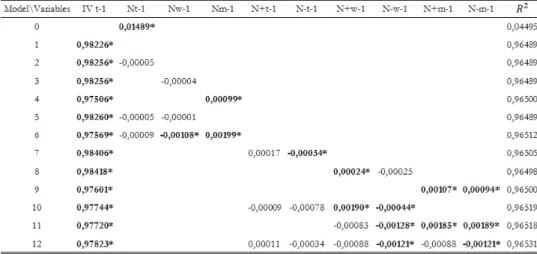
Table 9. In Sample Results from the OLS Regression Models on the S&P 500
The table reports the betas coefficients of the In-Sample OLS regressions on the S&P 500 Index implied volatility and the associated with them. * Means that the coefficient is significant with 95% of confidence.
To perform the analysis of the forecasting model for the S&P implied volatility we follow a similar methodology to the one used for the individual stocks. Table 9 presents the In Sample performance of the OLS regression models at the prediction of the S&P 500 Implied volatility. Similarly to the
results for the Individual stocks, the model that does not consider the lagged implied volatility gets very poor results. In fact, the lagged implied volatility is significant in all the models performed, which shows its relevance for the implied volatility forecasting. Furthermore, as we can see in the table 9, from all the variables we use, the most relevant ones are the ones that include the number of news in the previous month. These variables are significant in almost all the models, which is representative of its significance to forecast the implied volatility, even in models with several variables.
The table reports the betas coefficients of the Out-of-Sample OLS regressions on the S&P 500 implied Volatility and the associated with them. * denotes the significance at 5% significance level.
However, when we analyse table 10 regarding the OOS performance of the S&P 500 models we understand that the best MSE performance is met in model 2, the one that uses the number of news in the previous day. Following this OOS performance analysis, all the models but model 2 are beaten by model 1, that only uses the lagged implied volatility. Furthermore
Table 10. OOS Results from the OLS Regression Models on the S&P 500 Index IV
Model MSE MAE
0 0,005642 0,071864 1 0,000134 0,008109 2 0,000134 0,008106 3 0,000139 0,008205 4 0,000139 0,008166 5 0,000139 0,008202 6 0,000137 0,008054 7 0,000139 0,008221 8 0,000139 0,008229 9 0,000139 0,008170 10 0,000136 0,008060 11 0,000136 0,008067 12 0,000164 0,009092
if we analyse the MAE instead we find that the best results are found in the model 6 that takes into consideration the positive and negative weekly news and that model 2 has the third best performance. This is explained by the fact that this measure gives more weight to the extremes.
Table 11. In-Sample and OOS results from the Neural Network Regressions on the DJII
stocks IV
Model 1 Model 4
IS OOS IS OOS
MSE MAE MSE MAE MSE MAE MSE MAE
Average 0,00124 0,01818 0,00072 0,01737 0,00122 0,01668 0,00065 0,01523 The table reports the Mean Squared Error Measure and Mean Average Error measure from the IS and OOS results from the Neural Networks regressions on the DJII stocks Implied Volatility for all the Models. The Neural Network regressions are two layer neural networks with one output neuron, the Implied Volatility. For the Neural Network regression we use a random data division, apply the Levenberg-Marquardt training rule and use the Sum of Squared Errors as the performance measure.
From table 11 we can conclude that similarly to what we conclude from the OLS regressions, in the neural networks regressions the model with the best performance is clearly model 4, the one that includes the lagged volatility and the average number of news in the previous month. This conclusion reveals the importance of these variables over the others on predicting implied volatility.
Therefore to further study how better a model becomes using this information flow variable in a Neural Network regression, we run the model with that variable and the lagged news and another model with just the implied volatility. Table 11 shows the IS and OOS performances of the model without this variable, model 1, and of model 4 with the information flow of the last month. Model 4 has clearly better performances having and OOS MSE of 0.00065 against an MSE of 0.00072 from the simple model 1.
Table 12. In-Sample and OOS results from the Neural Network Regressions on the S&P
500 index IV
Model\Performance IS OOS
MSE MAE MSE MAE
0 0,022318 0,109034 0,001799 0,018308 1 0,010456 0,075497 0,000881 0,013458 2 0,000350 0,011119 0,000036 0,002074 3 0,000474 0,014854 0,000044 0,002453 4 0,000349 0,011150 0,000036 0,002068 5 0,000459 0,014400 0,000044 0,002445 6 0,000350 0,011218 0,000036 0,002103 7 0,000469 0,014639 0,000042 0,002389 8 0,000481 0,015049 0,000044 0,002501 9 0,008892 0,063229 0,000553 0,010278 10 0,000468 0,014708 0,000044 0,002477 11 0,000472 0,014879 0,000044 0,002452 12 0,022318 0,109034 0,001799 0,018308
The table reports the Mean Squared Error Measure and Mean Average Error measure from the IS and OOS results from the Neural Networks regressions on the S&P 500 index Implied Volatility for all the Models. The Neural Network regressions are two layer neural networks with one output neuron, the Implied Volatility. For the Neural Network regression we use a random data division, apply the Levenberg-Marquardt training rule and use the Sum of Squared Errors as the performance measure.
Table 12 presents the results from the In-Sample and Out-of-Sample neural network regressions on the S&P 500 index implied volatility. Again the model without the lagged implied volatility is clearly outperformed by the other models. However, the model with that just uses the lagged implied volatility is beaten by almost all the models with exempt to the model 12 where the several number of variables used leads to a significant cut in its OOS performance. Similarly to what happens with the DJII regressions, in the S&P neural networks, the model with the best performance is the model 4 (MSE of 0.000036 and MAE of 0,002068). This supports the hypothesis that the average number of news in the financial times is indeed a relevant
VI.
Conclusions
This paper explores the relative importance of the financial media in predicting the implied volatility of stock returns. According to previous literature (Kalev et al. (2004)), the volatility is proportional to the information dissemination rate. We develop measures for the information flow variable based on the amount of news released in the Financial Times. Then, we investigate how the news can improve the implied volatility predicting models using, not only OLS regressions, but also neural network regressions.
We collected data of news, returns and implied volatility from the S&P 500 Index and from all the stocks of the Dow Jones Industrial Average Index from 2004 to 2013. Our results reveal an improved performance of most of the models that include the news in the previous periods. The most relevant variable was the average number of news in the previous month, which makes the model 4 the one with the best performances both at a firm level and at a market level.
Finally, even after controlling for the potential bias in the assumptions of the OLS by using the Neural Networks, we still conclude that the inclusion of the information flow variable related to the number of news released in the previous month strongly improves the IS and OOS performances of our models.
We leave ground for future research to dig into these effects in different markets and using different newspapers as reference. An analysis of the effect of the Financial Times news on the realized volatility forecasting is also expected to produce interesting results. Finally, now that we prove the relevance of the Financial Times news in predicting both the market and the firm specific implied volatility, research could also be done to combine the market risk and the company specific risk into the same variable.
VII.
Appendix
Table 1. Search Queries for each of the 30 stocks in the DJII index
Ticker Name
MMM UN Equity 3M
AXP UN Equity American Express
T UN Equity AT&T
BA UN Equity Boeing
CAT UN Equity Caterpillar
CVX UN Equity Chevron
CSCO UW Equity Cisco Systems
KO UN Equity Coca-Cola
DD UN Equity Dupont
XOM UN Equity Exxon Mobil
GE UN Equity General Electric
GS UN Equity Goldman Sachs Group
HD UN Equity Home Depot
INTC UW Equity Intel
IBM UN Equity IBM
JNJ UN Equity Johnson & Johnson
JPM UN Equity JPMorgan Chase
MCD UN Equity McDonald's
MRK UN Equity Merck
MSFT UW Equity Microsoft
NKE UN Equity NIKE
PFE UN Equity Pfizer
PG UN Equity Procter & Gamble
TRV UN Equity Travelers Cos
UTX UN Equity United Technologies
UNH UN Equity UnitedHealth
VZ UN Equity Verizon Communications
V UN Equity Visa
WMT UN Equity Wal-Mart
DIS UN Equity Walt Disney
The table presents the search queries used in the Javascript and VBA program to scrap all the news from all the stocks in the DJII. The name of the stocks on the right are the text searched on FT.com search bar.
Table 2. Variables Description
IVt-1 Implied Volatility of the options on the underlying
stock using the BS Model
Nt-1 Number of company related news in the previous day
Nw-1 Number of company specific news in the previous
week
Nm-1 Number of company specific news in the previous
month
N+t-1 Number of company related news in the previous day
if the returns were positive
N-t-1 Number of company related news in the previous day
if the returns were negative
N+w-1 Average number of company related news in the
previous week if the returns were positive
N-w-1 Average number of company related news per day in
the previous week if the returns were negative
N+m-1 Average number of company related news per day in
the previous month if the returns were positive
N-m-1 Average number of company related news per day in
Table 6. OLS Models Description Model 0 Model 1 Model 2 Model 3 Model 4 Model 5 Model 6 Model 7 Model 8 Model 9 Model 10 Model 11 Model 12
VIII.
Acknowledgements
Firstly and foremost, I would like to thank the Professor Pramuan Bunkanwanicha for all the support in defining the structure and the directions to take on my research paper. Secondly, I am grateful to Joni Kokkonen for all the guidance provided, feedback and support for my thesis. I would also like to thank Hussein, Martinha and João for the efforts in refining my final dissertation. Thirdly, I would also like to thank my family and friends for always being present. Finally I would like to thank Inês, not only because of her meticulous help but also for her support even in the most stressful periods of the dissertation.
IX.
References
[1] V. Akgiray, “Conditional Heteroscedasticity in Time Series of Stock Returns: Evidence and Forecasts,” The Journal of Business, vol. 62, pp. 55–80, Jan. 1989.
[2] M. Alanyali, H. S. Moat, and T. Preis, “Quantifying the Relationship Between Financial News and the Stock Market,” Sci. Rep., vol. 3, Dec. 2013.
[3] T. G. Andersen, T. Bollerslev, F. X. Diebold, and P. Labys, “Modeling and Forecasting Realized Volatility,” pp. 1–48, Apr. 2006.
[4] T. G. Andersen, “Return Volatility and Trading Volume: An
Information Flow Interpretation ofStochastic Volatility,” The Journal of Finance, vol. 51, pp. 169–204, Mar. 1996.
[5] D. L. Bailey and D. Thompson, “Developing neural-network applications,” AI Expert, vol. 5, no. 9, pp. 34–41, Jun. 1990. [6] T. D. Berry and K. M. Howe, “Public Information Arrival,” The
Journal of Finance, vol. 49, pp. 1331–1346, Oct. 2007.
[7] F. BlackFisher, “Studies of Stock Price Volatility Changes,” American Statistical Association, pp. 177–181, Mar. 1976.
[8] F. Black and M. Scholes, “The Pricing of Options and Corporate Liabilities,” The University of Chicago Press, vol. 81, pp. 637–654, Jun. 1973.
[9] T. J. Brailsford and R. W. Faff, “An evaluation of volatility forecasting techniques,” Journal of Banking & Finance, vol. 20, pp. 419–438, Feb. 1996.
[10] P. A. Braun, D. B. Nelson, and A. M. Sunier, “Good New, Bad News, Volatility, and Betas,” The Journal of Finance, vol. 50, no. 5, pp. 1575– 1603, Dec. 1995.
[11] C. Brooks and G. Persand, “Volatility forecasting for risk
Help?,” Journal of Forecasting, vol. 17, pp. 59–80, Jan. 1998.
[13] J. Y. Campbell and L. Hentschel, “No news is good news,” Journal of Financial Economics, vol. 31, no. 3, pp. 281–318, Jun. 1992.
[14] J. Y. Campbell and Y. Hamao, Predictable Stock Returns in the United States and Japan. 1991.
[15] L. Canina and S. Figlewski, “The Infromational Content of Implied Volatility,” The Review of Financial Studies 1993, vol. 6, pp. 659–681, Oct. 2005.
[16] B. J. Christensen and N. R. Prabhala, “The relation between implied and realized volatility,” Journal of Financial Economics, vol. 50, pp. 125– 150, Oct. 1998.
[17] R. Cont, “Empirical properties of asset returns: stylized facts and statistical issues,” Quantitative Finance, vol. 1, pp. 223–236, Oct. 2000. [18] J.-G. Cousin and T. de Launois, “News Intensity and Conditional Volatility on the French Stock
Market,” ESA, Université de Lille II, France, pp. 1–64, Sep. 2006.
[19] A. F. Darrat, M. Zhong, and L. T. W. Cheng, “Intraday volume and volatility relations with and without public news,” Journal of Banking & Finance, vol. 31, no. 9, pp. 2711–2729, Sep. 2007.
[20] E. Dimson and P. Marsh, “Volatility Forecasting Without Data-Snooping,” Journal of Banking & Finance, pp. 399–421, Nov. 1990. [21] L. H. Ederington and J. H. Lee, “How Markets Process Information:
News Releases and Volatility,” The Journal of Finance, vol. 48, pp. 1161– 1191, Sep. 1993.
[22] R. Engle, “Dynamic Conditional Correlation,” Journal of Business & Economic Statistics, vol. 20, no. 3, pp. 339–350, Jul. 2002.
[23] R. F. Engle and V. K. Ng, “Measuring and Testing the Impact of News on Volatility,” The Journal of Finance, vol. 48, pp. 1749–1778, Dec. 1993.
[24] R. F. Engle and V. K. Ng, “Measuring and Testing the Impact of News on Volatility,” The Journal of Finance, vol. 48, pp. 1749–1778, Dec. 1993.
[25] R. F. Engle, “Autoregressive Conditional Heteroscedasticity with Estimates of the Variance of United Kingdom Inflation,” Econometrica, vol. 50, pp. 989–1007, Jul. 1982.
[26] T. W. Epps and M. L. Epps, “The stochastic dependence of security price changes and transaction volumes: implications for the mixture-of-distributions Hypothesis,” Econometrica, vol. 44, pp. 305–321, Mar. 1975BC.
[27] E. F. Fama, “Efficient Capital Markets A Review of Theory and Empirical Work,” The Journal of Finance, vol. 25, pp. 28–30, May 1979. [28] L. Fang and J. Peress, “Media Coverage and the Cross-Section of
Stock Returns,” pp. 1–45, Oct. 2008.
[29] F. Fernández-Rodriguez, C. González-Martel, and S. Sosvilla-Rivero, “On the profitability of technical trading rules based on artificial neural networks: Evidence from the Madrid stock market,” Economic Letters, pp. 89–94, Mar. 2000.
[30] P. H. Franses and D. Van Dijk, “Forecasting Stock Market Volatility Using (Non-Linear) Garch Models,” Journal of Forecasting, vol. 15, pp. 229–235, Mar. 1996.
[31] M. Frommel, A. Mende, and L. Menkhoff, “Order Flows, News, and Exchange Rate Volatility,” pp. 1–2, Jul. 2007.
[32] J. M. Griffin, N. H. Hirschey, and P. J. Kelly, “How Important Is the Financial Media in Global Markets?,” Review of Financial Studies, vol. 24, no. 12, pp. 3941–3992, Nov. 2011.
[33] P. R. Hansen and A. Lunde, “A forecast comparison of volatility models: does anything beat a GARCH(1,1)?,” J. Appl. Econ., vol. 20, no. 7, pp. 873–889, 2005.
[34] D. Jenter, “Market Timing and Managerial Portfolio Decisions,” pp. 1–47, Jul. 2005.
[35] I. Kaastra and M. Boyd, “Designing a Neural Network for forecasting financial and economic time series,” Neurocomputing, pp. 215–236, Mar. 1995.
[36] P. S. Kalev, W.-M. Liu, P. K. Pham, and E. Jarnecic, “Public
information arrival and volatility of intraday stock returns,” Journal of Banking & Finance, vol. 28, no. 6, pp. 1441–1467, Jun. 2004.
[37] J. O. Katz, “Developing neural network forecasters for trading,” Technical Analysis of Stocks and Commodities, 1992.
[38] S. J. Koopman, B. Jungbacker, and E. Hol, “Forecasting daily variability of the S&P 100 stock index using historical, realised and implied volatility measurements,” Journal of Empirical Finance, vol. 12, no. 3, pp. 445–475, Jun. 2005.
[39] C. G. Lamoureux and W. D. Lastrapes, “Heteroskedasticity in Stock Return Data: Volume versus GARCH Effects,” The Journal of Finance, vol. 45, pp. 221–229, Mar. 1990.
[40] S. S. Lee and P. A. Mykland, “Jumps in Financial Markets: A New Nonparametric Test and Jump Dynamics,” Review of Financial Studies, vol. 21, no. 6, pp. 2535–2563, Oct. 2006.
[41] S. Manzan and F. Westerhoff, “Representativeness of News and Exchange Rate Dynamics,” pp. 1–21, May 2003.
[42] H. Markowitz, “PORTFOLIO SELECTION*,” The Journal of Finance, vol. 7, no. 1, pp. 77–91, Apr. 1952.
[43] M. Martens, “Predicting financial volatility:High-frequency time-series forecasts vis-à-vis implied volatility,” pp. 1–42, Jun. 2002.
[44] R. Matthew and T. Smith, “A Direct Test of the Mixture of
Distributions Hypothesis: Measuring the Daily Flow of Information,” The Journal of Financial and Quantitative Analysis, vol. 29, pp. 101–116, Mar. 1994.
[45] G. McQueen and K. Vorkink, “Whence GARCH? A Preference-Based Explanation for Conditional Volatility,” Review of Financial Studies, vol. 17, no. 4, pp. 915–949, Oct. 2003.
[46] R. C. Merton, Option Pricing when underlying stock returns are discontinuous. 1975.
on the Stock Market,” The Journal of Finance, pp. 1–29, Oct. 2007. [48] M. Mun and R. Brooks, “The roles of news and volatility in stock
market correlations during the global financial crisis,” Emerging Markets Review, vol. 13, no. 1, pp. 1–7, Mar. 2012.
[49] A. R. Pagan and G. W. Schwert, “Alternative Models For Conditional Stock Volatility,” Journal of Econometrics, vol. 45, pp. 267–290, Oct. 1990.
[50] S.-H. Poon and C. W. J. Granger, “Forecasting Volatility in Financial Markets: A Review,” Journal of Economic Literature, vol. XLI, pp. 478– 539, May 2003.
[51] J. M. Poterba and L. H. Summers, “The Persistence of Volatility and Stock Market Fluctuations,” American Economic Review, pp. 1142–1151, Feb. 1987.
[52] S. A. Ross, “Information and Volatility: The No-Arbitrage Martingale Approach to Timing and Resolution Irrelevancy,” The Journal of Finance, vol. 44, pp. 1–17, Mar. 1989.
[53] G. W. Schwert, “Why Does Stock Market Volatility Change Over Time?,” The Journal of Finance, vol. 44, pp. 1115–1153, Dec. 1989. [54] P. Tetlock, “Does Public Financial News Resolve Asymmetric
Information?,” pp. 1–52, Apr. 2010.
[55] L. L. Veldkamp, “Media Frenziesin Markets for Financial Information,” pp. 1–41, May 2004.
[56] K. D. West and D. Cho, “The predictive ability of several models of exchange rate volatility,” Journal of Econometrics, vol. 69, pp. 367–391, Feb. 1995.
[57] G. Zhang, B. E. Patuwo, and M. Y. Hu, “Forecasting with artificial neural networks: The state of the art,” International Journal of Forecasting, pp. 35–62, Jul. 1998.
[58] G. Zumbach, F. Corsi, and A. Trapletti, “Efficient Estimation of Volatility using High Frequency Data,” Research Institute for Applied Economics, pp. 1–22, Feb. 2002.