DEVELOPMENT OF SIMULATION SOFTWARE
AND CALCULUS OF THE AUTOMATED GUIDED
VEHICLES SWEEPS
PEDRO ALEXANDRE MONTEZ OLIVEIRA DUARTE
DISSERTAÇÃO DE MESTRADO APRESENTADA
À FACULDADE DE ENGENHARIA DA UNIVERSIDADE DO PORTO EM ENGENHARIA INDUSTRIAL E GESTÃO
Development of simulation software and calculus of the automated
guided vehicles sweeps at
ASTI (Automatismos y Sistemas de Transporte Interno S.A.U.)
Pedro Alexandre Montez Oliveira Duarte
Master dissertation
Supervisor at FEUP: Prof. Maria Teresa Galvão Dias Supervisor at ASTI: Eng. Jesús Enrique Sierra García
Faculda de de Engenharia da Universidade do Porto Mestrado Integrado em Engenharia Industrial e Gestão
I dedicate this work to the most important people in my life For what they have taught me For the unconditional support For whom I am today
To my parents To my family To my friends
Development of simulation and calculus of the automated guided vehicles sweeps
Abstract
In this era of technology growth, with the appearance of drones, vehicles that park by themselves automatically, submarines that drive autonomous, it starts to feel that the artificial intelligence is overcoming the human one.
The AGVs, automated guided vehicles, are continuosly transforming the industrial enviroment. Althought AGVs is one tecnology that came from the fiftys, it has just started to grow since the 21st century.
AGVs are normally used at industrial levels to transport big loads and/or to perform sequence of repetitive movements. The main functionality is to help companies save time, money and work.
The principal function of the AGVs is to support the factory workers on the hardest tasks such as towing, rising, pushing and forklifting loads, both at the warehouse logistics, internal and external transport as well as supporting the production lines.
These vehicles own an internal software, which controls the AGV movement with the help of sensors and strips. Some of these AGVs can communicate with a central computer to know its position and to receive orders from it, in order to either move or stop depending of the rest of the AGVs.
The purpose of this project is to acquire one software that be able to create routes for the different vehicles of any company, showing the exact sweep of the vehicles and their trailers to the user. It is also importat to avoid collisions with other areas in the factory layout, as well as to generate a precise route in order. This accuracy in the route is crucial, in order to achieve client satisfaction, as well as to facilitate the job of the technicians when they are placing the strip on the clients plant.
Development of simulation and calculus of the automated guided vehicles sweeps
Resumo
Neste período de grande crescimento tecnológico, com o aparecimento de drones, de veículos a estacionar automaticamente, submarinos que se conduzem autonomamente, começa-se a sentir que o período de sobreposição da inteligência artificial face à humana estará cada vez mais próximo.
Os veículos guiados automaticamente têm vindo cada vez mais a transformar o ambiente industrial. Estes veículos normalmente denominados por AGVs, sigla que vem do termo inglês, Automated Guided Vehicles, é uma tecnologia que já vem dos anos 50, mas só a partir do século 21 é que começou realmente a cresçer.
Os AGVs, são especialmente utilizados a nível industrial para movimentar grandes cargas e/ou para fazer sequências de movimentos repetitivos e têm como principal função ajudar as empresas a poupar tempo, dinheiro e trabalho.
A função central dos AGVs é auxiliar os operários da fábrica em tarefas mais complicadas como: rebocar, elevar, empurrar e empilhar cargas, tanto a nível logístico de armazenamento e de transporte a nível interno e externo da fábrica, bem como a nível de auxliar de linhas de produção.
Estes veículos possuem um software interno, o qual com a assistência de sensores e bandas controlam o seu movimento. Por sua vez alguns destes AGVs poderão comunicar com um computador central para conhecerem a sua posição, o qual analisando as diferentes posições dos restantes AGVs indicará a cada um a sequência de tarefas a efectuar.
Este projecto teve como finalidade de adquirir um software capaz de criar rotas para os diversos veículos de uma dada empresa, sabendo exactamente por onde passa cada parte do veículo e seus reboques de modo a evitar zonas de conflito com outras zonas da fábrica, bem como gerar uma rota mais precisa de modo tanto a satisfazer o cliente em questão, bem como de facilitar a tarefa aos operários que têm que representar esta rota no solo de cada fábrica.
Acknowledges
Towards the end of this project, I would like to thank everyone that has helped me through the development.
First I would like to thank to my supervisor at FEUP, Maria Teresa Galvão Dias, for her support and guidance though the entire project.
From ASTI, I would like to thank my supervisor, engineer Jesús Enrique Sierra García, who has provided assistance unconditionally, by sharing a lot of knowledge and provided an excellent environment, during the entire project. Furthermore, thanks to Juan García, Javier Martínez, Víctor Álvarez and Andrés García that always helped me by sharing their knowledge and offer help. Cannot forget to also thank Santiago Lara and Ángel Martín for all the help to adapt to the ASTI informatics system that were needed and support at any kind of problem that was required. And of course to all the personnel of ASTI, that gave me a great support since the first day and guided me and to its kindness and support.
Last but not least, I would like to that to my parents and family to all the support during my entire life and to my good friends, especially to Sara Chan, Marlene Dinis and Filipe Serra for constant support and encouragement.
Also would like to thank ASTI and to University of Porto that supported me financially, so that I could have a good quality of life and work, even outside of my country.
List of contents
1 Introduction ... 8
1.1 Problem objective ... 8
1.2 Project definition ... 8
1.3 Methodological approach ... 8
1.4 The context of the project: ASTI ... 8
1.5 Thesis layout ... 10
2 Literature review ... 11
2.1 Automated guided vehicles ... 11
2.2 Holonomic and nonholomic system ... 27
2.3 Kollmorgen layout designer ... 29
3 Project development... 31
3.1 Comparing programs... 32
3.2 Ackerman and differential wheels ... 34
3.3 The right curvature ... 36
3.4 Error between simulation and real life ... 38
4 Results ... 41
4.1 Creation of vehicles library ... 41
4.2 Creation of manuals and tutorials ... 42
4.3 Creation of paths ... 43
4.4 Creation of simulations ... 44
4.5 Tags and sensor laser ... 44
5 Analysis and Discussion ... 46
6 Conclusions ... 48
7 Future research ... 49
References ... 50
ANEXX A: Software benchmarking parameters ... 51
ANEXX B: Final Program comparison... 53
ANEXX C: Route layout 1 ... 56
ANEXX D: Route layout 2 ... 57
ANEXX E: Gantt diagram ... 58
ANEXX F1: Created vehicles – One unit ... 59
Acronyms
AC – Alternative Current
AGV – Automated Guided Vehicle
ASTI – Automatismos y Sistemas de Transporte Interno CAD – Computer Aided Design
DC – Direct Current
FI – Frequency Inverter FIFO – First In First Out
M – Motor
PLC – Programmable Logic Controller
QR – Quick Response
RFID – Radio Frequency Identification
SIGAT – Sistema Integrado de Gestão da ASTI Tecnisoft SAD – System application designer
VAD – Vehicle Application Designer VDT – Vehicle diagnostic tool
List of figures
Figure 1 - ASTI history ... 9
Figure 2 - Organization chart... 9
Figure 3 - Wired system – adapted from http://www.fernandezantonio.com.ar/documentos%5CDoc%203%20Puentes%20Grua.pdf . 11 Figure 4 - Wired sensor ... 12
Figure 5 - Guided tapes (magnetic and coloured) ... 12
Figure 6 - Magnetic sensor ... 13
Figure 7 - Optical sensor 1 ... 13
Figure 8 - Optical sensor 2 ... 13
Figure 9 - Laser transmitter/ receiver ... 13
Figure 10 - Reflector... 13
Figure 11 - Triangular system example ... 14
Figure 12 - AGV structure ... 15
Figure 13 - Two tier - two motor 1 ... 16
Figure 14 - Two tier - two motor 2 ... 16
Figure 15 - Four tier - four motors ... 16
Figure 16 - Fixed wheel ... 17
Figure 17 - Free wheel ... 17
Figure 18 - Drive wheels ... 17
Figure 19 - Steer/Drive wheel ... 17
Figure 20 - Omnidirectional wheel ... 17
Figure 21 - RFID reader 1 – adapted from http://www.directindustry.com/prod/sick/rfid-reader-writers-integrated-antenna-894-553760.html ... 18
Figure 22 - RFID reader – reading area – adapted from https://www.mysick.com/PDF/Create.aspx?ProductID=77049&Culture=en-US ... 18
Figure 23 - RFID reader 2 ... 19
Figure 24 - Disk tag ... 19
Figure 25 - Cylinder tag ... 19
Figure 26 - ISO card tag ... 19
Figure 30 - Intersection problem ... 21
Figure 31 - Radio ... 21
Figure 32 - Radio antenna ... 21
Figure 33 - Easybot main interface ... 22
Figure 34 - Battery level indicator ... 23
Figure 35 - Battery charging indicator ... 23
Figure 36 - Charging battery ... 23
Figure 37 - Automatic battery charger & transporter platform 1 ... 24
Figure 38 - Automatic battery charger & transporter platform 2 ... 24
Figure 39 - Manual battery changer 1 ... 25
Figure 40 - Manual battery changer 2 ... 25
Figure 41 - Battery charger ... 25
Figure 42 - Pin hook lowered ... 26
Figure 43 - Pin hook raised... 26
Figure 44 - Car being carried by one Easybot standard ... 26
Figure 45 - Easybot coupling unit ... 27
Figure 46 - Easybot carrying a trailer ... 27
Figure 47 - Easybot Basic pin hook... 27
Figure 48 - 2D holonomic movement system ... 28
Figure 49 - Omnidirectional Easybot ... 28
Figure 50 - Positioning of the wheels at the omnidirectional Easybot ... 28
Figure 51 - Kollmorgen communication scheme ... 30
Figure 52 - Tractor transporting wind blade ... 33
Figure 53 - Ackerman condition ... 35
Figure 54 - Easybot Standard ... 35
Figure 55 - Tractor unit ... 36
Figure 56 - Connection from tractor unit to AGV ... 36
Figure 57 - Maximum angle of rotation of tractor unit ... 37
Figure 58 - Distance between axis ... 37
Figure 59 - Minimum radius calculus... 37
Figure 60 - Gadget for the AGV ... 38
Figure 61 - Path draw by the AGV gadget ... 38
Figure 62- Comparing simulation with real trajectory ... 39
Figure 64 - Path draw by the trailer gadget ... 39
Figure 65 - Simulation and real point analysis ... 40
Figure 66 - Easybot bidirectional ... 41
Figure 67 - Autodesk vehicle tracking - ASTI vehicle library ... 42
Figure 68 - Sweep path analysis for the third client 1 ... 43
Figure 69 - Sweep path analysis for the third client 2 ... 43
Figure 70 - Easybot & trailer 3D simulation ... 44
Figure 71 - Autodesk Vehicle tracking 3D simulation – adapted from https://savoycomputing.wordpress.com/2013/06/ ... 44
List of tables
Table 1 - Variation of tension and it´s perform on the motor... 15
Table 2 - Number of wheels on tractor unit ... 16
Table 3 - Type of wheels ... 17
Table 4 - Different types of tags ... 19
Table 5 - Gantt diagram part 1... 31
Table 6 - Simplified program comparison ... 34
Table 7 - Data to calculate minumum radius ... 38
Table 8 - Improvement for each type of project ... 47
1 Introduction
1.1 Problem objective
The main objective of this project was to understand the behaviour of different vehicles cinematic configurations and to develop a software system based on CAD technology to allow the modelling and simulation of different automatic vehicles sweeps along the plant layout, in order to study possible collisions. (Xidias, Nearchou & Aspragathos, 2009)
1.2 Project definition
One of the problems of defining a route in a factory layout is to understand the behaviour of the vehicle that will perform the route. The definition of the route will generate a specific movement of the vehicle and the variation on the speed will generate different kinds of trajectories. In this project it is important to simulate the path that a vehicle will perform in order to check the possible occurrence of collisions and to specify the appropriate speed to perform the movement, especially in the curves.
Although there are countless types of vehicles (Savant Automation, 2014), in this project there will be considered only two types, the simple and the compound vehicles. The simple vehicles are similar to cars, with a motor unit, where the direction of the movement is defined. Compound vehicles are considered as simple vehicles with trailers.
In order to maximize the AGV float efficiency and effectiveness on their transportation tasks, it is very important to design and optimize the plant layout, the routes and to efficiently define the sweep calculus of the AGVs and their trolleys.
1.3 Methodological approach
First, there was the need to study and understand the different types of vehicles and their configurations in order to comprehend their cinematic behaviour.
Next step was to learn about commercial software integrating CAD algorithms along with a variety of parameters that were evaluated and selected. The evaluation was based on the simulation of one vehicle and its trolleys sweeps along an established route. It was selected a group of vehicles that would be simulated in the chosen program. In the end the selected software was tested with a group of different vehicles and its trolleys. In the end, the improvements achieved by the program were studied.
1.4 The context of the project: ASTI
ASTI is a family company from Burgos, founded in 1982 and dedicated to the study of internal logistics engineering solutions (ASTI, 2014).
The company is constituted by more than 80% of engineers and high qualified technical personnel. The activities of ASTI are of a great variety, from the problem analysis in
The vision of ASTI is “Ser un Referente Mundial, en el suministro de soluciones de automatización y sistematización de logística interna”, which means, to be a world reference in the implementation of automated and systematized solutions of internal logistics.
Figure 1 - ASTI history
So if we analyse this company history, it can be seen that the first generation had one idea of creating a good company since 1982. The new generation in addition to that, wants the internationalization of the company. As it is shown at 2008, they open a commercial office at Argentina and the website also helps in this internationalization (2009). From the timeline it is also notable the amount of awards that the company have received so far.
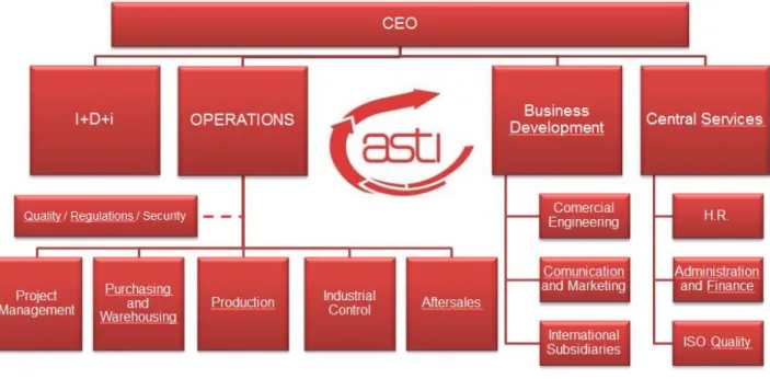
Figure 2 - Organization chart
In the Figure 2, it’s the organization chart of the company ASTI. This project was developed at I+D+i (Investigation, Development and Innovation) department.
1.5 Thesis layout
This thesis is divided in the following main chapters: Introduction:
In this section it is defined the problem objective of this project, what the project consisted and how it was approached. It was also given a brief presentation of the company where the project took place.
Literature review:
This part of the project consisted in the studies realized prior the development of the project. The main features that are explained, is the composition and how works an AGV, analyzing which type of vehicles can be simulated and in the end, the explanation of the previous software program that the company owns.
Project development:
The project development, as it name says, it is the section where is explained all the process for develop this project, in order to be able to produce results for the project.
Results:
At the results section, it is explained the data, documentation and features created for the company.
Analysis and Discussion:
This section is all about the advantages and disadvantages of the project. Showing how it improves project development of the company.
Conclusions:
The conclusions of this project are explained in this section. In here it is analyzed the entire project and what it was achieved with it.
Future research:
In the last chapter of this thesis, it is explained some of the extra features that can be created in order to improve the project at the company.
2 Literature review
2.1 Automated guided vehicles
The base of this project is the study of sweeps of automated guided vehicles, also known as AGVs (Berman, Schechtman, & Edan, 2008). This type of vehicles appeared in 1953 as Savant Automation (2014) explains.
Let´s explain first what is an AGV, how does it work and why it is important to study its sweeps.
In simple terms, an AGV is a vehicle that is automatically driven by itself without the necessity of human interaction. Since human interaction is not required, a group of sensors to drive through the plant of the factory is essential (Savant Automation, 2011). There are several ways to the vehicle to control the direction in an AGV, below is the list of the most common ones:
Wired Guide tape
o Magnetic o Coloured Laser target navigation
Dual (Magnetic guide tape & Laser target navigation)
According to the layout, the wired system is placed on the floor, which serves as a trajectory for the AGV to follow. This wire will transmit a radio frequency (magnetic field) to the sensor installed at the bottom of the AGV and the AGV will follow the wire signal.
Figure 3 - Wired system – adapted from
http://www.fernandezantonio.com.ar/documentos%5CDoc%203%20Puentes%20Grua. pdf
The wired systems have some positive and negative features. The chance of system damage is low due to the installation location, which is underneath the floor. On the other hand, there is difficulty in editing the route and the cost is high.
Figure 4 - Wired sensor
Referring to Figure 4, the wired sensor can follow 8 different frequencies (f1-f8), in this case: 5.1; 5.7; 6.3; 7.0; 7.8; 9.0; 10.0 and 12.0 kHz.
There are two types of guided tapes as shown above: magnetic or coloured. Both of them are placed on the top of the floor, which would make it easier to place and edit, but at same time easier to get damaged. Both tapes are indicated in Figure 5. The blue arrow points to the magnetic tape, and the red one to the coloured one. As you can see in the coloured one, a white and a black tape were utilized to, provide an easier job for the optical sensor to follow the white tape.
Figure 5 - Guided tapes (magnetic and coloured)
Figure 6 - Magnetic sensor
Figure 7 - Optical sensor 1 Figure 8 - Optical sensor 2
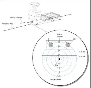
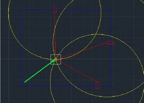
In the laser target navigation we equip the AGV with a rotating laser (transmitter and receiver) which is mounted in a turret. We fix some reflectors around the factory normally at walls and columns, and by triangulating the signal the position of the AGV could be identified. The AGV have a map of all the targets in its internal memory. The usage of the map is to correct its position error.
Figure 11 - Triangular system example
According to Figure 11, we could see an example of how the triangular system works in an AGV. The white square represents the AGV whereas the blue one represents the walls of the factory. The red rectangles represent the reflectors, and the red lines represent the laser that comes out of the laser transmitter/receiver of the AGV. So by knowing the distance from each reflector to the AGV, we could make three circles around each reflector to indicate the joining point. The joining point of the three circles indicates the position of the AGV.
Furthermore, there are other ways of location indication for the vehicle. Inertial (Gyroscopic) navigation
Magnets
Optical camera (QR codification on the roof) Optical reflector (Floor)
The inertial (Gyroscopic) navigation is not yet in use. The magnets, optical camera (QR codification on the roof), and optical reflector (Floor) had been used in the past, however, the accuracy is low.
Now that we understand how an AGV navigates, let´s explain the rest of an AGV. Please see the diagram in Figure 12 for an easier and better understanding of the AGV.
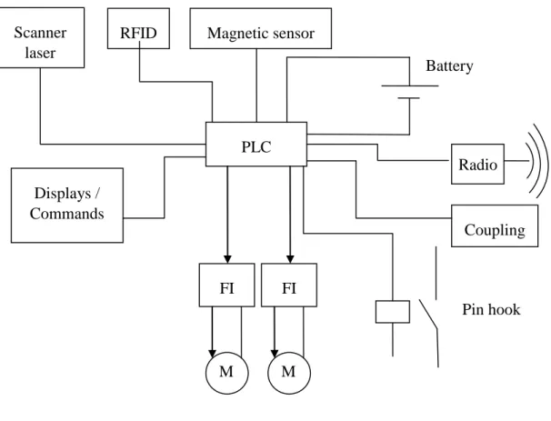
Figure 12 - AGV structure
The PLC (programmable logic controller) is the brain of the AGV. All control functions come from the PLC, which are defined by the users and the AGV must perform.
From the PLC goes tension to the frequency inverter (FI), depending of the tension it performs different types of movement. The necessity of having this component is because the tension from PLC is direct current (DC) and the motor can only receive alternative current (AC).
In Table 1 is an example of how it performs.
Table 1 - Variation of tension and it´s perform on the motor
0V 0-2.5V 2.5V 2.5-5V 5V
Full speed backwards
Variation from stop to full speed
backwards
Motor stops Variation from stop to full speed forwards
Full speed forwards
There is a frequency inverter for each motor. Nevertheless, if the two motors perform the same movement at the same time, the frequency inverter for both motors would be the same. This happens for example in the case below.
PLC FI FI M M Magnetic sensor RFID Radio Battery Scanner laser Pin hook Displays / Commands Coupling
Figure 13 - Two tier - two motor 1
Figure 14 - Two tier - two motor 2
Figure 15 - Four tier - four motors
Figure 15 shows one motor for each wheel, due to the insufficient space for a unique and bigger motor for both wheels.
So far we know that we have one frequency inverter for each side and in each side we can have one or two wheels. This decision to have two or four wheels is just a question about how much power the AGV can carry.
Table 2 - Number of wheels on tractor unit
Number of wheels 2 4
Power able to carry (N) 250 400
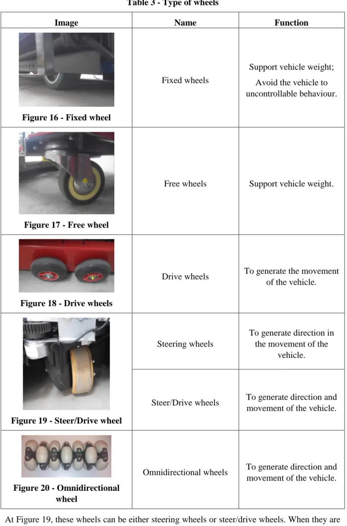
Please note that a vehicle can have different types of wheels, and that they can have different placements. First let´s analyse the type of wheels that a vehicle can have and what are its function.
Table 3 - Type of wheels
Image Name Function
Figure 16 - Fixed wheel
Fixed wheels
Support vehicle weight; Avoid the vehicle to uncontrollable behaviour.
Figure 17 - Free wheel
Free wheels Support vehicle weight.
Figure 18 - Drive wheels
Drive wheels To generate the movement of the vehicle.
Figure 19 - Steer/Drive wheel
Steering wheels
To generate direction in the movement of the
vehicle.
Steer/Drive wheels To generate direction and movement of the vehicle.
Figure 20 - Omnidirectional wheel
Omnidirectional wheels To generate direction and movement of the vehicle.
Until now we have already known what generates the movement of the AGV and how the route is directed. Now let´s see how an AGV knows what to do in each position.
There are two types of systems: RFID system
Information system via wireless to a computer
The RFID system, also known as radio-frequency identification, is a method that identifies an item using radio waves. The basic function of this system is that the vehicle has one RFID reader that will read RFID tags. These tags have some digital information that will be transmitted to the RFID reader and from this to the AGV. There are a big variety of RFID readers and tags. (RFID Journal, 2008)
Basically we have an RFID reader that reads tags along the path. Each tag gives information to the AGV regarding the tasks, such as:
Stop
Move at a certain velocity Raise or lower the pin hook Communicate with computer
o Check if an AGV could move or wait for other AGV moves o Send notification upon arrival at a selected position
Check the battery to see if it need to charge Scanner area
Figure 21 - RFID reader 1 – adapted from
http://www.directindustry.com/prod/sick/rfid- reader-writers-integrated-antenna-894-553760.html
Figure 22 - RFID reader – reading area – adapted from
https://www.mysick.com/PDF/Create.aspx ?ProductID=77049&Culture=en-US In Figure 22, since the tags are placed on the floor and the RFID reader does not have a big altitude to read the tag, they are placed in the bottom of the AGV; please refer to Figure 23.
Figure 23 - RFID reader 2
There are a big variety of RFID tags. The tags are placed on the floor in the positions where the RFID reader on the AGV passes by. In the Table 4 there is an example list.
Table 4 - Different types of tags
Image Model
name Measures Advantages Disadvantages
Figure 24 - Disk tag
Disk
transponder
Radius=30mm Depth=1mm
Easy to change position;
Can be fixed Can be damaged
Figure 25 - Cylinder tag
Cylinder transponder Radius=20mm Depth=5.7mm Protected Small area of radio; Fixed position
Figure 26 - ISO card tag
ISO CARD transponder
Dimensions= 55x85mmm Depth=1mm
Big area of radio; Easy to change position
Very big
dimensions, easy to be damaged
Figure 27 - Coin tag
Coin transponder
Radius =50mm Depth=1mm
Easy to change position; Adhesive surface (to fix on the floor)
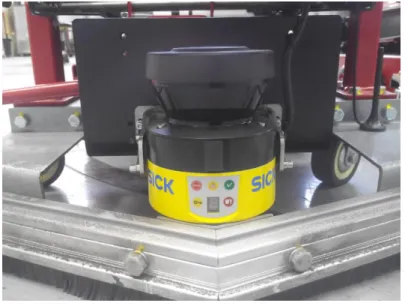
Whenever there is the necessity to a precise stop of the AGV, for example in the case of the AGV stops at an exactly position, instead of using a tag to make the AGV stop, it´s better to add a laser to the AGV. When the AGV arrives to the workstation, there will be a reflector in there, when the laser of the AGV sends and receives the signal transmitted to the reflector, the AGV will perform the precise stop needed, which it can’t be acquired when we use tags. Another important thing to have in the AGV is the scanner laser. Its function is to scan the area around the AGV, so it doesn’t collide with any object, wall or human being. They are normally inserted in front of the direction of the movement, so they can scan the area in front of them to make sure that the vehicle will not collide. As we saw before, the scanner area can be changed during the circuit when the RFID reader scans a tag. (SICK, 2014)
Figure 28 - Scanner laser This area must change in two cases:
Entering a corner; Entering a workstation
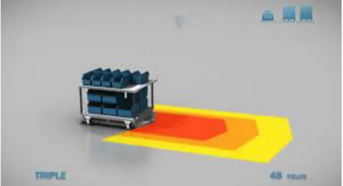
Entering the corner the laser must also see the inside of the corner, and when entering a workstation it must change the area so the AGV does not stop by detecting the workstation. This scanner laser from Sick has 3 different zones, one for security and two for information. The security zone is the smaller area and it´s to stop the vehicle if the scanner scans some “intruder”. The information area 1 is a bit bigger than the security one and it´s used to slower the AGV. The second information area is used to transmit a sound signal to the object that he finds. Please see Figure 29 for better understanding of this.
Figure 29 - Scanner laser areas 1 – adapted from https://www.youtube.com/watch?v=Lubzfam-ouk
Red area - Security zone
Orange area - Information area 1
Yellow area - Information area 2
Now let´s talk about the radio, the function of the radio it´s to communicate with the central computer. This communication is used for example when there are two AGVs and their route crosses one another, like Figure 30. To decide which AGV goes first, normally it´s decided as the FIFO method, (first in first out) and for that it asks the computer which one has permission to move first. (Klimn, Gawrilow, Möhting, & Stenzel, 2008)
Figure 30 - Intersection problem
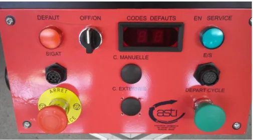
The display/commands it´s where we have the human machine interface. Let´s analyse one vehicle for example, the ASTI Easybot standard. In this vehicle we have 3 human machine interfaces. First we have the main interface: Figure 33.
Figure 33 - Easybot main interface In the main interface we have:
Turn on/off selector (OFF/ON) Display codes (CODES DEFAULTS)
o Errors;
o Readings from sensors; o Movements;
o Communications; Start button
Emergency stop button Display lights
o Working o Error
SIGAT – transfer code to the AGV
Manual control (C. MANUELLE) – manually control the AGV Entry/Exist (E/S) – add extra displays or commands to the AGV External commands (C.EXTERNES)
Other displays that we have are the battery level and a charger indicator.
Figure 34 - Battery level indicator Figure 35 - Battery charging indicator The battery level indicator just works when the AGV is turned on and informs the user about the level of the battery.
To charge the battery it is needed to unplug the battery from the AGV. By doing this we cannot check the battery level indicator and for that reason, is used the Battery charging indicator. The Battery charging indicator will show up to three colours. It will show a red colour when the battery is low and the charging is starting. A yellow light will be displayed when the battery level reached 80%. And it will turn green when the batteries are fully charged.
Figure 36 - Charging battery
The batteries are what give the energy to the AGV to perform all its tasks. The AGVs can work at least 8 hours, some can work 16 hours without charging, all depends on the size, work, speed and carry weight that the AGV is forced to.
For this reason, if we have a factory that works 24h/day we need to have some way to change the battery of the AGVs. In some AGVs we can have the possibility to do it automatically, but in other cases we need to do it manually.
In the automatic mode the AGV position itself next to the interchanger, an electromagnet gets the battery and places it in a platform. The interchanger moves itself to be able to insert the charged battery on the AGV and with the help of an electromagnet it places on the AGV. After this, the platform will move to the charging platform and insert there the uncharged battery so it can be charged. At Figure 37 we have the 8 battery chargers and in front of it we have the transporter platform.
Figure 37 - Automatic battery charger & transporter platform 1
Figure 38 - Automatic battery charger & transporter platform 2
At Figure 38 we can see the wheels that move the transporter platform and the two electromagnets, one of the platform will carry the charged battery and the other the uncharged one.
Other AGVs, which do not have this possibility to have the automatic interchanger of battery, the personnel will have to do it manually, for that there are some battery trolleys. In the Figure
Figure 39 - Manual battery changer 1 Figure 40 - Manual battery changer 2 In these cases the personnel needs to move the battery to a spot where there is the battery charger.
Note: this charger can be inserted inside of the AGV, if there is no need to the AGV to be always running, in other words, if it can be stopped to be charging. In both cases it’s the same charger and it is shown at Figure 41.
Figure 41 - Battery charger
The connection of cars and trailers in an AGV is one of the parts that were important for the study in this project. Please note that not all AGVs can take cars and trailers, some just have a pair of forks and carry pallets. In other cases we have some AGVs that are omnidirectional that basically is a platform that can move in any direction.
Some AGVs can take both cars and trailers, in this project it was studied the Easybot Standard that have this possibility, other vehicles can just carry trailers, what was the case of the Easybot Basic.
The Easybot Standard has a pin hook in the front of it and a coupling in the back. The pin hook in this vehicle is used to transport cars and the coupling unit is to transport the trailer. This AGV has one relay that is connected to a motor and this to a worm screw that will perform the mechanical action of raising and lowering the pin hook.
Figure 42 - Pin hook lowered Figure 43 - Pin hook raised
The black cylinder is the motor, and below it is the worm screw, the grey cylinder. When the pin hook roses it is able to connect with the car. The car can have its wheels in two different types:
All wheels free and connected in the pin hook and at other two points in the AGV All free wheels and two fixed wheels in the same line where the AGV have the fixed
wheels
By doing this, the car and the AGV will have the same behavior in the movement and because of that it can be consider as a bigger AGV, as seen at Figure 44.
Figure 44 - Car being carried by one Easybot standard
Now to carry a trailer, the Easybot Standard has one coupling unit in the back of it. This coupling unit has a fixed position, as shown at Figure 45.
Figure 45 - Easybot coupling unit Figure 46 - Easybot carrying a trailer
In an Easybot Basic there is just a pin hook in the back, meaning that only a trailer can be coupled.
Figure 47 - Easybot Basic pin hook
This pin hook has two ways to connect with the trailer, in Figure 47 it can raise and connect in the top. If we change the screw to the top whole, it can connect in the bottom like an Easybot Standard.
2.2 Holonomic and nonholomic system
When we speak about AGV sweeps, we are not talking about what an AGV does when we give it a brush. What we mean is the study of the movement of each points of the vehicle when it describes one trajectory. Now this calculus can be made with different applications, but until we arrive to them, there have been a lot of historical steps. Let´s start from the beginning.
One AGV behaves in a similar way as a car; in fact both of them belong to the group of a nonholonomic system. For better understand this, let´s explain what a holonomic system is. If we consider a solid, that all the connections of its particles are strong and when this object moves, all the particles inside of the object does not change its position internally like an omnidirectional vehicle, we are talking about a holonomic system. This vehicle is holonomic because the controllable degrees of freedom of it are equal to the total degrees of freedom; in
a two dimensional space we have three degrees of freedom, axis x, y and the rotation on the origin; this type of vehicles have this same behaviour.
On this vehicle the wheels can slide while the others rotate, so we can move in the three degrees of freedom, as it is shown in the Figure 48.
Figure 48 - 2D holonomic movement system
The ASTI Company has this type of vehicles and they name it as omnidirectional Easybot. These types of vehicles have a specific type of wheels not like the conventional one, which will allow doing all this types of movement. In the Figure 49 is an example of it.
Figure 49 - Omnidirectional Easybot
These vehicles have their wheels placed as shown at Figure 50 and the configuration of the wheels is displayed at Figure 20.
But now going back to the example of a car or a tricycle, we do not have this type of behaviour, the components of the vehicle they move inside of the vehicle. For example when we perform a parallel parking on these vehicles, the front wheels move inside the vehicle. The entire vehicle components will perform different type of movements, internally, when it is not moving on a line.
2.3 Kollmorgen layout designer
The first software program used was Kollmorgen layout designer. This software is just used by some types of vehicles, vehicles that use the Kollmorgen information system, but not all vehicles have this information system.
At ASTI, vehicles that used this software were called RoboFast. These vehicles were acquired by the company to an external provider and then the company transform these vehicles into full automated vehicles using Kollmorgen software programs. In additional it will also be added sensor lasers and laser transmitter/receiver for example.
If this software does all of this, why do not we used it to calculate the vehicle sweeps of all the AGVs of the company? The main reason for this is because this software is not able to calculate vehicles with trailers and it is not able to run in a CAD system, which is the common software used to draw the client layout factories.
The layout designer, it’s just one of the programs of the Kollmorgen and its function is to create the sweep paths of vehicles and check if they can have collisions or not with any structure at the factory. But in this program you cannot define the vehicle dimensions, for that you need VAD (vehicle application designer), which is a program that is made just for defining the vehicles.
Another software of Kollmorgen also used is the CWAY, which checks in real time where the vehicle is and shows two distinct colours to see if the vehicle is running well (green colour) or if the vehicle is broken (red colour).
All this programs communicate with each other, and they aren´t the only these ones used, but for this project these are the ones that matter the most.
Figure 51 - Kollmorgen communication scheme
Now it will be explained a bit about the software programs that are represented in the Figure 51.
VAD - Vehicle Application Designer
OPEN PCS - Program the AGV
Layout designer - To draw the route
Reflector surveyor - To place the reflectors position
System Manager - Controls the orders of the AGVs
SAD - System application designer
- To define the task to do in each position
CWAY - Controls in real time the AGVs (human interface)
VDT - Vehicle diagnostic tool
- To analyse the black box of the AGV
Analysing layout designer, it is a software that needs integration with other software programs. It cannot represent the sweeps of most of the company vehicles; we cannot add laser fields and predict where we have to place the tags. It is impossible to represent the
Layout designer SAD System Manager CWAY VDT Reflector Surveyor VAD OPEN PCS
3 Project development
This project was developed at ASTI, for a period of 4.5 months. Table 5 shows the Gantt diagram with each task and its duration.
Table 5 - Gantt diagram part 1 Task
nº Task Duration Beginning End Preceding
1 Project presentation 5days 10/02/2014 14/02/2014
2 Study of layout designer 5days 10/02/2014 14/02/2014
3 Study of system requirements 5days 10/02/2014 14/02/2014 4 Study of market solutions (Inventor,
Autopath, Autoturn…)
5days 17/02/2014 21/02/2014 1, 2, 3
5 Search in the internet of market solutions
5days 24/02/2014 28/02/2014 4
6 Definition of project specifications 5days 24/02/2014 28/02/2014 4 7 Presentation of the project to the
department managers
5days 03/03/2014 07/03/2014 5, 6
8 Parameterization of the EASYBOT vehicle
5days 10/03/2014 14/03/2014 7 9 Test of vehicle sweeps and simulations
with the chosen tool
5days 17/03/2014 21/03/2014 8
10 Parameterization of a trailer connected with an EASYBOT
5days 24/03/2014 28/03/2014 9
11 Parameterization of the different points inside of an EASYBOT vehicle and its laser field
5days 31/03/2014 04/04/2014 10
12 Documentation of the project development
5days 07/04/2014 11/04/2014 11
13 Presentation to the department managers 5days 07/04/2014 11/04/2014 11
14 Holidays 5days 14/04/2014 18/04/2014 12,13
15 Corrections on the program 5days 21/04/2014 25/04/2014 14
16 Parameterization of different vehicles and trailers
15days 21/04/2014 13/06/2014 14 17 Presentation to the CEO and department
managers
5days 12/05/2014 16/05/2014 16
19 Project documentation 15days 26/05/2014 13/06/2014 20 Presentation to the department managers 5days 09/06/2014 13/06/2014
21 Corrections, final adjustments 10days 16/06/2014 27/06/2014 18, 19, 20 22 Formation to the ASTI team 5days 16/06/2014 20/06/2014 18, 19, 20 23 Final presentation with the results to the
department managers
5days 23/06/2014 27/06/2014 22
In Annex E it can be viewed the full Gantt diagram.
The first period at ASTI was devoted to the study of the systems that ASTI uses, and to understand how they could be improved. Since the period of task number 4, it started the investigation of a new CAD software to simulate the sweep path of the vehicles that were not able to perform in the Kollmorgen software.
At task number 7 the best programs were selected and it started the testing of them, in order to understand which one was the best for the company. After selecting the best program it was important was to create as much vehicles as possible, so that ASTI would be able to easily select a vehicle and perform its sweep path analysis. After the creation of these vehicles it was also important to add specific points or areas in the vehicle. These points and areas were then used to simulate the path that the sensor laser would do, and to simulate where to place the tags in order that the RFID reader could read them. These were all extra features added to the software because they were important studies, and were not possible to be performed in the existing program prior the Autodesk Vehicle tracking.
After all of this, there was the necessity to create some documentation and videos in order to support ASTI users of this new software program. By doing these manuals, step by step, it was achieved one big step, reducing the execution time of any task with the program. These tasks consisted of creating a vehicle, placing tags in a route, defining a laser area until the real objective of this project and creating a sweep path analysis of the vehicles.
3.1 Comparing programs
Since there is the need to predict the path of a vehicle, there is a continuous development of software on this field. This kind of programs are starting to be used in the most distinct areas, such as the road vehicles, like cars, tractors with big trailers for example the ones that transport wind blades, or even airplanes. This kind of studies are important mostly for engineers, designers and planners at government agencies and engineering consulting firms to simulate the vehicles movement.
Figure 52 - Tractor transporting wind blade
By predicting the movement of a vehicle, we can reduce the risk of collision, check if a vehicle will be able to perform a certain route or even edit our layout so the vehicle can do a specific route.
There are only quite a few developers of this type of programs, and some design companies are starting to acquire this software and use them as plugins on their main programs like Autodesk.
Some of these software programs were studied, taking into account the most important parameters for the company. In Annex A the list of the most important parameters for this project are presented.
A search on the web, allowed to create a list of some available programs that were studied and compared:
Autodesk vehicle tracking; AutoTurn 2D; AutoTurn 3D; Invision; Malz++Kassner; AutoTrack; Path Planner;
AutoTrack and Path Planner were automatically removed from the comparison, since the first one was acquired by Autodesk and was transformed in the Autodesk vehicle tracking, and the other one, Path Planner, was removed from the market since January 29, 2014.
Malz++Kassner is a German software and one of the main issues using this program, was the difficulty to work with it added to the fact that it was not compatible with the AutoCAD format. Hence, it was decided to leave this program out from our comparison.
In the end, we made a full comparison of the rest of the programs. The main difference between AutoTurn 2D and 3D was the fact that in the 3D we could create 3D vehicles and perform vertical analysis, which were not available on the 2D version.
In the Autodesk vehicle tracking we have everything that AutoTurn 3D and Invision have and we can better define the mechanical characteristics of the vehicle, so it would simulate better the cinematic performance of the vehicle, which will create a better sweep path simulation. In Table 6 it is presented a simplified list of the comparison, at Annex B we can see the full comparison.
Table 6 - Simplified program comparison
Even if in Autodesk vehicle tracking we have an annual cost and AutoTurn 3D it just needs one license without time limit, after comparing both software programs, we decided to go with Autodesk vehicle tracking since it gives a better precision, and it is a very important factor when calculating the sweeps of the vehicles.
3.2 Ackerman and differential wheels
All the software programs that were tested used vehicles with Ackerman wheels; these are the wheels that are used by cars. At this type of movement the vehicle inner wheel will have a bigger inclination then the outer wheel.
The Ackerman condition says: “To have all wheels turning freely on a curved road, the
normal line to the center of each tire-plane must intersect at a common point.” as it is shown
Figure 53 - Ackerman condition
If the vehicles at the Autodesk vehicle tracking have this type of movement and, in the other hand, the vehicles that we could not create on Kollmorgen are differential vehicles; we have to adapt those vehicles to Ackerman’s.
Let´s see the example of the Easybot Standard. An image of one of these vehicles is displayed in the Figure 54.
Figure 54 - Easybot Standard
As we can see in the Figure 54, the AGV have 6 wheels. From front to back, we first have two free wheels, then we have two differential wheels and in the back a pair of fixed wheels. The function of the free wheels is just to support the weight of the AGV, so we just take into account the differential wheels and the fixed ones.
The differential wheels have one motor for each wheel, with two functions, to steer and drive. This vehicle as you can see, have a red metal box that connects these differential wheels to the rest of the AGV. So, basically this red box is the tractor unit of the AGV and we can consider the rest of the AGV as a trailer. Later, it will be explained why we made this analogy. when the AGV wants to perform a perfect line, it will give the same tension to the differential wheels, always taking into account if the following sensor (in this case the magnetic sensor) is following well the stripe on the floor (for a magnetic sensor we have a magnetic stripe). If the magnetic sensor starts to going out of the line, it means the vehicle is entering a curve line, so
be always adjusting while it is in the corner, until it finds a straight line again and will give the same tension to both wheels.
As it can be seen, we have a completely different way to drive an Ackerman vehicle and a differential one. In order to surpass this obstacle, since the software only accepts Ackerman vehicles as tractor units, we considered the vehicle as made in two parts. of the first part is the tractor unit. Even if in the real life we only have 2 wheels in the Autodesk vehicle tracking we must have the 4 wheels, two directional and two fixed, so we made a tractor unit with 4 wheels with the width distance equal to the real life one (of the differential wheels) for both front and back wheels. Then the distance of front and back wheels were joined together so we just have the same behaviour as we had two differential wheels.
To create the rest of the AGV, we consider it as a trailer that was connected at the center of the axis of the tractor unit, and actually it is what occurs in the real life vehicle, even if we consider it as one vehicle with just one part. Figure 55 and Figure 56 represent it.
Figure 55 - Tractor unit Figure 56 - Connection from tractor unit to AGV
3.3 The right curvature
After the adjustment of the AGV to an Ackerman vehicle, it was started the simulation of the AGV in the program. It was discovered that the simulated vehicle was not able to perform the same curves performed by the real vehicle. In an analysis to the simulated vehicle, the problem was found. The tractor unit created has the two front and back axis together and it was not accepted as a mechanical possibility. So, it was studied the minimum curve that the real AGV could perform.
As shown at Figure 57, we calculated the maximum real angle that the vehicle was able to do and its value was 45o for each side. And by knowing the distance between axes (Figure 58), we were able to determine the center of rotation and the minimum radius.
Figure 59 - Minimum radius calculus
As we can see in Figure 59, we were able to determine the minimum radius of curvature from here. After editing the distance between axes of the tractor unit, we achieved the distance that we needed to perform the minimum radius curvature and with this we had our vehicle fully simulated.
Figure 57 - Maximum angle of rotation of tractor unit
Figure 58 - Distance between axis
45º 45º Dist anc e be tw ee n a xis Minimum radius
Table 7 - Data to calculate minumum radius
Angle Distance between axis Minimum radius
45º 795mm 1124.3mm
3.4 Error between simulation and real life
After the full specification of the vehicle, there was the need to check the error between the real movement of the vehicle and the trajectory simulated in the software application.
We created a gadget to add to the vehicle and its trailer. This gadget was composed by some metal plates, steel tubes and screws, and by adding it to the vehicle and inserting one chalk in the tube with a steel cylinder to add some weight to it, the gadget draw the trajectory of one point of the vehicle.
Then we also added the same point to the simulated vehicle and made the simulated vehicle to follow the same path that the real vehicle performed.
Figure 60 and Figure 61 show the gadget that was created and where it was placed.
Figure 62- Comparing simulation with real trajectory
As it can be seen in the Figure 62, the purple line is the simulated line of the gadget and the yellow line is the real trajectory.
For the trailer, there was the necessity to adapt the gadget and it was inserted into two parts of the trailer, one on the left and the other on the right side of it. In the Figure 63 and Figure 64 it is shown the adapted gadget and the insertion of it in one side of the trailer.
Figure 63 - Gadget for the trailer unit Figure 64 - Path draw by the trailer gadget
Figure 65 - Simulation and real point analysis
In Figure 65 we can see in the purple lines the trajectory done by the simulator, and the yellow dots represent where the chalk has passed in the real movement.
By calculating the error distance from simulation in relation to the real life, the biggest error was of 3cm what was very satisfactory, because it demonstrates a great precision.
4 Results
4.1 Creation of vehicles library
Since there is not a single AGV produced at ASTI, there was the necessity to create a list of vehicles, as big as possible, so we could simulate the paths for any vehicle. By measuring the vehicle dimensions and its behaviours, we were able to create almost all type of vehicles that the company produced, but some of those vehicles were not able to be used in simulation due to its strange configuration.
The vehicles that were not possible to create in the software were the Easybot bidirectional, Easybot omnidirectional and the Quad vehicle.
Let´s explain why these vehicles were not able to be simulated in the software.
The bidirectional was not possible to be used in the Autodesk vehicle tracking, because it is an AGV with two different tractor units.
Figure 66 - Easybot bidirectional
As it can be seen at Figure 66, this vehicle have two tractor units, both of them follow the magnetic stripe. Since the same vehicle has two tractor units it does not move as the normal vehicles, like a car that only has one tractor unit. Since the vehicle has this behaviour it cannot be simulated as normal car, because this vehicle can do hardest curves that the normal vehicle cannot.
Now let´s examine both Quad and Easybot omnidirectional. The problem of these vehicles in the simulation is that they are holonomic. As it was explained before, this vehicle can move in any directions and rotate by its center and that it is impossible to simulate in a normal car. These are the reasons why these three vehicles cannot be simulated on the Autodesk vehicle tracking.
Even that these three vehicles cannot be simulated, all others can. In the Figure 67 it is the list of vehicles created in the Autodesk vehicle tracking.
Figure 67 - Autodesk vehicle tracking - ASTI vehicle library
Mainly there are two big classes of vehicles at ASTI, the Easybot and the RoboFast. The Easybot are vehicles that are fully developed by the company from its body layout to the programming. The RoboFast are vehicles that the company acquired and use Kollmorgen programs to program the vehicle.
In the list above, Figure 67, all Easybot start with EASYBOT name and then is specific characteristics. And the RoboFast have its first specific name first and then its characteristics. Both types of vehicles have characteristics that never change so and those are not specified on the name.
4.2 Creation of manuals and tutorials
During the project it was developed some documentation and videos, in order to support the Autodesk vehicle tracking users. The documentation consisted in two manuals; one of them is mainly about vehicle configuration and the other one about creating trajectories. The reason for creating two manuals instead of just one was by taking into account the final user of it; some users in the company will create vehicles, the mechanical department and the other users will be from the control and automation department and after sales.
It is easy to understand why the mechanical department will need the configuration vehicle manual, since they are the department that take care about drawing the vehicles and analyzing where each component of the vehicle must be inserted. The reasons for the other departments have the necessity to have the manual, is because these departments are the ones that study the route of the vehicle and that study where they have to place the tags and define sensor laser fields.
Let´s make a brief description of each manual. Starting with the “Technical manual – Autodesk Vehicle tracking, Vehicle configuration”. This manual explores the different ways to create a vehicle, by editing a copy of an existing vehicle or by creating a new one from the ground. The reason to edit a copy of a vehicle is that most of all the existing vehicles can be
The other manual, “Technical manual – Autodesk Vehicle tracking, Layout design”, is about how to create routes, place tags and sensor lasers. This manual will be used when the client provides the layout of the factory and with it, we can manage to create the sweep paths and tag placement. It also can be used the sensor laser areas so the AGV can move in a path without collisions.
It was also created thirteen tutorial videos both in English and Spanish, explaining every feature of the Autodesk vehicle tracking program, so it would be much easier for any user to do any feature presented on each manual.
4.3 Creation of paths
During the project some studies to clients were executed, in order to understand the path generated by the vehicle.
In some projects there was the problem that the vehicle route, defined by the client, was impossible to be executed, so it was asked to the client where the vehicle should be able to pass. Then, by adjusting the route, the vehicle was able to follow the path defined.
In the last received project, there were no problems and the vehicle was able to perform the entire route defined by the client. In the Figure 68 we can see the image of vehicle sweeps.
Figure 68 - Sweep path analysis for the third client 1
In Figure 68 it can be seen five lines to describe the path of the vehicle. Starting with the white one, that was the path that the client predicted, then by using Autodesk vehicle tracking we choose the vehicle that will have to perform that route, and the program will displayed the green and the red lines. The green lines represent the outer lines of the body of the vehicle, while the red line represents the path of the wheels.
In the Figure 69 it is shown the same path for an easier view. It is displayed with a navy blue colour.
Both this images are integrated in Annex C and D, for an easier view. 4.4 Creation of simulations
Another important feature of this project was to be able to show to the client a simulation of the behaviour of the vehicle. This software program can simulate both in 2D and 3D. From Figure 68, in AutoCAD it can be created the 2D simulation of all the movement of the vehicle along the plant. The 3D simulation can be also created but is something that needs some improvements to adapt to the exact form of the vehicle.
Figure 70 - Easybot & trailer 3D simulation
As it can be seen in the 3D simulation of Figure 70, it is not as good as the real AGV, but it is something that it´s still to be work on. In the Figure 71 we can see an example of this same program with a different vehicle and some studies will have to take in place in order to be able to achieve this level of detail.
Figure 71 - Autodesk Vehicle tracking 3D simulation – adapted from https://savoycomputing.wordpress.com/2013/06/
4.5 Tags and sensor laser
After the creation of the path, it can be defined two important features, the tag placement along the route and the definition of the sensor laser in the vehicle.
that in a circuit it is normal to have more than 10 tags. Normally without this software this would take two days of work in the client plant layout.
With this software we can simulate the position where the vehicle will pass and also any point that shares the same movement of the vehicle. By placing a tag in the middle of the RFID sensor and then by placing this point along the circuit we can know exactly where to insert the RFID tag in the circuit.
The other feature important to define is the sensor laser area. This area is defined along the path and it will change when the RFID sensor reads certain tags. It is important to define different sensor lasers since the vehicle needs to check different areas depending in the movement it is performing. For example, in a straight line we need to scan the front area to see if the vehicle can move through, but in a curve it is also important to check the inner corner to avoid the collision of the AGV. This also happens when the vehicle enters and exits a workstation. As it can see in the Figure 72, the sensor laser can have different shapes, and all of them are defined by the user. With this software we can also define the areas along the path which wasn´t possible in the Kollmorgen software.
5 Analysis and Discussion
In this chapter it will be discussed the advantages and disadvantages of the acquisition of the simulation software that motivated this project. The main disadvantage of the selected software is the price. There is the necessity for an initial investment in the software and every year on a new license. Even that we have this disadvantage, it only represents an investment which will generate an overall profit.
The implementation of this software brings a list of advantages for the company. The previous program could define route for just a few vehicles, but with this new software it can be simulated routes for more than 80% of the vehicles. Even when the route could be defined in the other program, its precision was poor, for two main reasons. The first one was that the mechanical system could not be well defined, and the other one is that the shape of the vehicle must be always a square, which is completely wrong, since only one vehicle have that kind of structure. With this new software it could be defined any shape for the vehicle and the mechanical behaviour of the vehicle has a quite good precision. Thanks to these improvements the route can be better defined.
This project also improved the system, by reducing the number of failures. One of them was the route placement in the client plant layout. Before the project, it was done totally by the personnel without any support of a software application. The personnel needed to create a route with the magnetic tape for example, and then test if the vehicle would be able to perform the desired route without any collisions and passing in the right positions for example in a workstation the vehicle must be parallel to it. By doing this without any support it could take up to two entire days, which isn´t good because the costs to be working outside of the company (ASTI) are much higher. So with this software we could define the route and the magnetic tape at ASTI first and then when all the movement are exactly as we want it to perform, we can use it to tell the personnel where to place the magnetic tape so there will not have any problems in the client layout plant. The placement of the magnetic tape in the right position will reduce the time consumption by the personnel which will generate a reduce cost of it.
Thanks to the good precision of the software, another improvement was the placement of the tags along the route. Before this project, all the process was done by observing where the RFID sensor would pass and it was tested several times, until the AGV always read the tag without any failure. The problem of not knowing the exact position of where to place the tags is that it takes a lot of time to know the best position to place it. By knowing it, it will reduce working time and this will contribute to reduce the costs.
The route and tag placement before this project would take around two days of work outside of the company, with this project it would be reduced to just one.
So let´s see exactly what where the improvements of this project and to where it leads: Improvement of the system – tag placement with bigger precision
Reduced time of work outside of the company – the user now knows where he have to place the tags and magnetic tape
Reduced costs – thanks to the reduced time of work outside of ASTI since it can be now done at ASTI
Better knowledge of how the vehicle works and how the trailers will respond to a certain movement of the tractor unit
And all this improvements will generate a better image of the company ASTI to the clients
There is also some estimation in relation to the type of projects.
Table 8 - Improvement for each type of project
Type of project Phase
Number of hours before the project implemented Number of estimated hours after the
project Improvement 1 Commercial 53 37 30.19% 1 Layout design 103 71 31.07% 2 Commercial 27 19 29.36% 2 Layout design 52 36 30.77%
Table 9 - Project types
Project type 1 Project type 2 Nº of Easybot More than 15. Until 15.
Nº of trailers More than 3. Project with trailers that are not from type 1.
Length of the vehicle + trailer
More than 5m. Less or equal to 5m.
Other Vehicle dimensions are big in relation to the route.
Simulation of the vehicle and security areas that are not from type 1.
In Table 9 it is explained from the main characteristics of project types 1 and 2. Please take into account that if any characteristic belongs at project type 1, the project is of type 1, even that it has more characteristics of project type 2. For example, if there is a project with 14 Easybot and the number of trailers is 4, the project is type 1. A project is just of type 2, when there isn´t any characteristic of the project type 1.
6 Conclusions
This project has explored the analysis of simulating the automated guided vehicles sweeps and, from this study, some conclusions emerged.
Firstly it was clear that, more important than software that simulates the sweeps of a vehicle, there is the necessity to understand the mechanical structure of a vehicle. To understand which are the important features in the mechanism that we need to take into account in the movement generation.
Before selecting a program is important to check if it is able to function with most of the vehicles that the company uses, and compare it with other market solutions. Nevertheless it´s important to study the functions that the software must have, and also to know which programs it integrates with. Since it is a program to draw the sweeps of the vehicles, and the clients usually bring the format of the plant layouts in AutoCAD, it is really important that the program can be integrated with it.
Another important feature is to compare the error between the simulations with the reality; the chosen program had a maximum error of 3cm, which is quite good.
A good sweep path simulation, the possibility to add RFID tags along the path and the possibility to define sensor laser areas for more than 80% of the vehicles of the company are very positive factors that confirm the choice of the software.
In relation to the image to the client of a company that uses this type of program, it shows a good image by being able to show a simulation on the client plant, and together it can be discussed which is the better way to define the routes and to check which vehicles can make a specific route. The ability to check if the vehicle will have collision with any part of the plant is something more and more important in these days.
Since this type of companies have an internationalization mindset, it is important that they can plan everything before they install this type of AGV solutions in the client layout, because it will transmit a good image of the provider company. A good image in relation to the marketing because the client will be able to see the simulations; and a good image in terms of efficiency because the reduced time of installing the AGV solution in the client plant.