Co-simulation of the lumbar intervertebral discs through finite element method and multibody systems dynamics

(1)

Ivo Miguel Monteiro da Silva

Co-Simulation of the Lumbar Intervertebral

Discs through Finite Element Method and

Multibody System Dynamics

Ivo Miguel Monteiro da Silva

outubro de 2014 UMinho | 201 4 Co-Simulation of t he Lumbar Inter ver tebr al Discs t hr ough F inite Element Me

thod and Multibody Sys

tem Dynamics

Universidade do Minho

(2)

(3)

outubro de 2014

Dissertação de Mestrado

Ciclo de Estudos Integrados Conducentes ao

Grau de Mestre em Engenharia Biomédica

Trabalho efetuado sob a orientação do

Professor Doutor José Carlos Pimenta Claro

Doutor André Paulo Galvão de Castro

Ivo Miguel Monteiro da Silva

Co-Simulation of the Lumbar Intervertebral

Discs through Finite Element Method and

Multibody System Dynamics

Universidade do Minho

(4)

(5)

iii Acknowledgments

This section is addressed to acknowledge all those who gave their contribute to this work and were always available for me.

Firstly, I would like to acknowledge my supervisors, Professor José Carlos Pimenta Claro and Doctor André Castro for their guidance and support, and for being available to help during the development of the present work.

I would also like to gratefully acknowledge the support of the European Project: “NP Mimetic – Biomimetic Nano-Fiber Based Nucleus Pulposus Regeneration for the Treatment of Degenerative Disc Disease”, founded by the European Commission under FP7 (grant EU246351/CT2M-MSc10).

My acknowledgment to all my colleagues of CT2M (University of Minho) for the excellent team environment provided and for always being available to help.

A special thanks to my family and friends for encouraging and motivating me throughout this journey.

(6)

(7)

v Abstract

Co-Simulation of the Lumbar Intervertebral Discs through Finite Element Method and Multibody Systems Dynamics

Degenerative disc disease is the most common cause of low back pain, affecting about 70-85% of the general population at some time in life. This evidence became the motivation for this work, whose purpose is to analyze the geometric sensibility of a finite element model of the lumbar intervertebral disc, and to optimize a three-dimensional multibody lumbar spine model.

Throughout the years, the development of mathematical spine models using finite element and multibody system formulations have evolved greatly. Nowadays, human spine models are able to reproduce with accuracy the biomechanical response of the different anatomical features of the spine.

At an initial stage, a lumbar partial motion segment model and respective finite element formulation are briefly described. The model is composed by two partial vertebrae connected by an intervertebral disc. A geometric sensibility analysis of the model is performed by varying its wedge angle and average height, and simulating the models under different types of incremental loads, using a home-developed finite element solver. From this analysis, different mechanical aspects of the intervertebral disc’s behavior are obtained, such as volume and pressure variations of both nucleus pulposus and annulus fibrosus, quantity and grade of annulus’ fibers stretching, and range of angular motion. The respective results prove that both wedge angle and average height variations have significant influence on the intervertebral discs’ behavior under loading.

Thereafter, a general concept of multibody system is defined, and a description of a multibody lumbar spine model is presented. The model is composed by six rigid bodies, representing the lumbar vertebrae and the sacrum, and fifty spring/damper sets, modeling the intervertebral discs and lumbar ligaments. Based on the angles of the different lumbar levels, the model is optimized by implementing the results of the previous geometric sensibility analysis. The model is validated using experimental data found in the literature, revealing identical behavior during lateral flexion and axial rotation. Subsequently, the application of the model is performed by applying different

(8)

vi

types of loads and analyze their distribution along the lumbar spine levels. The results indicate that the last two lumbar levels are more susceptible to mechanical stresses, being the tendency to degeneration of these discs probably related to this fact.

(9)

vii Resumo

Co-Simulação dos Discos Intervertebrais Lombares através do Método de Elementos Finitos e da Dinâmica de Sistemas Multi-corpo

A doença degenerativa dos discos intervertebrais é a causa mais comum de dor lombar, afetando cerca de 70-85% de toda a população em alguma altura durante a vida. Esta evidência tornou-se a motivação para a realização deste trabalho, cujo objetivo é analisar a sensibilidade geométrica de um modelo de elementos finitos de um disco intervertebral lombar, e otimizar um modelo multi-corpo tridimensional da coluna lombar.

Ao longo dos anos, o desenvolvimento de modelos matemáticos da coluna usando formulações de elementos finitos e sistemas multi-corpo tem evoluído bastante. Atualmente, os modelos da coluna humana são capazes de reproduzir com precisão as respostas biomecânicas dos diferentes componentes anatómicos da coluna.

Numa fase inicial, é sucintamente descrito um modelo de um segmento móvel lombar parcial e a respetiva formulação de elementos finitos. O modelo é composto por duas vértebras parciais conectadas por um disco intervertebral. Uma análise da sensibilidade geométrica do modelo é realizada através da variação do seu ângulo e da sua altura média, e, recorrendo a um programa de elementos finitos desenvolvido internamente, os modelos foram simulados com a aplicação de diferentes tipos de cargas. Desta análise, os diferentes aspetos mecânicos do comportamento do disco são obtidos, como a variação de volume e pressão do anel fibroso e do núcleo pulposo, bem como a quantidade e grau de alongamento das fibras do anel, e a amplitude de movimento. Os respetivos resultados provam que a variação do ângulo e da altura média têm influência considerável no comportamento dos discos intervertebrais quando sujeitos a cargas.

Após isso, é definido o conceito geral de sistema multi-corpo, e é apresentada uma descrição do modelo multi-corpo da coluna lombar. O modelo é composto por seis corpos rígidos, representando as vértebras lombares e o sacro, e cinquenta conjuntos mola/amortecedor, modelando os discos intervertebrais e os ligamentos lombares. Com base nos ângulos dos diferentes níveis lombares, o modelo é otimizado através da implementação dos resultados da análise da sensibilidade geométrica, obtidos anteriormente. O modelo é validado usando

(10)

viii

resultados experimentais encontrados na literatura, revelando comportamento idêntico na flexão lateral e rotação axial. Subsequentemente, a aplicação do modelo é realizada através da aplicação de diferentes tipos de cargas e analisando a sua distribuição ao longo dos níveis da coluna lombar. Os resultados indicam que os últimos níveis lombares são mais suscetíveis a esforços mecânicos, podendo estar a tendência para a degeneração destes discos relacionada com este fato.

(11)

ix Index

Acknowledgments ... iii

Abstract ... v

Resumo ... vii

List of Abbreviations and Acronyms ... xiii

List of Figures ... xv

List of Tables ... xxi

CHAPTER 1 - Introduction ... 1

1.1. Motivation and Scope ... 1

1.2. Literature Review ... 2

1.2.1. Multibody Systems Dynamics approaches ... 3

1.2.2. Finite Element Method approaches ... 8

1.3. Objectives ... 18

1.4. Structure of the thesis ... 18

CHAPTER 2 - Spine characterization ... 19

2.1 Spinal Anatomy ... 19 2.1.1. The vertebrae ... 20 2.1.1.1. Lumbar vertebrae ... 22 2.1.1.2. Sacrum... 23 2.1.1.3. Coccyx ... 23 2.1.2. Facet joints ... 23 2.1.3. Intervertebral disc ... 24 2.1.3.1. Nucleus Pulposus ... 25 2.1.3.2. Annulus Fibrosus ... 25 2.1.3.3. Cartilaginous Endplate ... 25

(12)

x

2.1.4. Ligaments ... 26

2.1.4.1. Anterior Longitudinal Ligament ... 27

2.1.4.2. Posterior Longitudinal Ligament ... 27

2.1.4.3. Ligamentum Flavum ... 28 2.1.4.4. Interspinous Ligament ... 28 2.1.4.5. Supraspinous Ligament ... 28 2.1.4.6. Intertransverse Ligament ... 28 2.1.4.7. Capsular Ligament ... 28 2.2 Spinal movements ... 29 2.3 Spinal disorders ... 30

2.3.1. Disc Degenerative Disease ... 32

2.3.2. Solutions for Degenerated Discs ... 33

CHAPTER 3 - Finite Element Modeling... 35

3.1. Mechanical Modeling ... 35

3.2. Finite Element Model ... 35

3.3. Geometric Sensibility Study of the FE model ... 37

3.3.1. Wedge Angle Variation ... 37

3.3.2. Average Height Variation ... 38

3.3.3. Simulation Settings ... 39

3.3.4. Simulation Results ... 41

3.3.4.1. Wedge Angle Variation ... 41

3.3.4.1. Average Height Variation ... 52

CHAPTER 4 - Multibody Dynamic Modeling ... 63

4.1. Multibody System Formulation ... 63

(13)

xi

4.2.1. Description of the model ... 65

4.2.1.1. Intervertebral Discs modeling ... 67

4.2.2. Comparison of FEM and MBS results ... 72

4.2.3. Validation of the model ... 78

4.2.4. Application of the model... 89

CHAPTER 5 - Conclusions ... 95

(14)

(15)

xiii List of Abbreviations and Acronyms

3D: Three-Dimensional AF: Annulus Fibrosus

ALL: Anterior Longitudinal Ligament AR: Axial Rotation

CEP: Cartilaginous Endplate Ex-Fx: Extension-flexion FE: Finite Element

FEM: Finite Element Method ISL: Interspinous Ligament IVD: Intervertebral Disc LF: Ligamentum Flavum LFx: Lateral Flexion

PLL: Posterior Longitudinal Ligament MBS: Multibody System

MS: Motion segment NP: Nucleus Pulposus Rx: Reaction force on X-axis Ry: Reaction force on Y-axis Rz: Reaction force on Z-axis SSL: Supraspinous Ligament

(16)

xiv

VB: Vertebral Body VEP: Vertebral Endplate

(17)

xv List of Figures

Figure 1.1 - Modeling components from the work of Broman et al. (Adapted from [23]). ... 9 Figure 1.2 - Schematic representation of the models by Stokes et al.: (a) Stiffness model; (b) Static model (Adapted from [24]). ... 9 Figure 1.3 - Partial representation of De Jager's model (Adapted from [25]). ... 10 Figure 1.4 - Human spine MBS model developed by Waters et al. (Adapted from [26]). ... 11 Figure 1.5 - Three-dimensional MBS model of the human spine developed by Ishikawa et al.: (a) General view; (b) Detailed representation of the IVDs and ligaments (Adapted from [27]). ... 11 Figure 1.6 - Lumbar spine MBS model developed by Esat (Adapted from [17]). ... 12 Figure 1.7 - Sequential representation of the lateral impact of Ferreira's model: (a) lateral view; (b) frontal view (Adapted from [28]). ... 12 Figure 1.8 - Three-dimensional model of the lumbar spine developed by Juchem (Adapted from [29]). ... 13 Figure 1.9 - Hybrid model developed by Monteiro: (a) three-dimensional MS; (b) FE mesh of the fixation plate and screws (Adapted from [30]). ... 14 Figure 1.10 - Cristophy's three-dimensional musculoskeletal model with 238 muscles, 13 rigid bodies and 5 intervertebral joints: (a) neutral posture; (b) 50° flexion (Adapted from [31]). ... 14 Figure 1.11 - Representation of the lumbosacral spine model developed by Abouhossein

(Adapted from [32]). ... 15 Figure 1.12 - Lumbar spine MBS model of Galibarov et al. highlighting: (a) the lumbar ligaments (red segments); (b) the IVDs (red spherical joints) (Adapter from [33]). ... 16 Figure 1.13 - Lumbar MBS model developed by Han et al. with emphasis to (a) muscle

segments, and (b) ligaments (Adapted from [34]). ... 16 Figure 1.14 - Musculoskeletal spine model developed by Huynh et al.: (a) frontal view; (b) lateral view (Adapted from [35]). ... 17 Figure 1.15 - FE mesh of the L2-L3 MS model of Wang et al. highlighting its different structures (Adapter from [53]). ... 4 Figure 1.16 - FE model a lumbar IVD proposed by Ferguson et al. The different colors of the three-dimensional mesh represent the distinct components of the IVD (Adapted from [57]) ... 5 Figure 1.17 - FE model of a L4-L5 MS proposed by Natarajan et al. (Adapted from [58]). ... 5

(18)

xvi

Figure 1.18 - FE mesh of one quarter of an IVD proposed by Schroeder et al. (Adapted from [59]). ... 6 Figure 1.19 - Three-dimensional FE mesh of a lumbar IVD developed by Strange et al. (Adapted from [60]). ... 6 Figure 1.20 - Huang's FE mesh of (a) the lumbar MS, (b) a healthy disc, (c) a mildly herniated disc, (d) a severely herniated disc, (e) a mildly herniated disc with NP removal, and (f) a severely herniated disc with NP removal. (Adapted from [61]). ... 7 Figure 1.21 - Anterior-posterior cut of the FE mesh of a lumbar MS developed by Castro (Adapted from [62]). ... 7 Figure 2.1 - Left lateral and posterior view of the human spine’s anatomy, with a lumbar MS highlighted (Adapted from [64]). ... 20 Figure 2.2 - Superior, posterior and lateral view of a typical vertebra (Adapted from [16]). ... 21 Figure 2.3 - Vertebra divided by functional parts: (a) Vertebral body, (b) Pedicle, (c) Posterior elements (Adapted from [68]). ... 22 Figure 2.4 - IVD’s anatomy: (a) a MS’s structural organization; (b) IVD’s detailed structures and dimensions (Adapted from [69]). ... 24 Figure 2.5 - Components of the IVD (Adapted from [72]). ... 26 Figure 2.6 - Hierarchical organization of the ligament, components and respective dimensions (Adapted from [73]). ... 26 Figure 2.7 - Ligaments of a MS (Adapted from [28]). ... 27 Figure 2.8 - Spinal movements and its anatomical planes and axes. (a) The four principal

movements of the human spine: lateral flexion, rotation, flexion and extension; (b) Principal axes and planes of the human body (Adapted from [75]). ... 29 Figure 2.9 - Schematic representation of the 6 DOF of a MS (Adapted from [76]). ... 30 Figure 2.10 - Macroscopic disc changes due to DDD: (a) grade I; (b) grade II; (c) grade III; (d) grade IV; (e) grade V (Adapted from [77]). ... 31 Figure 2.11 - Compression loading of (a) a normal non-degenerated and (b) degenerated disc. (c) Outer annnulus layers have a large tension stress along the fibers and also in the tangential peripheral direction. The inner annulus fibers have stresses of smaller magnitude. (d) Annulus fibers show outer layers which are subjected to increased amount of tensile stress. The inner fibers have a high compressive stress (Adapted from [70]). ... 32

(19)

xvii

Figure 3.1 - FE mesh: (a) a perspective view; (b) sagittal cut of the FE mesh evidencing the

different structures. ... 36

Figure 3.2 - Sagittal cut of the FE model with: (a) -2°; (b) 0°; (c) 5°; (d) 7°; (e) 11°; and (f) 20°. ... 38

Figure 3.3 - Loading profile of the applied moment. ... 40

Figure 3.4 - Loading profile of the whole simulation. ... 40

Figure 3.5 - NP pressure variation during extension. ... 41

Figure 3.6 - NP pressure variation during flexion. ... 42

Figure 3.7 - AF pressure variation during extension. ... 43

Figure 3.8 - AF pressure variation during flexion. ... 43

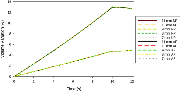
Figure 3.9 - NP and AF volume variation during extension. ... 44

Figure 3.10 - NP and AF volume variation during flexion. ... 44

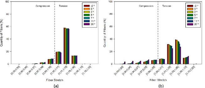
Figure 3.11 - AF fiber stretch during extension: (a) at 10s - end of pre-conditioning period; (b) 12s - end of loading period. ... 45

Figure 3.12 - AF fiber stretch during flexion: (a) at 10s - end of pre-conditioning period; (b) 12s - end of loading period. ... 45

Figure 3.13 - Angular range of extension-flexion movement. ... 46

Figure 3.14 - NP pressure variation during lateral flexion. ... 46

Figure 3.15 - AF pressure variation during lateral flexion. ... 47

Figure 3.16 - NP and AF volume variation during lateral flexion. ... 47

Figure 3.17 - AF fiber stretch during lateral flexion: (a) at 10s - end of pre-conditioning period; (b) at 12s - end of loading period. ... 48

Figure 3.18 - Angular range of bilateral flexion movement. ... 48

Figure 3.19 - NP pressure variation during axial rotation. ... 49

Figure 3.20 - AF pressure variation during axial rotation. ... 49

Figure 3.21 - NP and AF volume variation during axial rotation... 50

Figure 3.22 - AF fiber stretch during axial rotation: (a) at 10s - end of pre-conditioning period; (b) at 12s - end of loading period. ... 51

Figure 3.23 - Angular range of axial rotation movement. ... 51

Figure 3.24 - NP pressure variation during extension. ... 52

(20)

xviii

Figure 3.26 - AF pressure variation during extension. ... 53

Figure 3.27 - AF pressure variation during flexion. ... 54

Figure 3.28 - NP and AF volume variation during extension. ... 54

Figure 3.29 - NP and AF volume variation during flexion. ... 55

Figure 3.30 - AF fiber stretch during extension: (a) at 10s - end of pre-conditioning period; (b) at 12s - end of loading period. ... 55

Figure 3.31 - AF fiber stretch during flexion: (a) at 10s - end of pre-conditioning period; (b) at 12s - end of loading period. ... 56

Figure 3.32 - Angular range of extension-flexion movement. ... 56

Figure 3.33 - NP pressure variation during lateral flexion. ... 57

Figure 3.34 - AF pressure variation during lateral flexion. ... 57

Figure 3.35 - NP and AF volume variation during lateral flexion. ... 58

Figure 3.36 - AF fiber stretch during lateral flexion: (a) at 10s - end of pre-conditioning period; (b) at 12s - end of loading period. ... 58

Figure 3.37 - Angular range of bilateral flexion movement. ... 59

Figure 3.38 - NP pressure variation during axial rotation. ... 60

Figure 3.39 - AF pressure variation during axial rotation. ... 60

Figure 3.40 - NP and AF volume variation during axial rotation... 61

Figure 3.41 - AF fiber stretch during axial rotation: (a) at 10s - end of pre-conditioning period; (b) at 12s - end of loading period. ... 61

Figure 3.42 - Angular range of axial rotation movement. ... 62

Figure 4.1 - Schematic representation of a general MBS (Adapted from [89]). ... 63

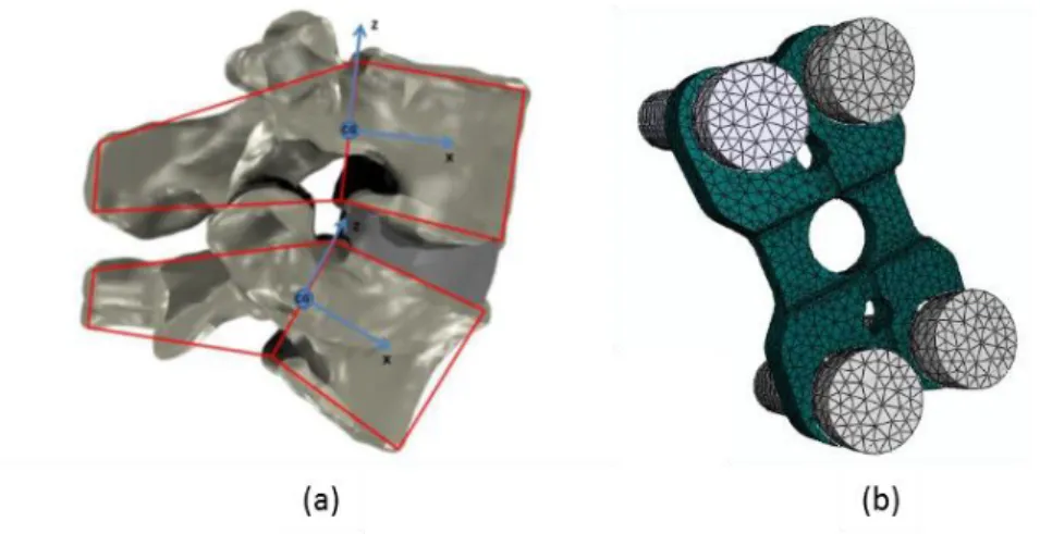
Figure 4.2 - Original model with the referential system highlighted. ... 65

Figure 4.3 - Schematic representation of the IVD modeling. ... 66

Figure 4.4 - Extension-flexion FEM results. ... 68

Figure 4.5 - Lateral flexion FEM results. ... 68

Figure 4.6 - Axial rotation FEM results. ... 69

Figure 4.7 - Segmentation and linearization of the L2-L3 Ex-Fx FEM result. ... 70

Figure 4.8 - Three-dimensional MBS model of the lumbar spine: (a) anterior view; (b) left lateral view; (c) posterior view. ... 71

(21)

xix

Figure 4.10 - Extension-flexion FEM and MBS simulation results of L1-L2... 73

Figure 4.14 - Extension-flexion FEM and MBS simulation results of L5-S1. ... 75

Figure 4.15 - Lateral flexion FEM and MBS simulation results of L1-L2. ... 75

Figure 4.19 - Lateral flexion FEM and MBS simulation results of L5-S1. ... 77

Figure 4.20 - Axial rotation FEM and MBS simulation results of all modeled IVDs. ... 78

Figure 4.21 - Comparison between experimental and simulation results of L1-L2 during Ex-Fx. . 79

Figure 4.25 - Comparison between experimental and simulation results of L5-S1 during Ex-Fx. 81 Figure 4.26 - Total range of motion during Ex-Fx of both experimental and simulation results. .. 82

Figure 4.27 - Comparison between experimental and simulation results of L1-L2 during LFx. ... 83

Figure 4.31 - Comparison between experimental and simulation results of L5-S1 during LFx. ... 85

Figure 4.32 - Total range of motion during LFx of both experimental and simulation results. ... 86

Figure 4.33 - Comparison between experimental and simulation results of L1-L2 during AR. .... 87

Figure 4.37 - Comparison between experimental and simulation results of L5-S1 during AR. .... 89

Figure 4.38 - Measured reaction forces (X-axis) when different loads are applied in X-axis. ... 90

Figure 4.39 - Measured reaction forces (Z-axis) when different loads are applied in X-axis. ... 91

(22)

xx

Figure 4.41 - Measured reaction forces (Z-axis) when different loads are applied in Y-axis. ... 92 Figure 4.42 - Measured reaction forces (X-axis) when different loads are applied in Z-axis. ... 93 Figure 4.43 - Measured reaction forces (Z-axis) when different loads are applied in Z-axis. ... 93

(23)

xxi List of Tables

Table 3.1 - Material properties of the model components. ... 36 Table 3.2 - Settings of the AF's fibers. ... 37 Table 3.3 - Inputted scale factors and resulting IVD heights. ... 39 Table 4.1 - World position, orientation and mass of the vertebrae (Adapted from [87]. ... 65 Table 4.2 - World position, orientation and thickness of all IVDs (Adapted from [87]. ... 66 Table 4.3 - Wedge angle of the different MBS lumbar levels and corresponding FEM model’s angle. ... 67 Table 4.4 - Segmentation parameters for L2-L3 Ex-Fx movement. ... 71

(24)

(25)

Co-Simulation of the Lumbar Intervertebral Discs through Finite Element Method and Multibody System Dynamics 1

1.1. Motivation and Scope

Chronic diseases have been frequently reported has the most common cause of mortality, with 63% of deaths worldwide. Since 2012, about half of all adults (117 million people) have one or more chronic health conditions. It is estimated that one of four adults has two or more chronic health conditions [1]. Seven of the top 10 causes of death in 2010 were chronic diseases, such as heart disease, stroke, cancer, chronic respiratory diseases or diabetes, among others. In the USA, the national health care system invests about 75% of their money in the treatment of chronic diseases. The principal consequences of these persistent conditions are lifelong disability, compromised quality of life, and burgeoning health care costs [2].

Among the wide range of chronic pathologies, chronic rheumatic conditions are a subgroup of diseases which include approximately 200 pathologies and syndromes that affect directly the musculoskeletal system, being progressively symptomatically and usually associated with acute pain. Musculoskeletal conditions are leading causes of morbidity and disability, giving rise to enormous healthcare costs and loss of work. Rheumatoid arthritis, osteoarthritis, osteoporosis, severe limb trauma and spinal disorders are the chronic rheumatic pathologies with more impact on the society [3].

Being the main cause for incapacity, spinal disorders include trauma, mechanical injury, spinal cord injury, inflammation, infection and tumor. About 80-85% of back pain episodes have unknown cause [4]. Spinal disorders are highly associated with rachialgia or back pain in the vertebral column. Low back pain (LBP) is the most common type of rachialgia, and it is considered a symptom rather than a disorder [5]. About 70-85% of the general population have LBP at some time in life. The annual prevalence of back pain ranges from 15% to 45% [6].

In the USA, low back pain is the most common cause of activity limitation in people younger than 45 years; the second most frequent reason for visits to the physician; the fifth-ranking cause

CHAPTER 1

(26)

2 Co-Simulation of the Lumbar Intervertebral Discs through Finite Element Method and Multibody System Dynamics

of admission to hospital; and the third most common cause of surgical procedures [7-9]. The data from western countries are similar. In the UK, LBP is the largest single cause of absence from work, and it is responsible for approximately 12.5% of all sick days [10]. Similarly, in Sweden, 11-19% of all 1987‘s annual sickness absence days were taken by people with a back pain diagnosis. About 13.5% of all reported sick days in Sweden happened due to back pain episodes. Overall, approximately 8% of the insured Swedish population were listed as sick with a diagnosis of back pain at some time during 1987 [11].

Lumbar disc disease has been identified as the most common cause of LBP [12]. This evidence became the motivation for this work, whose purpose is to study the biomechanical behavior of the lumbar IVDs in a healthy situation, which may posteriorly serve as a basis to study situations of degeneration and possible solutions for these disorders.

1.2. Literature Review

Throughout the years, the scientific community have been developing and optimizing mathematical models for biological simulation. Numerical modeling is an advantageous approach because it is non-invasive, low cost and it can reproduce the most complex aspects of the biological processes. In addition, numerical modeling can reproduce situations which would be hardly reproduced through other approaches. With the arise of high-speed computers, such models can become powerful tools to understand, prevent and help treat several health conditions or injuries [13,14].

Several models regarding specific spine components (articular facets, intervertebral discs (IVDs), ligaments, among others), motion segments (MSs), spinal regions or even the whole spine, are described in the literature. In such models, the most used computational methodologies are the finite element method (FEM) and multibody system (MBS) dynamics, being the finite element (FE) approach more frequently used in biomechanical studies of the human spine, due to a better and more complex representation of the spine components [15]. On the one hand, MBSs consist of rigid bodies linked through kinematic joints and elements applying forces. On the other hand, FE systems are able of producing highly detailed models by dividing the entities into smaller elements, connecting those by nodes, and producing the realistic material behavior by employing

(27)

governing equations into a FE algorithm. MBS models are less complex, requiring less computational power and simpler validation requirements, in comparison with FE models [16,17].

1.2.1. Finite Element Method approaches

The first spine models using FE approach were very simple in terms of geometry and material properties [18]. In 1974, Belytschko et al. developed a model with two vertebral bodies (VBs) and an IVD (with no internal morphology defined) with linear material properties [19]. In the coming years, researchers started to define the internal structures, and in 1977, Carter proposed a vertebral model with both trabecular and cortical bone [20]. Further advances concerned the implementation of the remaining spinal components, such as, articular facets (and the contact between them), ligaments and muscles [21,22].

With the advance on medical imaging techniques and reconstruction algorithms, the accuracy of the model’s geometry increased, being obtained from computed tomography (CT) or magnetic resonance imaging (MRI) [23]. With the arise of more accurate experimental data and constitutive equations, the materials properties became more complex, enhancing the understanding on the mechanical response of the different spine components [24].

Due to its complex biomechanical behavior, the IVD is the most critical component on FE modeling of the spine [25]. The evolution of FE modeling of the IVD concerned not only its material properties, but also its geometry ranging from two-dimensional to patient-specific three-dimensional models obtained by medical imaging reconstruction [26,27].

In early models, the IVD components consisted of only one phase with a simple linear elastic representation [28]. Such models presented inaccurate results, as the nonlinear behavior of the disc under loading was not considered [29].

In 1999, Kumaresan et al. provided a FE model with an improved representation of the annulus geometry and material properties, considering the existence of concentric laminae of collagen fibers [30]. Posteriorly, similar models were developed with collagen fibers modeled as tension-only elements [31] or rebar elements with a fixed inclination [32].

(28)

The following FE models started to incorporate radially dependent inclination and stiffness for the collagen fibers as described by Schmidt et al., and the material properties used for these elements were linear elastic or viscoelastic [33].

In several studies, the nucleus pulposus (NP) was modeled as an incompressible hydrostatic material [32,34]. Wang et al. presented, in 1997, a three-dimensional model of a lumbar IVD concerning both nucleus and annulus (with its collagen network) material properties [35]. The FE mesh of the model highlighting the different structures is presented in Figure 1.15.

Figure 1.1 - FE mesh of the L2-L3 MS model of Wang et al. highlighting its different structures (Adapter from [35]).

The work of Simon et al., in 1985, described the introduction of biphasic formulation in the mechanical properties of the IVD. This FE formulation considers two phases, one liquid and one solid [36]. This model was later improved with the incorporation of swelling pressure and osmotic pressure by Laible et al. and Simon et al. [37,38].

In 2004, Ferguson et al. proposed coupled poroelastic and mass transport FE models to predict the influence of load-induced fluid flow on mass transport within the disc. Their aim was the determination of the fluid flow patterns within the IVD resulting from the average diurnal spinal loading and the analysis of the relative contribution of diffusion and convection to solute transport in the IVD [39]. Figure 1.16 shows the FE mesh, emphasizing the different structures.

(29)

Figure 1.2 - FE model a lumbar IVD proposed by Ferguson et al. The different colors of the three-dimensional mesh represent the distinct components of the IVD (Adapted from [39])

Natarajan et al. developed, in 2007, a poroelastic FE model of the IVD (Figure 1.17) incorporating the swelling pressure and the effect of strain on the IVD permeability. The model was simulated in order to predict the failure initiation and progression in a lumbar disc due to repeated loading [40].

Figure 1.3 - FE model of a L4-L5 MS proposed by Natarajan et al. (Adapted from [40]).

In 2007, Schroeder et al. proposed an osmoporoviscoelasticity formulation to model the material properties of the IVD. Such formulation considers the IVD’s microstructure (composition) to model the material properties, including the contribution of the elastic nonfibrillar solid matrix, the viscoelastic collagen fibers and the osmotically pre-stressed permeable extrafibrillar fluid [41]. Figure 1.18 depicts the IVD’s FE mesh.

(30)

Figure 1.4 - FE mesh of one quarter of an IVD proposed by Schroeder et al. (Adapted from [41]).

The work of Strange et al., in 2010, described a three-dimensional FE model of the L4-L5 IVD (Figure 1.19), where the NP was modeled as a hyperelastic solid and the AF as a matrix of homogenous ground substance reinforced by rebar elements. The model was used to verify if an elastomeric implant for a nucleotomized IVD approximates the nucleus properties under compressive loading [42].

Figure 1.5 - Three-dimensional FE mesh of a lumbar IVD developed by Strange et al. (Adapted from [42]).

Huang et al. proposed, in 2014, a three-dimensional FEM model of a lumbar (L4-L5) MS (Figure 1.20) to simulate the biomechanical behavior of herniated discs. The model’s geometry was obtained from high-resolution computed tomography (CT). Both NP and AF were modeled as isotropic, incompressible and hyperelastic materials. Quadrilateral shell elements were used to model the CEPs. In addition, the vertebrae comprised both cortical and cancellous bone, and seven spinal ligaments were implemented with linear behavior. The model was simulated in several herniation stages, with NP removal and NP replacement. Results reveal the feasibility of this model for studies concerning the mechanical characterization of NP removal and the mechanical stability of NP removal [43].

(31)

Figure 1.6 - Huang's FE mesh of (a) the lumbar MS, (b) a healthy disc, (c) a mildly herniated disc, (d) a severely herniated disc, (e) a mildly herniated disc with NP removal, and (f) a severely herniated disc with NP removal. (Adapted from [43]).

In 2013, Castro developed a MS FE model that included an IVD with a novel osmo-hyper-poro-visco-elastic formulation reinforced by anisotropic AF fibers. The model was implemented within a custom FE solver under several loading profiles, being validated with both experimental and numerical data. The simulation’s main outcomes concerned displacement, pressure, volume variation and fiber stretch of the lumbar IVD. This model proved to be a reliable tool for understanding and reproducing the IVD’s biomechanics [44,45].

Figure 1.7 - Anterior-posterior cut of the FE mesh of a lumbar MS developed by Castro (Adapted from [44]).

The IVD FE models may be used to simulate normal and irregular situations (disc degeneration) experienced by the disc, being powerful tools to understand the mechanical behavior of this structure, and providing a significant contribute to help the prevention and treatment of disorders associated to the IVD.

(32)

1.2.2. Multibody System Dynamics approaches

The development of spine models, using both MBS and FEM formulations, has evolved greatly since 1957, when Latham described an analytical model of the spine, aiming to study pilot ejections [46]. The MBS first spine models were unsophisticated, consisting of a small number of rigid bodies linked by simple mechanical joints. Such models provided a first approach to the complex mechanical response to impact of the whole spine [47].

In 1981, Merril developed a model with ten rigid bodies, representing the head, cervical and thoracic vertebrae that were connected by massless springs and hysteretic elements. Seven pairs of muscles were also modeled as linear elements [48], being the number of muscles later increased to twenty eight [49].

Two years after, in 1983, Williams and Belytschko developed a three-dimensional human cervical spine model for impact simulation. Rigid bodies modelled the head and cervical vertebrae, which were interconnected by deformable elements representing the IVDs, facet joints, ligaments and muscles. The most relevant novelty presented in this model was the pentahedral continuum element which represented the facet joint, allowing both lateral and frontal plane motion [17].

Based on the work of Merrill et al. [48,49], Deng et al. defined a computational model for predicting sagittal-plane motion of the human head-neck during impact. The model was validated against frontal and lateral acceleration impacts results, from physical spine models and from volunteers. It was composed by human cervical and thoracical vertebrae, assumed as rigid bodies interconnected by intervertebral joints, an also fifteen pairs of muscles, represented as linear elements. Nonetheless, the individual contributions other structures involved in a intervertebral joint, such as ligaments, were not implemented [50].

In 1996, Broman at al. developed a numerical model of the lumbar spine (Figure 1.1), pelvis and buttocks to study the influence of vibrations from the seat to the third lumbar vertebra (L3), of individuals in sitting posture. The skeletal system was defined as rigid and soft tissues were modeled as linear components [51].

(33)

Figure 1.8 - Modeling components from the work of Broman et al. (Adapted from [51]).

The study of Stokes et al., in 1999, described the development of a rigid model (Figure 1.2) to study muscles and spinal forces. This model consisted of five lumbar vertebrae, twelve thoracic vertebrae, the sacum and sixty-six muscles. Two models with the same geometry and different properties were created: (i) the stiffness model, with the vertebrae modeled as beams with predetermined stiffness properties, and (ii) the static model, with the vertebrae were interconnected by ball-and-socket joints. Both models were subjected to flexion, extension, lateral bending and axial torque [52].

Figure 1.9 - Schematic representation of the models by Stokes et al.: (a) Stiffness model; (b) Static model (Adapted from [52]).

In 2000, De Jager improved the work of Deng et al. [50] with the implementation of active muscle behavior and by lumping the behavior of all soft tissues into the intervertebral joints. Their model was developed in three stages: (i) a global head-neck model was built with rigid head and vertebrae, linked through three-dimensional nonlinear viscoelastic elements that lumped the IVD’s

(34)

characteristics, ligaments and facet joints; (ii) detailed segments of the cervical spine were proposed, with three-dimensional elements for the IVD, nonlinear viscoelastic elements for the ligaments, and frictionless contacts in the facet joints; (iii) Hill-type muscles were included in the model [53]. Figure 1.3 depicts the schematic representation of De Jager’s global model with local coordinate system.

Figure 1.10 - Partial representation of De Jager's model (Adapted from [53]).

After several tests, calibration with data from human volunteers, De Jager concluded that the active muscle behavior was essential to describe the system’s response to impact and that his model was computationally efficient [53].

Waters et al. developed, in 2003, a MBS model for the assessment of low back disorders due to occupational exposure to jarring and jolting from operation of heavy mobile equipment. Firstly, the model comprised seventeen rigid bodies, which was later replaced by a simpler approach. The model consisted of four rigid bodies representing head/neck and upper, middle and lower torso, linked by spring-damper sets. It was used to simulate spinal motion [54]. A schematic representation of such model is presented in Figure 1.4.

(35)

Figure 1.11 - Human spine MBS model developed by Waters et al. (Adapted from [54]).

A study of Ishikawa et al. described, in 2005, a musculoskeletal dynamic spine model (Figure 1.5) that was able to perform functional electrical stimulation, spine motion simulation and stress distribution analysis. The skeletal geometry was built from computed tomography (CT) data from one healthy volunteer. Afterwards, muscles were added to the model using Nastran® software, and

IVDs and ligaments were modeled as spring-damper sets. Dynamic simulation was performed using Nastran® [55].

Figure 1.12 - Three-dimensional MBS model of the human spine developed by Ishikawa et al.: (a) General view; (b) Detailed representation of the IVDs and ligaments (Adapted from [55]).

In 2006, Esat developed a hybrid model of the whole spine with active-passive muscles and geometric nonlinearities. This model comprised a MBS used for dynamic analysis of impact situations, and a FE analysis to study the causes of spinal injuries. CT imaging data was used to build the model’s geometry. The vertebrae were modeled as rigid bodies, linked by linear

(36)

viscoelastic IVD elements, nonlinear viscoelastic ligaments and contractile muscle elements with both passive and active behavior. Contact forces were disregarded in this model [17]. Figure 1.6 depicts the lumbar region of Esat’s MBS model.

Figure 1.13 - Lumbar spine MBS model developed by Esat (Adapted from [17]).

Ferreira established, in 2008, a three-dimensional cervical MBS spine model with seven rigid bodies (head, seven cervical vertebrae and the first thoracic vertebra), linked by six bushing elements with six DOF each (playing the role of the IVD) and constrained by nonlinear viscoelastic elements simulating the spinal ligaments. Contacts between spinous processes and facet joints were implemented as sphere-plane nonlinear contact forces, following the Kelvin-Voigt formulation. The model aims to simulate the traumatic and degenerative disorders, such as rheumatoid arthritis [56]. In Figure 1.7 are presented the sagittal and frontal views of the model during an impact situation.

Figure 1.14 - Sequential representation of the lateral impact of Ferreira's model: (a) lateral view; (b) frontal view (Adapted from [56]).

(37)

The work developed by Juchem, in 2009, comprised a three-dimensional computational model of the lumbar spine (Figure 1.8) for mechanical stress determination. Five rigid bodies modeled the last four lumbar vertebrae and the sacrum. Geometry data was obtained through CT measurements. MBS formulation was applied and the IVDs were modeled as elastic elements. The effect of ligaments and facet joints were also implemented. The model was simulated with an applied load of 395 N at the top of the second lumbar vertebra mimicking the upper body’s weight. Thus, the reaction forces and torques of each IVD, and the reaction forces of ligaments were calculated [57].

Figure 1.15 - Three-dimensional model of the lumbar spine developed by Juchem (Adapted from [57]).

Monteiro, in 2009, proposed a hybrid model (Figure 1.9) of the cervical and lumbar spine model, using both FEM and MBS. His model aimed the analysis of the intersomatic, or vertebral fusion of one or more spine levels. MBS formulation was used to model vertebrae as rigid bodies, IVDs as linear viscoelastic bushing elements, ligaments as nonlinear elastic springs, and spinal contacts according to the nonlinear Kelvin-Voigt contact model. Muscles were disregarded from the model. FEM modeling was applied to the four IVDs with greater incidence of degeneration, and to the fixation plate (used for intersomatic fusion). A 1.5 Nm torque was applied to the first lumbar vertebra (L1) for 400 ms, while the sacrum (S1) was fixed. A 500 N load submitted to the upper surface of L1 was used to simulate the upper body weight. The model confirmed its capacity of predicting accurately axial rotation and extension movements [58].

(38)

Figure 1.16 – Lumbar hybrid model developed by Monteiro: (a) three-dimensional MS; (b) FE mesh of the fixation plate and screws (Adapted from [58]).

In 2010, Christophy developed an open-source musculoskeletal model of the human lumbar spine, focusing on the effect of muscles during spinal motion. The 6 DOF intervertebral joints and the muscles are governed by the Hill-type and Thelen’s muscle models. The model was simulated in flexion-extension movement focusing on the L5-S1 joint. Results revealed different behaviors of two groups of muscles: (i) the primary flexor muscles generated signigicant larger moments (approximately 60 Nm) than the (ii) stabilizer muscles (approximately 10 Nm). Despite the results, the lack of ligaments and contact between facet joints limits the accuracy of the model [59]. Figure 1.10 depicts two different configurations of the model (neutral and in 50º flexion) where muscles, rigid bodies and intervertebral joints are evidenced.

Figure 1.17 - Cristophy's three-dimensional musculoskeletal model with 238 muscles, 13 rigid bodies and 5 intervertebral joints: (a) neutral posture; (b) 50° flexion (Adapted from [59]).

(39)

On the study of Abouhossein et al., in 2010, a three-dimensional MBS lumbar spine model (Figure 1.11) was proposed. The model aimed the determination of load sharing between the passive elements of the lumbar spine. It consisted of six rigid bodies for the five lumbar vertebrae and the sacrum, six DOF nonlinear flexible for the IVDs, tension-only force elements for ligaments, and Kelvin-Voigt contact forces between facet joints. Muscles were not implemented in the model. To validate the model, in vitro data was used to compare the response of pure torque loading of kinematic and facet joint forces [60].

Figure 1.18 - Representation of the lumbosacral spine model developed by Abouhossein (Adapted from [60]).

Galibarov et al. described, in 2011, a computational model to investigate the muscular and external forces effects on the lumbar spine’s curvature. The model was implemented in Anybody Modeling System® software, where IVDs and ligaments were modeled as spherical joints and

nonlinear springs, respectively. Figure 1.12 represents the three-dimensional MBS model, highlighting both ligament and IVD elements [61].

(40)

Figure 1.19 - Lumbar spine MBS model of Galibarov et al. highlighting: (a) the lumbar ligaments (red segments); (b) the IVDs (red spherical joints) (Adapter from [61]).

In 2012, Han et al. developed a thoracolumbar spine model (Figure 1.13) for muscle force prediction. The bones of the model consisted of the skull, arms, legs, pelvis and spine. Cervical and thoracic spine were modeled as single elements. The lumbar region comprised the five rigid bodies linked by rigid spherical joints for the IVDs. Muscles were modeled as single force components. The model’s response was validated based on literature data [62].

Figure 1.20 - Lumbar MBS model developed by Han et al. with emphasis to (a) muscle segments, and (b) ligaments (Adapted from [62]).

(41)

More recently, Huynh et al. proposed a bio-fidelity discretized musculoskeletal MBS spine model (Figure 1.14) for assessing the biomechanical behavior between healthy spines and spinal arthroplasty or arthrodesis. This model was generated in LifeMOD® software, and comprised several

torsional spring forces representing the IVDs. Back ligaments and muscles were added from the software’s default library, and their mechanical properties were optimized using literature data. Simulations were performed for different postures and different loading conditions. The model was validated with both experimental data and in vivo measurements, proving to be a reliable tool to study spinal disorders [63].

Figure 1.21 - Musculoskeletal spine model developed by Huynh et al.: (a) frontal view; (b) lateral view (Adapted from [63]).

Since the first biomechanical spine studies, MBS models evolved significantly, not only in terms of number and type of elements modeled, but also in their complex geometry. This evolution has allowed a more accurate reproduction of the several anatomical elements (muscles, ligaments, facet joints, among others) involved in the biomechanical response of the human spine. The implementation of these different structures in the current models increases their complexity, but allows for a more realistic understanding of the spinal functioning by considering their physiological role in the biomechanics of the spine.

(42)

1.3. Objectives

The main goals for the present work are comprised in two phases: first, (i) a geometric sensibility study of the lumbar IVD through FE analysis, and second, (ii) the optimization and validation of a three-dimensional lumbar spine MBS model by implementing the previous FE results.

This research was performed within the co-operative European project “NP Mimetic – Biomimetic Nano Fibre-Based Nucleus Pulposus Regeneration for the treatment of Degenerative Disc Disease” (ref. NMP-2009-SMALL-3 CP-FP 246351).

1.4. Structure of the thesis

The present dissertation contains 5 chapters.

Chapter 1 presents the motivation of this work, a literature review on both FE and MBS modeling approaches of the human spine, and the main objectives of the present work.

Chapter 2 focuses on the spine characterization, giving an anatomophysiological description of the spinal components and the associated disorders.

Chapter 3 contains a brief description of the FE formulation and the IVD model. The IVD’s geometric sensibility analysis is also presented in this chapter.

Chapter 4 starts with the definition of MBS system, and then, a description of the lumbar model is presented. Posteriorly, the mechanical response of both FEM and MBS models are compared. Subsequently, the MBS model is validated using experimental data from the literature, and, finally the application of the model is presented.

Finally, the main conclusions and proposals for future work are enunciated in the Chapter 5. This dissertation ends with a full list of references consulted during the work development. As appendix, a table regarding the published range of motion of the lumbar vertebrae is presented.

(43)

CHAPTER 2 Spine characterization

2.1 Spinal Anatomy

The human spine or vertebral column is an anatomical structure located in torso’s posterior region, being extent from the base of the skull until the pelvis. It is responsible for the spinal cord and spinal nerves protection; body weight support; it has an important role in posture and locomotion; it allows the attachment of ribs, pelvis and back muscles; and it provides body flexibility [64]. Thirty-three vertebrae divided in five different regions constitute this structure:

• Cervical region, composed by seven cervical vertebrae (C1-C7) and its IVDsF. Their small VBs, partially bifid spinous processes and a transverse foramen in each transverse process, through which the vertebral arteries extend toward the head, characterize these vertebrae. Only cervical vertebrae have transverse foramina;

• Thoracic region, composed by twelve thoracic vertebrae (T1-T12) and its IVDs. Long and thin spinous processes inferiorly directed and relatively long processes are distinct characteristics of these vertebrae;

• Lumbar region, composed by five lumbar vertebrae (L1-L5) and its IVDs. Large and thick bodies, as well as heavy and rectangular transverse and spinous processes characterize lumbar vertebrae;

• Sacral region, composed by five sacral vertebrae fused into a single bone called sacrum; • Coccygeal region, composed by four fused vertebrae, the coccyx, also called tailbone. The coccygeal vertebrae are greatly reduced in size relative to the other vertebrae [64].

(44)

Figure 2.1 - Left lateral and posterior view of the human spine’s anatomy, with a lumbar MS highlighted (Adapted from [64]).

The five regions of the human spine have four major curvatures in the sagittal plane (Figure 2.1). These natural curvatures are anatomically named as lordosis (convex anteriorly) and kyphosis (concave anteriorly). Lordosis is present in the spine’s cervical and lumbar regions, while kyphosis is present in the thoracic, sacral and coccygeal region. These curvatures exist due to the non-homogeneous thickness of the IVDs. In the case of lordosis, the IVDs are thicker anteriorly than posteriorly. The opposite happens in the case of kyphosis, where the IVDs are thicker posteriorly than anteriorly [65]. In addition, these curvatures enhance the body weight support function of the spine [64]. IVDs (which connects two adjacent vertebrae allowing relative motion), as well as ligaments, muscles, articulations, neural and vascular networks are other anatomical elements that compose the human spine.

The smallest functional unit of the human spine is the motion segment (MS) (Figure 2.1). Two vertebrae connected by an IVD compose each one of these load-sharing units [66].

2.1.1. The vertebrae

The general structure of a vertebra consists of a VB, an arch and various processes (Figure 2.2). The vertebral arch projects posteriorly from the body and it is divided into left and right halves.

(45)

Each half has two parts, the pedicle, which is attached to the body, and the lamina, joining the lamina from the opposite half of the vertebral arch. The vertebral arch and the posterior part of the body surround a large opening called the vertebral foramen. The foramina of adjacent vertebrae combine to form the vertebral canal, where the spinal cord is contained. The vertebral arches and bodies protect the spinal cord [64].

Being the largest part of the vertebra, the body is a disc-shaped element with flat surfaces directed superiorly and inferiorly which is essential for loading support. It forms the anterior wall of the vertebral foramen. The IVDs are located between bodies [16].

Figure 2.2 - Superior, posterior and lateral view of a typical vertebra (Adapted from [16]).

The transverse processes extend laterally from each side the arch between the lamina and the pedicle. It serves as an attachment place for muscles and ligaments. The spinous processes are projected posteriorly at the point where two laminae join. It is also a site for muscle attachment, strengthening the vertebral column and enhancing movement ability. The spinous processes can be seen and felt as a series of lumps down the midline of the back. The laminae are the posterior parts of the arch and form the posterior wall of the vertebral foramen. The pedicles are the feet of the arch with one on each side of it forming the lateral walls of the vertebral foramen. The articular

(46)

processes are superior and inferior projections containing articular facets where vertebrae articulate with each other. The intervertebral foramina are lateral openings between two adjacent vertebrae through which spinal nerves exit the vertebral canal [64].

2.1.1.1. Lumbar vertebrae

As previously mentioned, vertebral characteristics are dependent of their spinal location. As described in Figure 2.3, lumbar vertebrae may be divided into three functional components: VB, pedicles and posterior elements. Each of these components has a unique role contributing to the integrated function of the whole vertebra [67].

Figure 2.3 – Lumbar vertebra divided by functional parts: (a) Vertebral body, (b) Pedicle, (c) Posterior elements (Adapted from [67]).

The main function of the VB is weight-bearing and its geometrical structure is designed (internally and externally) for that purpose. The lumbar region is subjected to approximately 80% of the compressive loads acting of the human spine. The VB’s superior and inferior flat surfaces are dedicated to supporting longitudinally applied loads. While the external design promote a better load support with large and thick bodies, the internal design enhances its response to dynamic loads. With a shell of cortical bone surrounding a cancellous core, the internal architecture is organized for the same load-bearing function. The cancellous core has a grid-like design of vertical and transverse trabeculae which not only enhances the weight bearing purpose of the VB, but also allows the existence of a vascular network [67].

The posterior elements of a vertebra are the laminae, the articular and the spinous processes. Collectively, they form a very irregular mass of bone, with various bars of bone projecting in different

(47)

directions. This happens because the various posterior elements are specially adapted to receive the different forces that act on the vertebra [67].

The pedicles are parts of the lumbar vertebrae, which normally are simply named and no specific function is assigned to them. However, they are the only connection between the VBs and the posterior elements. The bodies are designed for weight-bearing but they cannot resist sliding or twisting movements, while the posterior elements are adapted to be submitted to different forces. Thus, all forces sustained by any of the posterior elements are ultimately channeled towards the pedicles, which transmit the benefit of the forces to the VBs [67].

2.1.1.2. Sacrum

The sacrum consists of five vertebrae fused into a single bone. The transverse processes of the sacral vertebrae fuse to form the alae, which join the sacrum to the pelvic bones. The spinous processes of the first four sacral vertebrae are partially fused forming projections, called median sacral crest, along the dorsal surface of the sacrum. The spinous process of the fifth vertebra does not form, thereby leaving a sacral hiatus at the inferior end of the sacrum, which is often the site of anesthetic injections. The intervertebral foramina are divided into dorsal and ventral foramina, called the sacral foramina, which are lateral to the midline. The anterior edge of the first vertebra’s body bulges to form the sacral promontory, a landmark that separates the abdominal cavity from the pelvic cavity [64].

2.1.1.3. Coccyx

The coccyx or tailbone, is the most inferior portion of the vertebral column and usually consists of three to five fused vertebrae that form a triangle, with the apex directed inferiorly. The coccygeal vertebrae are smaller when compared to the other vertebrae and they have neither vertebral foramina nor well-developed processes [64].

2.1.2. Facet joints

The facet joints are formed by the articulation of a vertebra’s superior articular process and the inferior articular process of the vertebra directly above it. It is a synovial joint covered by hyaline cartilage. A synovial membrane bridges the margins of the cartilage of the two facets in each joint.

(48)

The friction between surfaces and the surface wear are decreased by hyaline cartilage and the lubrication of the synovial fluid, respectively. The ligamentum flavum and the posterior longitudinal ligament reinforce the joint capsule which surrounds the synovial membrane.

The lumbar spine articular facets have an ovoid shape, becoming oval from the first to the fifth lumbar vertebra. This joint is oriented perpendicularly to the transverse plane. Shape and orientation variations of the lumbar facet joints limit the movement of this region, specifically in the axial plane [67].

2.1.3. Intervertebral disc

The IVD is an anatomical element that connects two adjacent VBs. It consists of a highly inhomogeneous porous structure with solid and fluid materials [68]. Its complex structure is constituted by a central gel-like core, the nucleus pulposus (NP), which is laterally surrounded by a fiber-layered structure, the annulus fibrosus (AF). Cartilaginous endplates (CEPs) and vertebral endplates (VEPs) vertically limit the IVD. Figure 2.4 depicts the IVD’s anatomical organization.

Figure 2.4 - IVD’s anatomy: (a) a MS’s structural organization; (b) IVD’s detailed structures and dimensions (Adapted from [68]).

Lumbar IVDs are the thickest of all vertebral column, varying from 7 to 10 mm in height and from 35 to 55 mm in diameter (axial plane). Contrarily to other anatomical structures, the IVDs do not have blood supply, depending on mechanical means of water absorption for the nutrition process [69].

(49)

Beside its function of linking the adjacent vertebrae, the IVD provides flexibility, elasticity and compressibility to the spine, and it allows load transmission [69].

2.1.3.1. Nucleus Pulposus

The NP is the inner part of the IVD that consists of a gelatinous core made of collagen fibers (randomly arranged) and elastin fibers (radially arranged) embedded in a highly hydrated aggrecan-containing gel. Two major regions characterize the NP: a solidified porous center and a peripheral gel-like region. The mainly isotropic, almost incompressible and osmo-poro-visco-hyperelastic properties, as well as the biochemical composition and the spatial confinement between the AF and the CEP are the reasons for the particular mechanical behavior of the NP. Being neither exclusively a solid nor a fluid, the NP is considered a biphasic tissue [44,69].

2.1.3.2. Annulus Fibrosus

The AF is the peripheral part of the IVD, forming a ring around the NP, and consisting on a series of 15 to 20 concentric lamellae of collagen fibers arranged in a highly ordered pattern. Trace amounts of elastin fibers and proteoglycans can also be found in its biochemical composition.

In this structure, two sets of fibers cross obliquely to each other at about ±30 degrees in relation to the disc. The annulus peripheral layers are denser, more resistant to tensile forces and reinforced by the posterior and anterior longitudinal ligaments. The annular cells are fibroblast-like, elongated and generally aligned with the oriented collagen fiber arrays in the extracellular matrix. As one moves from the outer region into the NP, the cells become more oval, the collagen fibers lose density and organization, and the proteoglycan concentration increases. Functionally, the AF is capable of intradiscal pressure containment and intervertebral motion guidance [44,69].

2.1.3.3. Cartilaginous Endplate

The CEP is a thin horizontal layer (usually less than 1 mm thick) of hyaline cartilage. demThe collagen fibers within the CEP are oriented horizontal and parallel to the VBs. The CEP behaves as a mechanical barrier between the pressurized NP and the vertebral bone, as well as a pathway for nutrient transport into the disc from adjacent blood vessels. CEPs are distinct from the adjacent VEPs, which are composed of cortical bone [67,70].

(50)

Figure 2.5 - Components of the IVD (Adapted from [71]).

2.1.4. Ligaments

Ligaments are anatomical elements with a complex architectural hierarchy that link two or more bones. Structurally, they are composed by bands of connective tissue with an high water content (55-65%). The remaining dry matter (35-45% of the total weight) is divided in 70-80% type I collagen, 10-15% of elastin and 1-3% of proteoglycans [72]. The hierarchical organization of the ligament is depicted in Figure 2.6.

Figure 2.6 - Hierarchical organization of the ligament, components and respective dimensions (Adapted from [72]).

The major function of ligaments is the connection between bones, contributing to structural stability’s maintenance. In addition, they enable protection of the neural structures, physiologic

(51)

motion range and spine protection against excessive movements. Mainly, the ligament nomenclature depends on its location [73].

At the lumbar level, each MS has seven ligaments: the anterior longitudinal ligament (ALL), the posterior longitudinal ligament (PLL), the ligamentum flavum (LF), the interspinous ligament (ISL), the supraspinous ligament (SSL), the intertransverse ligaments (TTL) and the capsular ligaments (CL) [67]. All these structures can be observed in Figure 2.7.

Figure 2.7 - Ligaments of a MS (Adapted from [56]).

2.1.4.1. Anterior Longitudinal Ligament

The anterior longitudinal ligament (ALL) is described as a long band which covers the anterior surfaces of the VBs and IVDs. Although well developed in the lumbar region, this ligament is extended from the cervical region to the sacrum, covering the anterior surface of the whole human spine. Structurally, this ligament consists of several sets of collagen fibers. Some short fibers extend through each interbody joint, covering the IVDs and attaching to the margins of the VBs [67].

2.1.4.2. Posterior Longitudinal Ligament

Similarly to the ALL, the posterior longitudinal ligament (PLL) is represented throughout the vertebral column. In the lumbar region, it forms a narrow band over the back of the VBs but expands laterally over the back of the IVDs to give it a saw-toothed appearance. Its fibers mesh with the AF to attach to the posterior margins of the VBs [67].

(52)

2.1.4.3. Ligamentum Flavum

The ligamentum flavum (LF) is a short but thick ligament that joins the laminae of consecutive vertebrae. At each intersegmental level, the LF is a paired structure, being represented symmetrically on both left and right sides. On each side, the upper attachment of the ligament is to the lower half of the anterior surface of the lamina and the inferior surface of the pedicle. Histologically, the ligamentum flavum consists of 80% elastin and 20% collagen [67].

2.1.4.4. Interspinous Ligament

The interspinous ligaments (ISLs) connect adjacent spinous processes. The collagen fibers of these ligaments are arranged in a particular manner, with three parts being identified: ventral, middle and posterior part. These ligaments consist essentially of collagen fibers, but elastin fibers appear with the increasing density of the ventral part towards its junction with the ligamentum flavum [67].

2.1.4.5. Supraspinous Ligament

The supraspinous ligament (SSL) is located in the midline. It runs posteriorly to the posterior edges of the spinous processes, to which it is attached, and bridges the interspinous spaces. The SSL collagen fibers become denser from the superficial to the deepest layers [67].

2.1.4.6. Intertransverse Ligament

The intertransverse ligaments (TTLs) have a complex structure that can be interpreted in many ways. They consist on sheets of connective tissue extending from the upper border of one transverse process to the lower border of the transverse process above. Unlike other ligaments, they lack a distinct border medially or laterally, and their collagen fibers are not as densely packed, nor as regularly oriented as the fibers of other ligaments [67].

2.1.4.7. Capsular Ligament

In general, a capsular ligament (CL) is a part of the articular capsule that surrounds a synovial joint. In the vertebral column, the capsular ligaments are attached to the articular margins of the