Lat. Am. j. solids struct. vol.14 número9

Abstract

In this research, two stress-based finite element methods includ-ing the curvature-based finite element method (CFE) and the curvature-derivative-based finite element method (CDFE) are developed for dynamics analysis of Euler-Bernoulli beams with different boundary conditions. In CFE, the curvature distribution of the Euler-Bernoulli beams is approximated by its nodal curva-tures then the displacement distribution is obtained by its inte-gration. In CDFE, the displacement distribution is approximated in terms of nodal curvature derivatives by integration of the cur-vature derivative distribution. In the introduced methods, com-pared with displacement-based finite element method (DFE), not only the required number of degrees of freedom is reduced, but also the continuity of stress at nodal points is satisfied. In this paper, the natural frequencies of beams with different type of boundary conditions are obtained using both CFE and CDFE methods. Furthermore, some numerical examples for the static and dynamic response of some beams are solved and compared with those obtained by DFE method.

Keywords

Euler-Bernoulli beams, Stress-based finite element, Natural fre-quency, Dynamic analysis.

Stress-Based Finite Element Methods for Dynamics Analysis

of Euler-Bernoulli Beams with Various Boundary Conditions

1 INTRODUCTION

Displacement-based finite element (DFE) method has extensively been used in computational solid mechanics. In this method, the displacement and slope are used as the nodal values in the modelling of beams. The main disadvantage of DFE is the discontinuity in the stress distribution. Further-more, stress boundary conditions are not exactly satisfied which causes the inaccuracy of the ap-proximated solution. To eliminate the mentioned problem, stress-based finite element (SFE) has been introduced (De Veubeke, 1965; De Veubeke, 1967). In this method, stress distribution is ap-proximated by assumed stress function and the transverse deflections and slopes are obtained by

Majid Gholampour a

Bahman Nouri Rahmat Abadi a,* Mehrdad Farid a

William L. Cleghorn b

a_{School of Mechanical Engineering,}

Shiraz University, Shiraz, Iran.

b _{Department of mechanical and}

indus-trial Engineering, University of Toronto, Toronto, Ontario, Canada.

*Corresponding author: E-mail: bahmannouri@shirazu.ac.ir

http://dx.doi.org/10.1590/1679-78253927

integration. Consequently, the considered method provides the continuities of not only transverse deflection but also stress at nodes. This technique was used for analyzing different problems, such as Kirchhoff plates (Morley, 1968; Punch and Atluri, 1986), plane elastic problems (Watwood and Hartz, 1968; Wieckowski et al., 1999) and elasto-plastic analysis (Wieckowski, 1995; Kuo et al., 2006).

Kuo et al. (2006) introduced CFE method for Euler- Bernoulli beam. In their work (Kuo et al., 2006), a cantilever beam and a slewing beam were studied. After that, they used CFE (Kuo and Cleghorn, 2011) and SFE method (Kuo and Cleghorn, 2007) to study a four-bar mechanism and a flexible slider crank mechanism with small strain but large rigid body motion, respectively.

Later, Farid and Cleghorn (2012) utilized CFE method for the first time to model the dynamics of a single-flexible-link spatial manipulator. They also obtained the dynamic equations of planar multi flexible-link manipulators and verified the results with the displacement finite element method (Farid and Cleghorn, 2014). Furthermore, an improved curvature-based finite element method was developed in (Chen et al., 2015) for the dynamic modelling of a high-speed planar parallel manipu-lator with flexible links. Also, the method was used for solving a sliding beam problem (Kuo, 2015). The varying-length beam element was established for solving the considered problem.

To the best of our knowledge, the CFE method has been used for the analysis of the problems in which the beams are considered to be clamped-free. The main scope of the present research is to extend the CFE and to introduce CDFE method for vibration analysis of Euler-Bernoulli beams with different boundary conditions.

The paper is organized as follows: Section 2 introduces both stress-based finite element methods. In section 3, the shape functions of both CFE and CDFE methods are obtained for different bound-ary conditions in order to approximate the deflection in each element. In section 4, using La-grange’s equation, equations of motion are obtained and the natural frequencies of beams are ob-tained. Finally, in section 5, numerical examples related to the static and dynamic responses of some beams are investigated.

2 STRESS-BASED FINITE ELEMENT METHODS

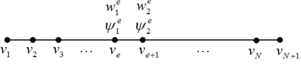
In Figure 1, the Euler-Bernoulli beam divided into Nelement is depicted. The transverse deflection,

slope and the nodal variable at the left end of the eth element are designated with w1e,1eandv1e,

while those at the right end are shown with, w2e,2e andv1e,respectively. Also, the ith global nodal

variable, vi in each of CFE and CDFE methods are considered miandni, respectively.

In sequence, the shape functions in each of the curvature and the curvature derivative-based fi-nite element methods are obtained.

2.1 Curvature-Based Finite Element Method (CFE)

The curvature distribution in the eth element, e

 

m  , can be linearly approximated as

 

 1( ) 1  2( ) 2

e e e

m  S  m S  m ₍₁₎

where, S1( ) _and S2( ) are considered as

1( ) 1  , 2( )

S   S   (2)

in which

1 ( ) /(  )  x xe xe xe

 (3)

The slope in the e_{th element,} e_{can be obtained by integrating Eq. (1).}

 

2 2

e e e

1 2 1

2 2

  

 _  _   _

 

 

e e

h  m  m c

   (4)

where, c1e is a constant. Considering the slope of the first node as0, the constant can be written as

1 0

1 1



c h



(5)

Using the continuity of slope between the first and the second element, the constant, c12 is

de-rived as

2

1 2 1 2 1 1 2 2 0

2 2

1 1 1

2 2

 

 _   _

 

c h h m h h m h

h  (6)

In general, the constant c1e for the eth element can be obtained in a similar way as

e

1 2 1 1 1 2 2 2 3 3

2 1 1 1 2 0

1 1_{[ (}1 1 _{) (}1 1 ₎

2 2 2 2 2

1 1 1

( )

2  2   2 

    

    _

e e e e e

e

e e e e e e e e

c h h m h h h h m h h h h m

h

h h h h m h h m h

(7)

Integrating Eq. (4), the transverse deflection in the e_{th element can be obtained by the} follow-ing equation.

 

2 3 3

e 2 e e e

1 2 1 2

2 6 6

  

 _  _    _

 

 

e e

In Eq. (8), c2e is a constant parameter determined by boundary conditions. Considering the

continuity of deflection at the internal nodes, the constant is obtained as

e 2 2 2 2 2 2 2

2 2 1 1 1 2 2 2 3 3 2 1 1

2 2 1 2 2 2 1 1

1 1 1 2 1 1 1 2

1 1 _{[ (}1 1 _{) (}1 1 _{) (}1 1 ₎

2 6 3 6 3 6 3

1 _]

6

  



 

      

    

e e e

e

e

e e e

c h m h h m h h m h h m

h

h m h c h c h c c

(9)

Using Eqs. (7-9), the deflection of the e_{th element is approximated as}

 

1

 

e e e e

1 0 2 0 1









N i i 

i

w  H  m N N w ₍₁₀₎

In the above relation, Hie

 

 , 1 e

N and N2e are the shape functions of the eth element obtained

as

For e ₌₁

2 3 2

11  1  ₂  ₆ 

 

H h   _(11-a)

For e = 3, 4, … ,N

2 1

e 1 1 1

1

2

3 2 2





 



e  e k k

h h

h h

H h  (11-b)

For e = 1, 2, … ,N

2 e e 1  ₆e

h

H  (11-c)

For e = 2, 3, …, N

2 2 3

2

1 1 _{( )}

6 2 2 6

   

e e e e

e e

h h h

H  h   (11-d)

For e = 3, 4, …. , N

2 2

e e 2 2 1 1 2 1

1 ₆ ₂  ₂  ₂ 

       

 

e e e e e

e e

h h h h h h

H h  _(11-e)

For e = 4, 5, …. , N

2 2

e e 3 3 2 2 3 2 3 2

2 1

6 2  3  2   2 

           

   

e e e e e e e

e e e

h h h h h h h h

H h h  _(11-f)

For i e 2,...,N 1

0



e i

where, N is the total number of elements. Also, N1e and N2e are derived as





1e  e  1 2 e1

N h h h h (12-a)

2e 1

N (12-b)

2.2 Curvature Derivative-Based Finite Element Method (CDFE)

The curvature derivative distribution in the e_{th element, n}e

 



_{, can be linearly approximated as}

 

 1( ) 1 2( ) 2

e e e

v  S  n S  n ₍₁₃₎

where, S1( ) and S2( ) are defined in Eq. (2). The curvature distribution in the beam can be

ob-tained by integrating Eq. (13).

 

2 2

e e e

1 2 1

2 2     _  _   _     e e

h n n c

m     ₍₁₄₎

The slope and transverse deflection of the eth element can be obtained by integrating Eq. (14) as

 

2 3 3

e 2 e

1 2e 1 2

2 6 6

    _  _    _     e e e

h   n  n c c

   (15)

 

3 3 4 4 e 2

1

2 2 3

e 1 ₂₄

6 24 2

  

 _  _     _

 

 

e e e

e

e

w  h   n  n c  c c ₍₁₆₎

in which, c1e, c2e and c3e are the constant parameters obtained by the continuity of curvature, slope

and deflection between elements. The constantsc1eand c2e are similar to the CFE method and the

constant c₃eis derived given as









2 1 1

2

1 1 1

3e 1 1 22 2 1 2

2

1 2 3

2 2 3 1 5 1 2

2 1 2

6

2

1 2

1 3 1 1

( ) ( 4) ( )

3 4 2 6 6 4 2 2

1 3_{( 4)} 1 1

1 _{[ (}1 1 ₎

3

1 1 ₍

( ) 3 1 1 ( 3 )

6 6 4 2 2

1 3

6 6 4

                _   _ _   _{ }             _   _ _   _{ }                  







e e k k k k e e k k

c h h h h n h h e e k h h h n

e e

h

h h n

h h

k h h h





1

2 1 2

5

3 2 3

1 2

1

1

)

1 1

( 4) ( )

2 2

( ) ]

8 6 4 24

          _ _  _{ }  _               



e k k

e e e e

e

e

e

e e k h h h

h h n h h n n (17)

The deflection of the eth element in the CDFE method can be written as

 

1

 

1 2 0 3 0

1 0

 

  





N

e e e

i

e e

i i

in which, the shape functions e

 

i

H  are obtained as

For e ₌₁

3 4 1 3

1  1  ₆ ₂₄

 

H h   _(19-a)

For e = 3, 4, …, N

2 1

e 13 1 1 2 1

1 1

2

+ + ) ( 1) 4 3

8 4 ( 2





 



e k  

k

h h h h e

H   h  h _(19-b)

For e = 1, 2, … , N

3

e 4

e 1 ₂₄e h

H  (19-c)

For e = 2, 3, …,N

2

1 1 1

3 2 3 4

3_{( )}

24 6 4 6 24

    

e e e e

e e

h h h

H   h   (19-d)

For e = 3, 4, …. ,N

3 3 2 2 2

e e 2 e 1 e 2 1 e 2 e 1 2 1 1 2 2 2

1 ₂₄ ₈ ₆ ₄ ₆ ₃ ₆  ₄ ₁₂

     e    e e  e  e

e

h h h h h h h h h h

H      (19-e)

For e = 4, 5, …. , N

2 2

e e 33 e 2 e 3 3 2 3 1 3 2 2 3

2

2

3 2 3 2

3 2

3 4 6 3 2

2

24 8 3 6

4

          



   

        

 

   

 _{ }  _{ }

   

e e e e e e e e

e

e e e e

e

h h h h h h h h h h h

H

h h h h

h

  

  (19-f)

For i e 2,...,N 1

0 

e i

H (19-g)

Furthermore, 1

e

N , 2

e

N and 3

e

N _{are derived as}





2

2

1e 1₂ e  1 2 e1 ( 1)₂

e

N h h h h  (20-a)



1



2e e   2 e1

N h



h h h _(20-b)

3e 1

N (20-c)

3 BEAMS WITH DIFFERENT BOUNDARY CONDITIONS

In this section, the unknown constants in Eqs, (10) and (18) are obtained by considering the boundary conditions. In CFE method, two of the boundary conditions are used to determine the constants 0 and w0, the other boundary conditions are incorporated as constraints. In CDFE

method, the constant m0, 0 and w0 are obtained by using three boundary conditions and the

other one is imposed as constraint.

Therefore, the deflection of the elements in the CFE and CDFE methods can be written in terms of nodal variables as

 

1

 

1









N

e e

i i

i

w  H  v ₍₂₁₎

In what follows, the shape functions, e

 

i

H  in the CFE and CDFE methods are obtained for

different boundary conditions such as clamped-free, pinned-pinned, pinned-guided, clamped-pined, clamped-guided and clamped-clamped.

3.1 Clamped Free (CFE)

For the clamped free beam, the deflection and slope of the first node are zero and the boundary conditions are written as









1 _{ 0} 1 _{ 0 0}

w    ₍₂₂₎

Thus, 0 and w0 are zero and the shape function Hie are obtained the same as e i

H .

3.2 Clamped Free (CDFE)

For the clamped free beam, the constants w0, 0 and m0 in Eq. (18), are obtained using the

follow-ing conditions













1 _{ 0} 1 _{ 0} N _{ 1 0}

w    m  (23)

Constants 0 and w0 are zero and the following relation for m0 is derived

















0 1 1 2 2 1 1

1

1 _{[ 1 1 1 ]}

1    

  _{ } N   N   N 

N N N

m H n H n H n

N     (24)

Therefore, the shape functions can be presented in the form of Eq. (21), where e i

H is obtained as









1

1 1 1,2,

1

1 _{   ..., 1}  _{  }

e e e e

i

i i N

H H N H i N

3.3 Pinned-Pinned (CFE)

In this case, the boundary conditions are given as









1 _{ 0} N _{ 1 0}

w  w  (26)

Considering the first boundary condition, constant w0 is zero. Incorporating, the second

bound-ary condition, constant 0 is obtained as



 











0 1 1 2 2 1 1

1

1 _{[ 1 1 1 ]}

1  

  _ e   e   e 

N N

e H m H m H m

N

 _    (27)

By substituting Eq. (27), to Eq. (10), the deflection of the nodes is obtained in which the shape function, e

i

H is obtained as









1 1

1 _{1 1,2,..., 1} 1

 e _ N N   

i i

e

i e

H H N H i N

N   (28)

3.4 Pinned-Pinned (CDFE)

Since the deflection and the curvature at the left side of the beam are zero, constants w₀ and m₀ are zero. Constant 0 can be obtained by considering zero deflection at the left side of the beam as

















0 1 1 2 2 1 1

1

1 _{[ 1 1 1 ]}

1  

  _     N 

N

N

N N

N H n H n H n

N

   

 (29)

In this case, the deflection of the beam can be written in the form of Eq. (21), where e i H is ob-tained similar to the pined-pined beam in CFE method given in Eq. (28).

3.5 Pinned-Guided (CFE)

For the pinned-guided case, the boundary condition are written as









1 _{ 0 }N _{1 0}

w  w  (30)

Considering the boundary conditions, the unknown parameter, w0is zero and the parameter 0

is derived as

















0 1 1 2 2 1 1

1

1 _{1 1 1}

1    

  _{  } e   e    e  _

N N

e H m H m H m

N

 _    (31)

Using Eqs. (31), and (10), the nodes’ displacement of the pinned-guided beam is derived where, e

i

H is obtained as









1

1

1 _{1 1,2,..., 1} 1   

  _ 



e

i e

e N N

i i

H H N H i N

3.6 Pinned-Guided (CDFE)

Considering the following conditions













1 _{ 0} 1 _{ 1 }N _{ 1 0}

w  m  w  (33)

Constants w0 and 0 are zero and m0is derived obtained as

















0 1 1 2 2 1 1

1

1 _{1 1 1}

1    

  _      

    

N H N n H N n  HNN nN m

N     (34)

In this case, the shape functions can be derived as given in Eq. (32).

3.7 Clamped-Pinned (CFE)

Considering zero deflection and slope for the first node, the shape functions are obtained similar to the clamped free beam in the CFE method. The zero displacement at the right end is considered as a constraint where can be obtained by multiplying the matrix Γ by the vector of curvature. The matrix Γ is given as









1 1 1 1

 

_   _

Γ N  N

N

H  H  ₍₃₅₎

3.8 Clamped-Pinned (CDFE)

Using the following conditions













1 _{ 0 }N _{1 } N _{ 1 0}

w  w  w  (36)

Constants w0 and 0 are zeros and m0 is found as

 

 

 

 

0 1 1 2 2 1 1

1

1

₁

₁

₁

1



 



 

_







 



_





N N

N N

N

N

H

n

H

H

n

N

m





n





(37)

By substituting Eq. (37), to Eq. (18), the deflection of the nodes is obtained in the form of Eq. (28).

3.9 Clamped-Guided (CFE)

In this case, the shape functions are similar to the clamped-free beam in CFE method. Also, the zeros slope at the right end of the beam is considered as a constraint. In this case, the matrix Γ is defined as









1 1 1 1

 

_   _

Γ N  N

N

H  H  ₍₃₈₎

3.10 Clamped-Guided (CDFE)





1









1 _{ 0  1  }N _{ 1 0}

w  w  w  (39)

Constants w0 and 0 are zero and m0 is derived as

 

 

 

 

0 1 1 2 2 1 1

1

1

₁

₁

₁

1



 



 

_







 

















N N N

N N

N

H

n

H

n

H

n

m

N









(40)

The shape functions are similar to Eq. (32).

3.11 Clamped-Clamped (CFE)

For beams with this boundary condition, the shape functions are similar to those of the clamped-free beam in CFE method. Furthermore, the constraints are zero displacement and zero slope at the right end of the beam which can be obtained by multiplication the matrix Γ to the curvature vec-tor. In this case, matrix Γ can be presented as

























N N N

1 2 N 1

1 2 1

1

1

1

1

1

_

1











 

_

_

_













Γ





N N N

N

H

H

H

H

H

H













(41)

3.12 Clamped-Clamped (CDFE)

In this case, the conditions are





1













1 _{ 0   1} N _{0  }N _{1 0}

w  w  w  w  (42)

Constants w0 and 0 are zero and m0 is obtained as

 

 

 

 

0 1 1 2 2 1 1

1

1

₁

₁

₁

1



 



 

_

_

N





N



 





_

N N

N

N

H

n

H

H

n

N

m





n





(43)

The zero slope at the right side of the beam is considered as a constraint which, can be obtained by multiplying matrix Γ by curvature derivative vector













1 1 2 1 1 1

 

_    _

Γ N N  N

N

H  H  H  ₍₄₄₎

The shape functions can be seen in Eq. (28).

4 FREQUENCY EQUATION

In this section, using Lagrange’s equation and the assumed deflection of the eth element in terms of nodal curvatures and curvature derivatives in CFE and CDFE methods, respectively, the mass ma-trix and stiffness mama-trix can be obtained.

4.1 Mass Matrix

0 2 1

1 ₍ 2  )





e

e w

d t

T A  ₍₄₅₎

where, the density and the cross area of the beam are designated with constants



and A, respec-tively. Using Eqs. (21) and (45), the kinetic energy can be rewritten as

1 1 1 e

1 1 0

1 2

 

 





N N e e 

i j i j i j

T A H H v v d ₍₄₆₎

Thus, the components of the e_{th element mass matrix are}

1 e

0





e e

ij i j

m A H H d ₍₄₇₎

Also, the kinetic energy of a beam carrying a concentrated mass, m0 attached at the eth global

node is given as

1 1 0

1 1

( 1) ( 1) 1

2

 

 





N N e  e   

i j i

i j

j

T m H  H  v v ₍₄₈₎

Therefore, the corresponding components of the eth element mass matrix can be obtained as

e

0 ( 1) ( 1)

 e  e 

ij i j

m m H  H  ₍₄₉₎

4.2 Stiffness Matrix

The potential energy of the eth element of the Euler beam can be written as

2

1 2 e

e e

2 0

1 2

   _{ }  



w

U EI d

 (50)

in which, e

EI is the flexural stiffness of the eth element. Considering the transverse deflection of the eth element, the component of the eth element stiffness matrix can be obtained as

1

e e

0

  

_

e e

ij i j

k EI H H d ₍₅₁₎

where, e i

H is the second derivative of e i

H .

If linear and torsional springs with stiffness kl and kt are attached to the eth global node, the corresponding component of the stiffness matrix can be obtained as

e _ e_{( 1) (}e _{1) }e_{( 1) }e_{( 1)}

ij l i j t i j

k k H  H  k H  H  ₍₅₂₎

Remark: The size of the total mass and stiffness matrices of the spring-mass-beam system is

4.3 Load Vector

The virtual work of a discrete load, Fk acting at the eth node can be written as





. 1

 e 

k k

W F w

   (53)

While the virtual displacement of each node is as

 

1

 

1









N

e e

i i

i

w H v

    (54)

Using Eqs. (53) and (54), the generalized force can be written as

 

fk Fk (55)

where, the vector  is defined as













1 1 2 1 1 1      _        _        e e e N H H H    (56)

The generalized force vector associated to a concentrated moment, Mk at the eth node can be written as

 

fk Mk (57)

where, the vector  for the moment is obtained as













1 2 1 1 1 1       _{ }        _{ }        e e e N H H H    (58)

Furthermore, it can be shown that the generalized force vector due to a continuous force, f ξ

 

and a continuous moment, M

 

ξ in the eth element can be obtained from Eqs. (59) and (60), re-spectively.

  



  



 





1 1 0 1 2 0 1 1 0

f ξ 1

f ξ 1

f ξ _ 1

  



  



 





1

1 0

1

0 2

1

1 0

ξ 1

ξ 1

ξ _ 1

 _{ } 

 

 _{ } 

 

  

 

 _{ } 

 

 







f



e

e

M

e N

M H d

M H d

M H d

 

 

 

(60)

The i_{th column of the assembled load vectors is obtained by summation the ith column of the} elements.

4.4 Natural Frequency

Using the obtained assembled mass and stiffness matrices, the dynamic equation of a beam without constraint can be written as

 f v

M Kv (61)

The natural frequencies of these beams can be obtained from the following eigenvalue relation

2 ₀

 

K  M (62)

For the beams with constraints, by incorporating the constraints, the resulting differential alge-braic equations can be written as

0

0 0 0 0

  

   _    _

 

                

M v K Γ v f

p Γ p

 T

(63)

in which, the vector of reaction force is presented by p.

The natural frequencies for these beams can be obtained by solving the following equation

2 0 ₀

0 0 0

  _   _   _ _

 

M

K Γ

Γ

T

 (64)

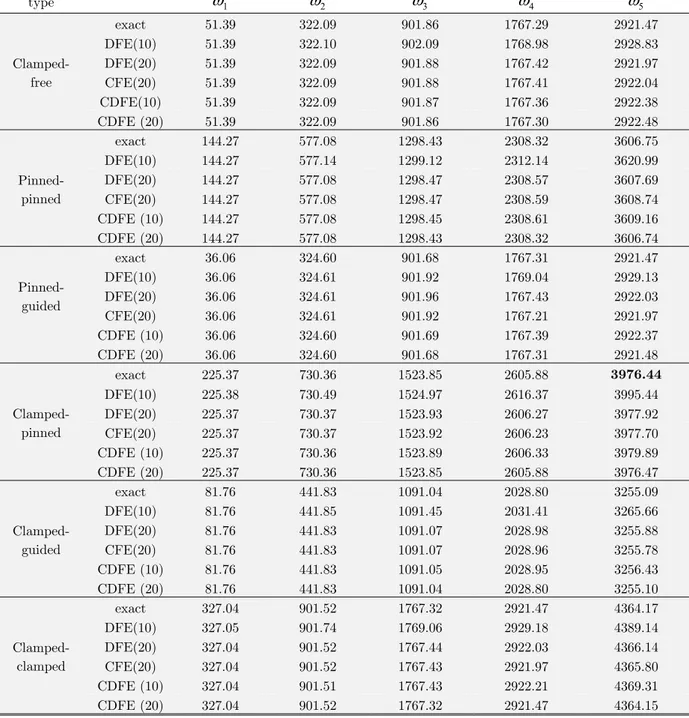
5 NUMERICAL EXAMPLES

In this section, some numerical examples are presented and the results are verified using DFE method. For this purpose, the beams in the presented examples are assumed to be made of steel bar of

0.1

m



0.1

m

rectangular cross section for which 7800 /kg m3 and E200 GPA. Also, the

length of the beam is considered to be 1 m.

type



1



2



3



4



5

Clamped-free

exact 51.39 322.09 901.86 1767.29 2921.47

DFE(10) 51.39 322.10 902.09 1768.98 2928.83

DFE(20) 51.39 322.09 901.88 1767.42 2921.97

CFE(20) 51.39 322.09 901.88 1767.41 2922.04

CDFE(10) 51.39 322.09 901.87 1767.36 2922.38

CDFE (20) 51.39 322.09 901.86 1767.30 2922.48

Pinned-pinned

exact 144.27 577.08 1298.43 2308.32 3606.75

DFE(10) 144.27 577.14 1299.12 2312.14 3620.99

DFE(20) 144.27 577.08 1298.47 2308.57 3607.69

CFE(20) 144.27 577.08 1298.47 2308.59 3608.74

CDFE (10) 144.27 577.08 1298.45 2308.61 3609.16

CDFE (20) 144.27 577.08 1298.43 2308.32 3606.74

Pinned-guided

exact 36.06 324.60 901.68 1767.31 2921.47

DFE(10) 36.06 324.61 901.92 1769.04 2929.13

DFE(20) 36.06 324.61 901.96 1767.43 2922.03

CFE(20) 36.06 324.61 901.92 1767.21 2921.97

CDFE (10) 36.06 324.60 901.69 1767.39 2922.37

CDFE (20) 36.06 324.60 901.68 1767.31 2921.48

Clamped-pinned

exact 225.37 730.36 1523.85 2605.88 3976.44

DFE(10) 225.38 730.49 1524.97 2616.37 3995.44

DFE(20) 225.37 730.37 1523.93 2606.27 3977.92

CFE(20) 225.37 730.37 1523.92 2606.23 3977.70

CDFE (10) 225.37 730.36 1523.89 2606.33 3979.89

CDFE (20) 225.37 730.36 1523.85 2605.88 3976.47

Clamped-guided

exact 81.76 441.83 1091.04 2028.80 3255.09

DFE(10) 81.76 441.85 1091.45 2031.41 3265.66

DFE(20) 81.76 441.83 1091.07 2028.98 3255.88

CFE(20) 81.76 441.83 1091.07 2028.96 3255.78

CDFE (10) 81.76 441.83 1091.05 2028.95 3256.43

CDFE (20) 81.76 441.83 1091.04 2028.80 3255.10

Clamped-clamped

exact 327.04 901.52 1767.32 2921.47 4364.17

DFE(10) 327.05 901.74 1769.06 2929.18 4389.14

DFE(20) 327.04 901.52 1767.44 2922.03 4366.14

CFE(20) 327.04 901.52 1767.43 2921.97 4365.80

CDFE (10) 327.04 901.51 1767.43 2922.21 4369.31

CDFE (20) 327.04 901.52 1767.32 2921.47 4364.15

Table 1: Natural frequencies of the different beam using CFE, CDFE and DFE methods.

Now, two examples for the static analysis of beams are presented. In the first example, deflec-tion, slope and curvature distribution of a simply support beam caring a uniformly distributed load

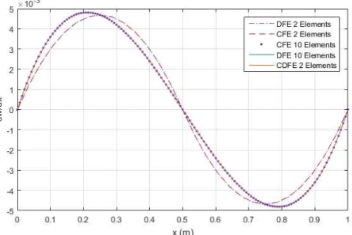
Figure 2: Deflection distribution of simply support beam using DFE, CFE and CDFE methods.

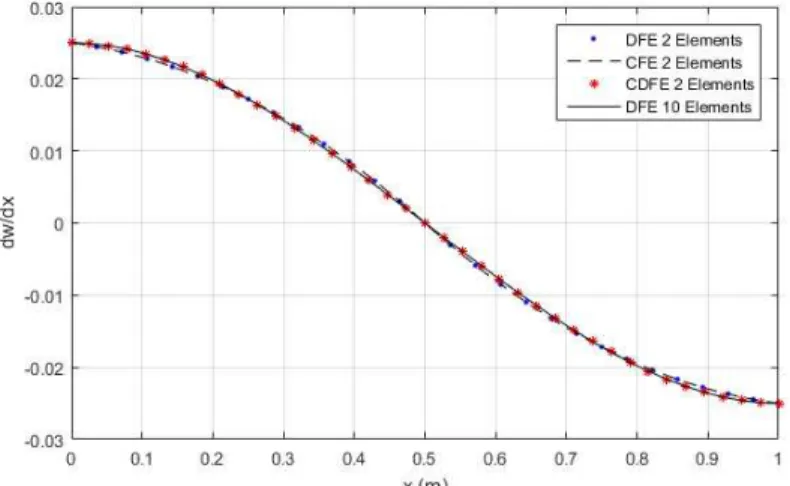
Figure 3: Slope distribution of simply support beam using DFE, CFE and CDFE methods.

For a clamped-clamped beam with uniformly distributed loadw 10 KN / m  , deflection, slope and its curvature distributions are plotted in Figures 5 to 7.

Figure 5: Deflection distribution of a clamped-clamped beam using DFE, CFE and CDFE methods.

Figure 6: Slope distribution of a clamped-clamped beam using DFE, CFE and CDFE methods.

It can be seen from Figures 2 to 7 that the deflection and slope distribution in the DFE, CFE and CDFE methods with two elements have the same accuracy. The curvature distribution in CDFE with two elements is close to the results of DFE method with ten elements which confirm the effectiveness of the CDFE method in comparison with DFE method.

Now, the dynamic response of an Euler-Bernoulli beam with CFE and CDFE methods are in-vestigated. In the first example, midpoint deflection of a clamped free beam under a suddenly ap-plied concentrated load w 10 KN at point x 3 4   is shown in Figure 8.

Figure 8: Midpoint deflection of a clamped-pined beam using CFE method.

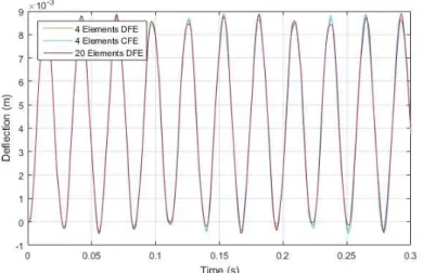
The second example is related to the dynamic response of a clamped free beam with a spring at its right end ( k 6000 KN / m  ). The deflection of the midpoint of the beam in the presence of a suddenly distributed uniform load w 10 KN / m  is depicted in Figure 9.

As can be seen, CFE and CDFE methods have the same accuracies in comparison with DFE method. Since the number of nodal variables in CFE and CDFE methods is less than that of DFE method, the computational cost is reduced. Thus, the proposed methods are more efficient for dy-namic analysis of beams and can be used for the dydy-namic analysis of different problems in solid mechanics.

6 CONCLUSION

This study focused on the dynamic analysis of Euler-Bernoulli beams using curvature and curvature derivative-based finite element methods. In curvature based finite element method (CFE) instead of interpolating displacement of Euler Bernoulli beam in usual displacement based finite element method (DFE), second derivative of displacement is interpolated. CFE method previously was used by a few researchers for dynamic analysis of clamped beams. In this research, CFE method was modified for static and dynamic analysis of beams with various boundary conditions.

In addition, a new method called CDFE (curvature derivative-based finite element) which is somehow a modification of CFE, was proposed. CDFE method, which interpolates the derivative of curvature instead of curvature, was used for beams with different boundary conditions.

The results were compared with those obtained by DFE method and the effectiveness of the CFE and CDFE methods was shown. In comparison with DFE method, the proposed methods have the following advantages:

 The bending moment in CFE method and the bending moment and the shear stress at the

internal nodes in CDFE method are continuous.

 With fewer numbers of elastic degrees of freedom, CFE and CDFE methods are more

accu-rate than DFE method.

References

Chen, Z., Kong, M., Ji, C., & Liu, M. (2015). An efficient dynamic modelling approach for high-speed planar parallel manipulator with flexible links. Proceedings of the Institution of Mechanical Engineers, Part C: Journal of Mechani-cal Engineering Science, 229(4), 663-678.

De Veubeke, B. F. (1965). Displacement and equilibrium models in the finite element method. Stress analysis, 9, 145-197.

De Veubeke, B. F., Zienkiewicz, O. C. (1967). Strain-energy bounds in finite-element analysis by slab analogy. Jour-nal of Strain AJour-nalysis, 2(4), 265-271.

Farid, M., & Cleghorn, W. L. (2014). Dynamic modeling of multi-flexible-link planar manipulators using curvature– based finite element method. Journal of Vibration and Control, 20(11), 1682-1696.

Farid, M., Cleghorn W. L. (2012). Dynamic Modeling of a Single-Flexible-Link Spatial Manipulator Using Curva-ture–Based Finite Element Method. Proceedings of the Canadian Society for Mechanical Engineering International Congress.

Kuo, Y. L. (2015). Stress-based Finite Element Analysis of Sliding Beams. Appl. Math, 9(2L), 609-616.

Kuo, Y. L., & Cleghorn, W. L. (2010). Curvature-and displacement-based finite element analyses of flexible four-bar mechanisms. Journal of Vibration and Control, 17(6), 827-844.

Kuo, Y. L., Cleghorn, W. L., & Behdinan, K. (2006). Stress-based finite element method for Euler-Bernoulli beams. Transactions of the Canadian Society for Mechanical Engineering, 30(1), 1-6.

Morley, L. S. D. (1968). The triangular equilibrium element in the solution of plate bending problems. Aeronautical Quarterly, 19(02), 149-169.

Punch, E.F., Atluri, S.N. (1986). Large displacement analysis of plates by stressed-based finite element approach. Computers and Structures, 24(1), 107-117.

Watwood, V. B., & Hartz, B. J. (1968). An equilibrium stress field model for finite element solutions of two-dimensional elastostatic problems. International Journal of Solids and Structures, 4(9), 857-873.

Wieckowski, Z. (1995). Dual finite element analysis for plasticity–friction torsion of composite bar. International journal for numerical methods in engineering, 38(11), 1901-1916.

Więckowski, Z., Youn, S. K., & Moon, B. S. (1999). Stress based finite element analysis of plane plasticity problems. International journal for numerical methods in engineering, 44(10), 1505-1525.

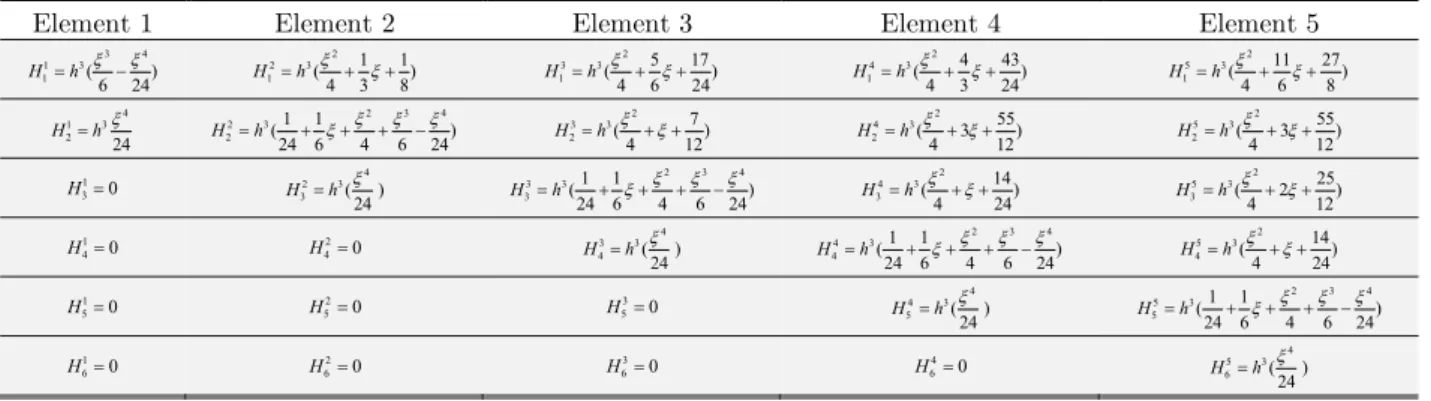
APPENDIX

The first five Shape functions of Euler-Bernoulli beam for CFE and CDFE methods are presented in the following table.

Element 1 Element 2 Element 3 Element 4 Element 5

2 3 1 2 1 (₂₆)

H h     ₁2 2(1 1)

2 3

 

H h    3 2

1 (1₂ 5₆)

H h    H14h2(1₂8₆)  H15h2(₂111₆)  3

1 2 2 ( )₆

H h    H22h2( 1)   H23h2( 1)   H42h2(2)  H52h2(3)  1

30

H  

3 2 2 3 ( )₆ H h   

2 3 3 2

3

1 1

( )

2 6 2 6

   

H h      H43h2( 1)   H35h2(2)  1

40

H   H₄20  3 2 3

4 ( )₆ H h   

2 3 4 2

4 (1₂  1_{6 2}₆)

H h      H45h2( 1)   1

50

H   H520  H530 

3 4 2 5 ( )₆ H h   

2 3 5 2

5 (1₂  1_{6 2}₆)

H h     

1 60

H   H620  H630  H460 

3 5 2 6 ( )₆ H h 

Table 2: Shape functions (CFE).

Element 1 Element 2 Element 3 Element 4 Element 5

3 1 3 1 4 ( ) 24 6  

H h    

2 2 3

1 (_{4 3}1 1₈)

H h    

2 3 3

1 (₄5₆ 17₂₄)

H h    

2 4 3

1 (₄₃4 43₂₄)

H h    

2 5 3

1 (₄11₆ 27₈)

H h    

1 3 2 4 24  H h  

4 2 3 2 3

2 (_{24 6}1 1 ₄_{6 24} )

H h      

2 3 3 2 (₄ ₁₂7)

H h    

2 4 3

2 (₄ 3 ₁₂55)

H h    

2 5 3

2 (₄ 3 ₁₂55)

H h    

1 30

H   2 3

3 4

( ) 24

 H h   

4 2 3 3 3

3 (_{24 6}1 1 ₄_{6 24} )

H h      

2 4 3 3 (₄ 14₂₄)

H h    

2 5 3

3 (₄ 2 ₁₂25)

H h    

1 40

H   H420  43 3

4

( ) 24

 H h   

4 2 3 4 3

4 (_{24 6}1 1 ₄_{6 24} )

H h      

2 5 3 4 (₄ 14₂₄)

H h    

1 50

H   H520  H350  54 3

4

( ) 24

 H h   

4 2 3 5 3 5 1 1 ( )

24 6 4 6 24

    

H h      

1 60

H   H620  H360  H640  56 3

4

( ) 24

 H h 