R-seqQI: RNA-Seq Quality Indicator

(1)

Universidade do Minho

Escola de Engenharia

Abel Ernesto Fernandes de Sousa

(2)

(3)

Universidade do Minho

Dissertação de Mestrado

Escola de Engenharia

Departamento de Informática

Abel Ernesto Fernandes de Sousa

R-seqQI: RNA-Seq Quality Indicator

Mestrado em Bioinformática

Trabalho realizado sob orientação de

Doutor Rui Mendes

Doutora Conceição Egas

Mestre Hugo Froufe

(4)

Declaração para efeitos de reprodução: Nome: Abel Ernesto Fernandes de Sousa

Título dissertação: R-seqQI: RNA-Seq Quality Indicator

Orientador(es): Rui Mendes PhD, Conceição Egas PhD, Hugo Froufe MSc Ano de conclusão: 2016

Designação do Mestrado: Mestrado em Bioinformática, Área de Especialização em Tecnologias de Informação

DE ACORDO COM A LEGISLAÇÃO EM VIGOR, NÃO É PERMITIDA A REPRODUÇÃO DE QUALQUER PARTE DESTA TESE/TRABALHO

Universidade do Minho, 31/01/2016

(5)

Agradecimentos

Antes de mais gostaria de agradecer ao meu orientador e à minha co-orientadora, Dr.º Rui Mendes e Dr.ª Conceição Egas, por todo o auxílio que me prestaram sempre que assim o solicitei. Quero também agradecer à pessoa que mais contactou comigo, o meu co-orientador Hugo Froufe, por toda a ajuda e acompanhamento que me deu ao longo desta jornada na Genoinseq. Todos aqueles brainstormings mostraram-se cruciais para o desenrolar deste estudo, e, sem ele, a sua concretização não teria sido possível. Fica também um muito obrigado à restante equipa da Genoinseq, pelo ambiente acolhedor que proporcionou durante esta estadia, e, em particular, ao técnico de Bioinformática Felipe Santos, por ter-se sempre prontificado em me esclarecer qualquer dúvida. Vou agora reservar um cantinho especial à aluna de Doutoramento Susana Margarida, ou, de um modo mais coloquial, à “sô dotora”. A ela o meu mais profundo obrigado por todos os bons momentos que passamos juntos, que foram imensos. Foi com ela que consegui espairecer e esquecer as frustrações, e sei que ficou uma grande, senão a minha maior, amiga. Não me querendo alongar mais, vou também agradecer aos meus pais e irmã, em muito, porque foram eles que me deram a possibilidade de realizar esta dissertação. Como um refúgio extra nos momentos de maior stress foram todos os meus amigos conterrâneos, que sempre me deram forças e ajudaram a descontrair quando assim necessitava. Não me poderei esquecer também dos meus grandes amigos de licenciatura, Luís Campos, Marco Queirós e Paulo Castro, que, apesar de ultimamente termos estado mais distantes por motivos académicos, sempre me deram confiança com prontidão. Por isso, a todos eles, o meu obrigado!

(6)

(7)

Abstract

The current progress of sequencing systems facilitates the sequencing of the genomes and transcriptomes of countless organisms on our planet. However, it is not simple to measure the quality of the processed data, mainly in the study of non-model organisms, for which there is little if any, information available. The Korf Lab developed a method for the evaluation of genomes integrity, through the identification of 248 core eukaryotic genes (CEGs) that are present in nearly all of the eukaryotes. The main goal of this work is to evaluate the use of the CEGs in RNA-Seq of non-model organisms. For that two software’s were developed: seqQIrefmetrics to calculate a set of reference-based quality metrics, including identification, chimerism, accuracy and contiguity, based on the literature, and three new metrics, comprising fragmentation(1,2,3,4,5+), coverage and non-match, increasing the number of metrics available for transcriptome quality assessment; and seqQIidentifyCEGs to identify and report the number of CEGs present in each transcriptome assembly. To carry out the main objective, RNA-Seq data from nine model organisms (Arabidopsis thaliana, Aspergillus nidulans, Caenorhabditis elegans, Drosophila melanogaster, Homo sapiens, Mus musculus, Oryza sativa, Saccharomyces cerevisiae and Xenopus tropicalis), processed with Trinity, were used to evaluate how CEG detection correlates with the quality of the transcriptomes. In order to identify CEGs, protein sequences from assembled transcripts were predicted with TransDecoder. Metrics calculated by seqQIrefmetrics were associated with the number of CEGs identified by seqQIidentifyCEGs in each assembled transcriptome, through linear regressions. Among these metrics only contiguity and coverage were used to create predictive models, achieving an R2 of 0.787 and 0.640; and a RMSE of

5.86 and 6.90, respectively. These findings indicate that the CEGs can be used as a quality tool. In fact, the linear regressions enable to infer prospectively the quality of the assembled transcripts, without the necessity of additional information, such as a reference genome sequence or structural annotations. This approach is extremely important for RNA-Seq of non-model organisms, where there is no such information to evaluate the quality of the assembled transcripts in a reliable manner.

(8)

(9)

Resumo

Os progressos nas plataformas de sequenciação atuais permitem a obtenção dos genomas e transcritomas dos inúmeros organismos que habitam o nosso planeta. Contudo, não é simples avaliar a qualidade dos dados já processados, principalmente em estudos de organismos não modelo, para os quais existe pouca, se alguma, informação disponível. O grupo de investigação “The Korf Lab” desenvolveu um método para avaliar a integridade de sequências genómicas, através da identificação de 248 “core eukaryotic genes” (CEGs) que são conservados nos eucariontes. O principal objetivo deste trabalho é avaliar a utilização dos CEGs em RNA-Seq de organismos não modelo. De modo a atingir este objectivo dois softwares foram desenvolvidos: seqQIrefmetrics, para calcular um conjunto de métricas baseadas em referência, incluindo “identification”, “chimerism”, “accuracy” e “contiguity”, com base na literatura, e três novas métricas, “fragmentation(1,2,3,4,5+)”, “coverage” e “non-match”, aumentando assim o numero de métricas disponíveis para a avaliação da qualidade de transcritomas; e seqQIidentifyCEGs para identificar e reportar o número de CEGs presentes em cada transcritoma. Os dados de RNA-Seq de nove organismos modelo (Arabidopsis thaliana, Aspergillus nidulans, Caenorhabditis elegans, Drosophila melanogaster, Homo sapiens, Mus musculus, Oryza sativa, Saccharomyces cerevisiae e Xenopus tropicalis), processados com o Trinity, foram usados para avaliar como a detecção dos CEGs se correlaciona com a qualidade dos transcritomas. De modo a identificar os CEGs, as sequências proteicas dos transcritos assemblados foram determinadas com o TransDecoder. As métricas calculadas com seqQIrefmetrics foram associadas com o número de CEGs identificados com seqQIidentifyCEGs, em cada transcritoma assemblado, através de regressões lineares. Entre estas métricas apenas “contiguity” e “coverage” foram usadas para criar modelos preditivos, atingindo um R2 de 0,787 e 0,640; e um RMSE de 5,86 e 6,90, respetivamente. Estes

resultados sugerem que os CEGs poderão ser usados como uma ferramenta de qualidade. Na verdade, as regressões lineares permitem inferir a qualidade dos transcritos assemblados, sem a necessidade de informação adicional, como um genoma de referência ou anotações estruturais. Este

(10)

método é assim extremamente importante para estudos de RNA-Seq de organismos não modelo, onde não existe tal informação que permita avaliar a qualidade dos transcritos de um modo viável.

(11)

5. Methodologies ... 39 5.1. Brief overview ... 39 5.2. Data sets ... 40 5.3. Quality control ... 41 5.4. Implemented assemblies ... 42 5.4.1. Reference-based ... 42 5.4.2. de novo ... 43 5.5. Quality metrics ... 43 5.6. CEGs identification ... 44 5.7. Models development ... 45 6. Code implementation ... 47 6.1. seqQIrefmetrics ... 47 6.1.1. Overview ... 47

6.1.2. Input files and procedures ... 53

6.2. seqQIidentifyCEGs ... 59

6.2.1. Overview ... 59

(13)

7. Results and discussion ... 63

7.1. Data sets ... 63

7.2. Quality control checks ... 64

7.3. Assemblies ... 65

7.4. Reference-based quality metrics results ... 67

7.4.1. Reference-based assembled transcriptomes ... 68

7.4.2. de novo assembled transcriptomes ... 71

7.5. Quality metrics and CEGs: models establishment ... 74

7.5.1. Coverage model ... 80

7.5.2. Contiguity model ... 82

8. Conclusions and future work ... 87

8.1. Summary ... 87 8.2. Future work ... 88 References ... 89 Supplementary material ... 103 Appendix A ... 103 Appendix B ... 110 Appendix C ... 111

(14)

(15)

List of figures

Figure 1 - Tridimensional view of the DNA molecule. The DNA molecule is composed by two polynucleotide strands arranged in a double helix, stabilized by hydrogen bonds between the nucleotide bases: adenine (A) forms two hydrogen bonds with thymine (T) and cytosine (C) forms three hydrogen bonds with guanine (G). The arrows reflect the antiparallel relation between the polynucleotide strands. Adapted from (Alberts et al., 2010). ... 6 Figure 2 - Eukaryotic genome and gene structure. The eukaryotic genome is organized in intergenic (non-coding) and genic (coding) regions. Genes comprise the coding region. This figure illustrates the promoter, responsible for controlling the initiation of transcription with the CpG Island; the transcription start site; the exons (coding regions) and introns (non-coding segments); the donor and acceptor sites used to splice exons on both sides of an intron in a process known as splicing; the 5’ and 3’ untranslated regions (UTR’s). These regions are important in the regulation of translation; the initial and final exons with the corresponding start and stop codons; and the poly-A site. Adapted from (Akhtar et al., 2008). ... 8 Figure 3 - Simplified representation of the central dogma of molecular biology. mRNA is synthesized from DNA by a process called transcription. The information carried by mRNA is then translated into proteins, which make up the structure of cells and are responsible for most of its functions. Translation occurs in ribosomes with the intervention of two other types of RNA molecules: transfer RNA (tRNA) and ribosomal RNA (rRNA). tRNA transports the amino acids to the growing polypeptide chain and rRNA is a component of ribosomes. ... 9 Figure 4 - Alternative splicing event. Eukaryotic pre-mRNAs are composed of exons (coding sequences) and introns (non-coding sequences). Three regions are extremely important during the process of splicing: splice-donors, branch sites, and splice-acceptors. During splicing, the exons can be joined in different combinations, yielding different mRNA molecules, called isoforms. This process is called alternative splicing and enables a single gene to express different proteins. ... 12

(16)

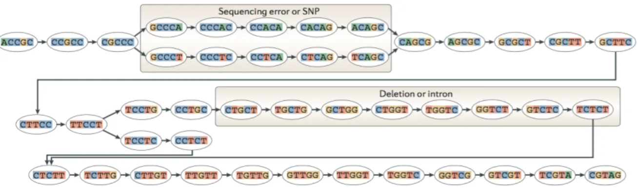
Figure 5 - The genetic code. This table contains the 64 codons that constitute the genetic code. In order to be read the first letter in the left column should be selected, followed by the second letter in the top row and the third letter in the right column. The names of the amino acids are abbreviated. Adapted from (Hartwell et al., 2011h). ... 13 Figure 6 - TopHat pipeline. Initially, the reads are mapped to the genome sequence, and the IUM reads are collected. After assembling the covered regions in a consensus sequence and searching for the potential splice junctions, the IUM reads are aligned to these regions via a seed-and-extend algorithm. Adapted from (Trapnell et al., 2009). ... 19 Figure 7 - MMP search detecting a splice junction. The RNA-Seq read here illustrated cannot be contiguously mapped to the genome, because it aligns to a splice junction. Therefore, the first MMP was mapped to a donor splice site. The second MMP search is repeated for the unmapped portion of the read, which, in this case, was mapped to an acceptor splice site. Adapted from (Dobin et al., 2013). ... 20 Figure 8 - De Bruijn graph. The construction of a De Bruijn Graph starts with the generation of all

k-mers with length k (5 in this example) from the reads. Then they are integrated into a De Bruijn Graph and two k-mers are connected if they share an overlap equal to k-1. The existence of sequencing errors or SNPs (A/T) and also introns or deletions between the reads introduces alternative paths through the graph, which can be traversed by specific algorithms to recover the most probable transcripts sequences. Adapted from (Martin and Wang, 2011). ... 22 Figure 9 - Trinity assembly pipeline. Inchworm constructs contigs using the k-mers generated by Jellyfish. Then, Chrysalis builds clusters of related Inchworm contigs, and each one is processed into a De Bruijn graph. Finally, Butterfly extracts all probable transcripts from each graph. Adapted from (Haas et al., 2013). ... 23 Figure 10 - Expression level estimation by RSEM. RSEM integrates the EM algorithm to estimate the transcripts abundances. In this example two different isoforms (long bars) are represented, containing portions of shared (blue) and unique (red and yellow) sequences. The reads (short bars) are initially aligned to the transcripts sequences, and the unique regions of isoforms will capture uniquely mapping reads (red and yellow short bars), while the shared sequences will be the target of multiply mapping reads. The EM algorithm estimates the relative abundances of the transcripts, and then fractionally assigns reads to the isoforms based on these abundances. This assignment occurs iteratively, represented as filled short bars (right). The eliminated assignments

(17)

correspond to the hollow bars. Finally, a higher fraction of each read is assigned to the top isoform (highly expressed) than to the bottom isoform. Adapted from (Haas et al., 2013). ... 24 Figure 11 - Methodologies overview. Blue - source of the data sets; gray - data sets; orange - data processing. ... 40 Figure 12 - Identification metric. One assembled transcript identifies the reference transcript A, while two assembled transcripts identify the reference transcript B. The reference transcript C is not identified. ... 48 Figure 13 - Contiguity metric. The reference transcript identified A is covered above 80% of its size, by a single assembled transcript. ... 48 Figure 14 – Fragmentation(1,2,3,4,5+) metric. The reference transcript identified A is covered below 80% of its size, by a single assembled transcript, while the reference transcripts identified B, C, D and E are covered by two, three, four and five or more (dots) assembled transcripts, respectively. ... 49 Figure 15 - Coverage metric. The reference transcripts identified A, B and C have a coverage percentage of 90%, 50% and 30%, of their size, respectively. The coverage of transcripts A, B and C correspond therefore to (90 + 50 + 30) ÷ 3 ≈ 57%. ... 50 Figure 16 - Accuracy metric. The alignment between the reference transcript identified A and the assembled transcript B has 18 matches (equal bases), one mismatch (red) and three gaps (blue), yielding an alignment with 22 bp. The accuracy of the transcript B assembly, in particular, corresponds to 18 ÷ 22 ≈ 82%. ... 51 Figure 17 - Chimerism metric. The assembled transcript A contains two reference transcripts aligned in distinct regions. ... 52 Figure 18 - Non-match metric. The assembled transcript A does not match with any reference transcript. The assembled transcript B matches with a reference transcript, but the coverage percentage of assembled transcript B is lower than 80% of its size. ... 52 Figure 19 - Command-line interface for seqQIrefmetrics.py. This interface explains how to execute seqQIrefmetrics and shows the parameters that are available to the user. ... 54 Figure 20 - Complete and partial overlaps between assembled transcripts. i1/f1 – initial and final positions of the alignment of the first assembled transcript (largest); i2/f2 – initial and final positions of the alignment of the second assembled transcript (smallest); A – The reference transcript contains two assembled transcripts establishing a complete overlap, so that the shared region encompasses the entire size of the small assembled transcript (i2 > i1 and f2 < f1); i3/f3

(18)

– initial and final positions of the alignment of the third assembled transcript; i4/f4 – initial and final positions of the alignment of the fourth assembled transcript; B – the reference transcript contains two assembled transcripts establishing a partial overlap, so that the final position of the fourth assembled transcript (f4) is higher than the final position of the third assembled transcript (f3), and the initial position of the fourth assembled transcript (i4) is lower than the final position of the third assembled transcript (f3). The coverage of reference transcript B is determined between the initial (i3) and final (f4) positions of the third and fourth overlapped assembled transcript. ... 56 Figure 21 - Metrics results for the reference-based assembled transcriptome of Saccharomyces cerevisiae (100% of the data). The number of reference, assembled and expressed transcripts are initially reported, with the coverage thresholds. The metrics results and the number of assembled transcripts used are then reported, with the time required for the calculations (in hours, minutes and seconds). ... 58 Figure 22 - Metrics results for the de novo assembled transcriptome of Saccharomyces cerevisiae (100% of the data). The number of reference, assembled and expressed transcripts are initially reported, with the coverage thresholds. The metrics results and the number of assembled transcripts used are then reported, with the time required for the calculations (in hours, minutes and seconds). ... 58 Figure 23 - Command-line interface for seqQIidentifyCEGs.py. This interface explains how to execute seqQIidentifyCEGs.py and shows the parameters that are available to the user. ... 60 Figure 24 - Number of CEGs identified for the reference-based assembled transcriptome of Saccharomyces cerevisiae (100% of the data). Total number of CEGs identified with the respective number by conservation group (1-4). ... 62 Figure 25 - Number of CEGs identified for the de novo assembled transcriptome of Saccharomyces cerevisiae (100% of the data). Total number of CEGs identified with the respective number by conservation group (1-4). ... 62 Figure 26 - Scatterplot of the percentage of fragmentation(1,2,3,4,5+) vs the number of CEGs (group A). Blue – fragmentation(1); red - fragmentation(2); green - fragmentation(3); purple - fragmentation(4); yellow - fragmentation(5+). ... 79 Figure 27 - Scatterplot of the percentage of coverage vs. the number of CEGs identified (group A). The intercept and slope of the regression line correspond to 37.151 and 0.368, respectively. ... 80

(19)

Figure 28 - Scatterplot of the residuals vs. the predicted percentages of coverage. The residuals of the coverage prediction model show a random pattern, indicating a good fit for a linear model. ... 81 Figure 29 - Scatterplot of the percentage of contiguity vs. the number of CEGs identified (group A). The intercept and slope of the regression line correspond to -11.135 and 0.563, respectively. ... 82 Figure 30 - Scatterplot of the residuals vs. the predicted percentages of contiguity. The residuals of the contiguity prediction model do not show a random pattern (U-shaped), indicating a better fit for a non-linear model. ... 83 Figure 31 - Scatterplot of the log transformed contiguity vs. the number of CEGs identified (group A). The intercept and slope of the regression line correspond to 0.694 and 0.009, respectively. ... 84 Figure 32 - Scatterplot of the residuals vs. the predicted contiguity (log). The residuals of the log transformed contiguity model show a random pattern, suggesting that the transformation to achieve linearity was successful. ... 85 Figure 33 - Per base sequence quality overview of the raw reads of A. thaliana, A. nidulans and C. elegans extracted from FASTQC. Overview of the range of quality values, across all bases at each read position, for the left (left graphs) and right (right graphs) reads of the pairs. The blue and red lines are the mean and median values, respectively. The background is divided into very good quality calls (green), calls of reasonable quality (orange) and calls of poor quality (red). ... 104 Figure 34 - Per base sequence quality overview of the raw reads of D. melanogaster, H. sapiens and M. musculus extracted from FASTQC. Overview of the range of quality values, across all bases at each read position, for the left (left graphs) and right (right graphs) reads of the pairs. The blue and red lines are the mean and median values, respectively. The background is divided into very good quality calls (green), calls of reasonable quality (orange) and calls of poor quality (red). ... 105 Figure 35 - Per base sequence quality overview of the raw reads of O. sativa, S. cerevisiae and X. tropicalis extracted from FASTQC. Overview of the range of quality values, across all bases at each read position, for the left (left graphs) and right (right graphs) reads of the pairs. The blue and red lines are the mean and median values, respectively. The

(20)

background is divided into very good quality calls (green), calls of reasonable quality (orange) and calls of poor quality (red). ... 106 Figure 36 - Per base sequence quality overview of the filtered reads of A. thaliana, A. nidulans and C. elegans extracted from FASTQC. Overview of the range of quality values, across all bases at each read position, for the left (left graphs) and right (right graphs) reads of the pairs. The blue and red lines are the mean and median values, respectively. The background is divided into very good quality calls (green), calls of reasonable quality (orange) and calls of poor quality (red). ... 107 Figure 37 - Per base sequence quality overview of the filtered reads of D. melanogaster, H. sapiens and M. musculus extracted from FASTQC. Overview of the range of quality values, across all bases at each read position, for the left (left graphs) and right (right graphs) reads of the pairs. The blue and red lines are the mean and median values, respectively. The background is divided into very good quality calls (green), calls of reasonable quality (orange) and calls of poor quality (red). ... 108 Figure 38 - Per base sequence quality overview of the filtered reads of O. sativa, S. cerevisiae and X. tropicalis extracted from FASTQC. Overview of the range of quality values, across all bases at each read position, for the left (left graphs) and right (right graphs) reads of the pairs. The blue and red lines are the mean and median values, respectively. The background is divided into very good quality calls (green), calls of reasonable quality (orange) and calls of poor quality (red). ... 109

(21)

List of tables

Table 1 - Current-sequencing platforms. Seller and respective instrument, with the run time in hours, mean of read length, reads per run in millions, yield per run (Gb, billion of bases and Mb, million of bases) and cost per run and Mb. The indicated prices concern the sequencing reaction reagents and do not include library preparation reagents, labor, data storage or analysis, equipment or maintenance. Adapted from (Li et al., 2014b). ... 2 Table 2 - BLAST programs. The BLAST consists of several utilities, each one with a specific query and target type. For example, BLASTP compares an amino acid query sequence against a protein sequence database. ... 27 Table 3 - Information of the data sets for each organism. Accession number, read length, sequencing technology, genome version and number of reference transcripts for each organism. ... 63 Table 4 - Number of raw and filtered reads for each organism. Number of filtered reads, using PRINSEQ, from the raw data sets downloaded from NCBI SRA (for A. thaliana, A. nidulans, C. elegans, O. sativa, S. cerevisiae and X. tropicalis) and ENCODE (for D. melanogaster, H.sapiens and M. musculus). ... 65 Table 5 - Number of assembled and expressed transcripts for both assembly strategies across the three sequencing libraries. The N50 length is also indicated. A.t – assembled transcripts; E.t. - expressed transcripts (FPKM > 0). ... 66 Table 6 - Metrics results for the reference-based assembled transcriptomes across the three sequencing libraries. Id. - identification; Cov. - coverage; Cont. - contiguity; N.m. - non-match; Ch. - chimerism. ... 69 Table 7 - Fragmentation results for the reference-based assembled transcriptomes across the three sequencing libraries. Frag(1) - Frag(4): reference transcripts aligning with one to four assembled transcripts; Frag(5+): reference transcripts aligning with five or more assembled transcripts. ... 71

(22)

Table 8 - Metrics results for the de novo assembled transcriptomes across the three sequencing libraries. Id. - Identification; Cov. - coverage; Cont. - contiguity; N.m. - non-match; Ch. - chimerism. ... 72 Table 9 - Fragmentation results for the de novo assembled transcriptomes across the three sequencing libraries. Frag(1) - Frag(4): reference transcripts aligning with one to four assembled transcripts; Frag(5+): reference transcripts aligning with five or more assembled transcripts. ... 73 Table 10 - Number of CEGs identified for both assembly strategies across the three sequencing libraries. Total - total number of CEGs identified; Group A - number of CEGs identified of conservation levels 1 and 2; Group B - number of CEGs identified of conservation levels 3 and 4. ... 75 Table 11 - Lilliefors Kolmogorov-Smirnov test. P-values of the Lilliefors Kolmogorov-Smirnov test, used to test the normality of the data. ... 76 Table 12 – Summary statistics for each linear regression. r - Pearson correlation coefficient, R2 - coefficient of determination and P-value of the T-test. ... 77

Table 13 - Accuracy results for the reference-based and de novo assembled transcriptomes across the three sequencing libraries. Percentage of correct bases in the assembled transcripts comparatively with the reference transcripts. ... 110 Table 14 - Summary statistics for each linear regression with the log transformation of each metric. r - Pearson correlation coefficient, R2 - coefficient of determination and P-value of

(23)

Acronyms

A Adenine

BAM Binary alignment/map format BeT Genome-specific best hit BLAST Basic local alignment search BLASTN Nucleotide BLAST

BLASTP Protein BLAST BLASTX Translated BLAST bp Base pairs C Cytosine

cDNA Complementary DNA CEGs Core eukaryotic genes

CEGMA Core eukaryotic genes mapping approach CentOS Community enterprise operating system COG Clusters of orthologous groups of proteins CPU Central processing unit

DNA Deoxyribonucleic acid dUTP Deoxyuridine triphosphate

EM Expectation-maximization algorithm ENCODE Encyclopedia of DNA elements EST Expression sequence tag

FPKM Fragments per kilobase of exon per million reads mapped G Guanine

GC Guanine and cytosine percentage GTF General transfer format

H0 Null hypothesis

(24)

HGP Human genome project HMMs Hidden Markov models

HMMER Hidden Markov model-based sequence alignment tool HSP High-scoring segment pairs

IsoPct Isoform expression percentage IUM Initially unmapped reads KOG Eukaryotic orthologous groups Ler Landsberg erecta

miRNA Micro RNA

MMP Maximal mappable prefix mRNA Messenger RNA

NCBI National Center for Biotechnology Information NGS Next-generation sequencing

ORF Open-reading frame PacBio Pacific Biosciences

PCR Polymerase Chain Reaction Pfam Protein families database PGM Personal genome machine pre-mRNA pre-messenger RNA

r Pearson correlation coefficient R2 Coefficient of determination

RABT Reference annotation based transcript assembly RAM Random-access memory

RISC RNA-induced silencing complex RITS RNA-induced transcriptional silencing RMSE Root-mean-square error

RNA Ribonucleic acid RNA-Seq RNA sequencing RNAi RNA interference rRNA Ribosomal RNA

RSEM RNA-Seq by expectation maximization RT-qPCR Reverse transcription quantitative PCR

(25)

SAM Sequence alignment/map format SNP Single nucleotide polymorphism snRNA Small nuclear ribonucleic acid snRNP Small nuclear ribonucleic proteins SRA Sequence read archive

STAR Spliced transcripts alignment to a reference T Thymine

T-coffee Tree-based consistency objective function for alignment evaluation TBLASTN Translated BLAST

TBLASTX Translated BLAST TPM Transcripts per million

Trans-ABySS Transcriptome assembly by short sequences tRNA Transfer RNA

U Uracil

UniProt Universal Protein Resource UTR Untranslated regions

(26)

(27)

1. Introduction

1.1. Context and motivation

The Human Genome Project (HGP) started in 1990, and it was a 13-year-long effort to obtain the first human genome sequence, costing a total of $3 billion over this period. The HGP was accomplished with first-generation sequencing equipment or Sanger sequencing (Sanger et al., 1977), a chain-termination method developed in 1975 by Edward Sanger. The conclusion of the HGP encouraged the development of cheaper and faster sequencing methods, resulting in the establishment of the second-generation sequencing, or next-generation sequencing (NGS), technologies. NGS platforms perform massively parallel sequencing, during which millions of fragments of DNA from a single sample are sequenced in parallel, allowing an entire genome to be sequenced in less than one day. In the past decade, several NGS platforms have been developed that provide low-cost, high-throughput sequencing, and some of the current technologies are described in Table 1. The NGS has countless applications in the biological research fields. In health, NGS enables to re-sequence the human genome to identify genes and regulatory elements involved in pathological processes, and also the sequencing of bacterial and viral organisms to identify novel virulence agents. Furthermore, gene expression studies or transcriptome analysis using NGS, or RNA sequencing (RNA-Seq), have begun to replace older methods such as microarrays, providing opportunities for multidimensional examinations of transcriptomes, in which high-throughput expression data are obtained at a single-base resolution (Grada and Weinbrecht, 2013).

(28)

Table 1 - Current-sequencing platforms. Seller and respective instrument, with the run time in hours, mean of read length, reads per run in millions, yield per run (Gb, billion of bases and Mb, million of bases) and cost per run and Mb. The indicated prices concern the sequencing reaction reagents and do not include library preparation reagents, labor, data storage or analysis, equipment or maintenance. Adapted from (Li et al., 2014b).

Company Instrument time Run (hours) Read length (mean) Reads per run (millions) Yield per run Cost per run ($) Cost per Mb ($) Illumina _2000/2500HiSeq 132 50 6,000 300 _Gb 18,725.00 0.06 Illumina MiSeq 39 250 30 7.5 _Gb 982,75 0.13 Life technologies PGM 7.3 176 6 1.056 Gb 749.00 0.71 Life technologies Proton 2-4 81 70 5.67 Gb 834.00 0.15 Pacific Biosciences RS 0.5-2 1,289 0.03 38.67 Mb 136.38 3.53 Roche 454 20 686 1 686 _Mb 5,985.00 8.72

The current progress of sequencing systems facilitates, therefore, the sequencing of the genomes and transcriptomes of countless organisms on our planet. However, it is not simple to measure the quality of the processed data. The Korf Lab developed a method for the evaluation of genomes integrity, through the identification of 248 core eukaryotic genes (CEGs) that are present in nearly all of the eukaryotes (Parra et al., 2009), in such a way that the number of CEGs present in the assemblies mirrors the quality and overall utility of the genome sequences. Regarding the transcriptomic assemblies, a set of metrics already published (Martin and Wang, 2011) enables to evaluate their quality, but it can only be applied for well-studied organisms due to the need for a reference genome and structural annotations, preventing the use in non-model species, for which there is little, if any, information available.

1.2. Objectives

The main goal of this master thesis is to evaluate the core eukaryotic genes (CEGs) as a quality control tool for RNA-Seq of non-model organisms. The utilization of the CEGs as a tool to evaluate the quality of these transcriptomes is important since the quality metrics previously mentioned rely on a set

(29)

of reference transcripts, which is not available for non-model organisms. In order to achieve this goal the following specific objectives were set up:

o Review the state-of-the-art and relevant concepts for the later steps.

o Obtain RNA-Seq sequencing data from model organisms and process the data using two different strategies.

o Develop a set of reference-based quality metrics and evaluate de novo and reference-based strategies based on these metrics.

o Develop a tool to survey the CEGs in the transcriptomic assemblies.

o Evaluate the relationship between the CEGs and the reference-based quality metrics through linear regressions.

o Establish quality predictive models.

1.3. Organization of the contents

Chapter 2. Fundamentals of genetics

Comprehensive review of the genetic foundations that underlie the living beings, with emphasis on the main mechanisms and molecules involved.

Chapter 3. Transcriptomics

Enlightenment of the transcriptomics object of study, along with its concepts and main methodologies will be described.

Chapter 4. Evolutionary genomics and genome annotation

The evolutionary genomics as a valuable key for genome annotation, and the main steps that led to the development and construction of the core eukaryotic genes.

Chapter 5. Methodologies

The required data processing will be described. Chapter 6. Code implementation

(30)

The description of the algorithms used to develop the necessary tools. Chapter 7. Results and discussion

The results obtained by the reference-based quality metrics and by the survey of the CEGs in the reconstructed transcriptomes. The results of the linear regressions conducted between these two variables will also be addressed.

Chapter 8. Conclusions and future work

(31)

2. Fundamentals of genetics

2.1. DNA as the source of biological information

The organisms now inhabiting the earth descended from a Last Universal Common Ancestor that lived approximately 3 billion years ago (Glansdorff et al., 2008). This evolutionary process is the result of amazingly efficient mechanisms to store, replicate, express and diversify biological information. In fact, all organisms, from bacteria and protozoa to more complex living beings, such as plants and animals, use vast quantities of information to develop and survive in their environments. These organisms must transmit their information to the next generations, ensuring the genetic continuity of each species. This biological information is encoded in a molecule called deoxyribonucleic acid, called DNA, and expressed in the form of proteins, with many functions in an organism including structural proteins, which make up the cellular compartments; motor proteins, which, as the name implies, are involved in the cellular movement; transport proteins, which carry materials across biological membranes; regulatory proteins, which control protein and gene function; and signaling proteins, that receive and process signals to initiate a physiological response (Hartwell et al., 2011f; Lodish et al., 2003j).

2.2. Structure and organization of DNA

DNA structure was published in 1953 by James Watson and Francis Crick (WATSON and CRICK, 1953). They determined that DNA consists of two antiparallel complementary strands of nucleotides, twisted around each other to form a right-handed double helix, held in place by hydrogen bonds between complementary base pairs: adenine pairs with thymine (A / T) and guanine pairs with cytosine (G / C). The structure of the DNA molecule can be seen in Figure 1. Each nucleotide is

(32)

composed of a deoxyribose sugar, a phosphate group, and a nitrogenous base, which, as noted, can vary among four kinds. The nucleotides are covalently linked in a polynucleotide chain through the phosphate groups, in which the 5’-phosphate group of one nucleotide is joined to the 3’-hydroxyl group of the next nucleotide, creating a phosphodiester bond. The addition of nucleotides is performed from the position 5’ to the position 3’ of the strand (5’ - 3’) (Nelson and Cox, 2008a).

Figure 1 - Tridimensional view of the DNA molecule. The DNA molecule is composed by two polynucleotide strands arranged in a double helix, stabilized by hydrogen bonds between the nucleotide bases: adenine (A) forms two hydrogen bonds with thymine (T) and cytosine (C) forms three hydrogen bonds with guanine (G). The arrows reflect the antiparallel relation between the polynucleotide strands. Adapted from (Alberts et al., 2010).

The biological information stored in DNA is organized in hereditary units called genes. These segments of DNA contain the information required for the synthesis of a biological product (protein or RNA) and determine the characteristics of an organism: its appearance and how it behaves and survives in its environment (Lodish et al., 2003a). DNA molecules carrying genes are organized in chromosomes, structures that package and manage the storage and expression of DNA. The entire collection of chromosomes in an organism is its genome (Hartwell et al., 2011g).

(33)

2.2.1. Structure of genes and genomes in prokaryotes

The genome of prokaryotes is usually organized in a single chromosome with a circular DNA molecule (Lodish et al., 2003b; Hartwell et al., 2011i). Other DNA molecules are also present, called plasmids. These smaller molecules can replicate independently of the main chromosome and confer resistance to toxins and antibiotics in the environment. Plasmids are especially prone to experimental manipulation and are powerful tools for genetic engineering and recombinant DNA technology (Cooper and Hausman, 2007a; Nelson and Cox, 2008c). On prokaryotes, genomes have few noncoding regions, and genes are very closely packed and arranged in operons, specialized in specific metabolic functions (Lodish et al., 2003c).

2.2.2. Structure of genes and genomes in eukaryotes

The genomes of eukaryotes are larger and more complex than those of prokaryotes. Much of the complexity results from the abundance of several different types of noncoding sequences (or intergenic regions), which constitute a large fraction of the genomes of higher eukaryotes. Eukaryotic genomes are also organized in multiple chromosomes, each containing a linear molecule of DNA bound to small proteins, histones, comprising a structure called chromatin. Histones are extremely important in the storage of DNA in the cell nucleus and are involved in a range of activities, including DNA replication and gene expression (Cooper and Hausman, 2007f). Unlike prokaryotes, eukaryotic genes involved in a single pathway are often physically separated in the DNA, even located on different chromosomes. Large amounts of noncoding sequences are found inside of most eukaryotic genes. Such genes are structured in pieces of coding sequences, the exons, separated by noncoding segments, the introns. These noncoding segments are extremely rare in prokaryotes and uncommon in many unicellular eukaryotes such as Saccharomyces cerevisiae (Lodish et al., 2003d; Cooper and Hausman, 2007g). The genomic and genic structure in eukaryotes is represented in Figure 2.

(34)

Figure 2 - Eukaryotic genome and gene structure. The eukaryotic genome is organized in intergenic (non-coding) and genic (coding) regions. Genes comprise the coding region. This figure illustrates the promoter, responsible for controlling the initiation of transcription with the CpG Island; the transcription start site; the exons (coding regions) and introns (non-coding segments); the donor and acceptor sites used to splice exons on both sides of an intron in a process known as splicing; the 5’ and 3’ untranslated regions (UTR’s). These regions are important in the regulation of translation; the initial and final exons with the corresponding start and stop codons; and the poly-A site. Adapted from (Akhtar et al., 2008).

2.3. An overview of gene expression

In any organism, genes specify the amino acid sequence of every protein, and, therefore, the kinds of proteins that are synthesized. However, the information encoded in DNA is not directly used for protein synthesis. There is a molecule that transports that information, acting as an intermediary. This molecule is the ribonucleic acid (RNA) and it is synthesized from DNA by a process called transcription. RNA molecules that carry the information encoded in DNA for protein synthesis are called messenger RNA (mRNA). Translation follows transcription, which is the actual synthesis of proteins according to the information in mRNA, with the intervention of other RNA molecules: transfer RNA (tRNA) translates the information in mRNA into a specific sequence of amino acids, and ribosomal RNA (rRNA) is a component, alongside proteins, of ribosomes, the protein complexes where translation occurs (Berg et al., 2002a; Nelson and Cox, 2008b).

(35)

The flow of genetic information depicted here was called the central dogma of molecular biology (Crick, 1970), which is illustrated in Figure 3. However, the simplified representation of the central dogma as a straightforward process from DNA to protein, having mRNA as an intermediary, does not reflect the role of proteins and even RNA in regulating gene expression (Lodish et al., 2003a; Berg et al., 2002b). As a matter of fact, the behavior of cells and their capacity to adapt to changes in their environments are determined not only by their genes but also by which of those genes are expressed at any given time, which in turn is determined by regulatory events (Cooper and Hausman, 2007b).

Figure 3 - Simplified representation of the central dogma of molecular biology. mRNA is synthesized from DNA by a process called transcription. The information carried by mRNA is then translated into proteins, which make up the structure of cells and are responsible for most of its functions. Translation occurs in ribosomes with the intervention of two other types of RNA molecules: transfer RNA (tRNA) and ribosomal RNA (rRNA). tRNA transports the amino acids to the growing polypeptide chain and rRNA is a component of ribosomes.

2.4. Transcription

Transcription consists in the polymerization of ribonucleotides (monomers of RNA) directed by complementary base pairing with the template strand of DNA that composes the gene. Transcription of DNA in prokaryotes and eukaryotes follows the same basic steps: initiation, elongation, and termination. Primarily, the enzyme responsible for catalyzing RNA synthesis, the RNA polymerase, binds to a DNA sequence at the beginning of the gene that controls the initiation of transcription: the promoter. Then, RNA polymerase catalyzes the formation of the RNA molecule by adding nucleotides in the 5’ to 3’ direction. Finally, terminators sequences in the RNA molecules instruct RNA polymerase to stop transcription (Hartwell et al., 2011a).

DNA Transcription mRNA Translation Protein

5’ 5’ 3’ 3’ 5’ 3’ Amino acid

(36)

2.4.1. Transcription in prokaryotes

In prokaryotes, the affinity of RNA polymerase for the promoter is increased by the binding of RNA polymerase to a protein called sigma factor (Hartwell et al., 2011b). As previously mentioned, prokaryotic genes are usually organized in a cluster called operon, since they operate as a unit from a single promoter. The expression of an operon produces a polycistronic mRNA, which carries information for the synthesis of several proteins involved in a common biological process. As prokaryotic cells have no nucleus, translation of an mRNA can begin while transcription is still occurring, that is, transcription and translation can occur simultaneously (Lodish et al., 2003d, 2003i).

2.4.2. Transcription in eukaryotes

Transcription is considerably more complex in eukaryotic cells. In eukaryotes, promoters are diverse, more complex and there are three different RNA polymerases (I, II, III) that interact with transcription factors to initiate and modulate transcription. Each class of RNA polymerase transcribes distinct classes of genes (Cooper and Hausman, 2007c; Hartwell et al., 2011c). Additionally, a type of regulatory sequences called enhancers or silencers can stimulate or repress transcription, even when separated by long distances from the promoters regions. Enhancers and silencers bind to specific transcription factors to regulate the activity of RNA polymerase (Cooper and Hausman, 2007d).

In eukaryotes, the protein-coding genes are transcribed to yield a long initial pre-messenger RNA (pre-mRNA), which undergo several modifications to become a functional mRNA. These modifications are called RNA processing. Initially, all mRNAs are modified at the two ends: the 5’ end of a nascent RNA chain is immediately target of several enzymes that synthesize the 5’ cap, a 7-methylguanylate that is connected to the terminal nucleotide of the RNA. This cap protects an mRNA from enzymatic degradation, assists in its export to the cytoplasm and is very important in the initiation of translation; the 3’ end of a pre-mRNA is cleaved by an endonuclease to yield a free 3’-hydroxyl group, to which a poly-A tail, with 100-250 bases, is added by an enzyme called poly-A polymerase. The final step in the processing of eukaryotic mRNA is the RNA splicing: the introns are cleaved and the coding exons are joined and included in the final mRNA. The RNA splicing is carried out by a complex structure called the spliceosome, composed of four subunits known as small nuclear

(37)

ribonucleoproteins, or snRNPs. Each snRNP contains small nuclear RNAs (snRNAs) associated with proteins. The process of RNA splicing involves primarily three types of sequences, represented in figure 4: splice-donors, occurring in the region where the 3’ end of an exon connects to the 5’ end of an intron; branch sites, located within the intron; and splice-acceptors, at the 3’ end of the intron, where it joins with the next exon. These regions enable to detach each intron from the exons that precede and follow it, and then to join the respective exons. Briefly, the mechanism of splicing involves two cuts in the pre-mRNA: the first cut occurs in the splice-donor site, particularly at the 5’ end of the intron. After this first cut, the 5’ end of the intron attaches to an Adenine at the branch site located within the intron. The splice-acceptor site, at the 3’ end of the intron, is the target of the second cut. This cut enables to remove and discard the intron. Finally, the splicing of the adjacent exons completes the process of intron removal, establishing a splice-junction: the region where the two exons are connected in the mRNA. The presence of multiple introns in eukaryotic genes enables, in turn, a process called alternative splicing, illustrated in Figure 4. In alternative splicing, the exons can be joined in multiple combinations, allowing a single gene to express different mRNA molecules (known as isoforms) that may encode related proteins with different functions. Mature mRNAs also have sequences at their 5’ and 3’ ends that are important in regulating the efficiency of translation. These regions are the 5’ and 3’ untranslated regions (5’ and 3’ UTRs) and are located just after the 5’ cap and just before the poly-A tail, respectively. Prokaryotes also have 5’ and 3’ UTRs, but are much shorter than those in eukaryotic mRNAs (Lodish et al., 2003e; Hartwell et al., 2011d).

After processing, mRNA can be transported to the cytoplasm to be translated. Thus, in eukaryotic cells transcription and translation differ temporally and spatially, since they occur in the nucleus and cytoplasm, respectively. As each gene is transcribed from its own promoter, one monocistronic mRNA is obtained, which is translated in a single polypeptide or protein (Lodish et al., 2003f, 2003i).

(38)

Figure 4 - Alternative splicing event. Eukaryotic pre-mRNAs are composed of exons (coding sequences) and introns (non-coding sequences). Three regions are extremely important during the process of splicing: splice-donors, branch sites, and splice-acceptors. During splicing, the exons can be joined in different combinations, yielding different mRNA molecules, called isoforms. This process is called alternative splicing and enables a single gene to express different proteins.

2.5. Translation

As described, translation is the process in which the sequence of nucleotides in an mRNA is converted into a sequence of amino acids, yielding a polypeptide chain. As in transcription, translation occurs in three phases: initiation, elongation and termination. In prokaryotes and eukaryotes protein synthesis occurs in the cytoplasm and has the participation of three different types of RNA molecules: mRNA, tRNA and rRNA. The messenger RNA carries the genetic information encoded in DNA in the form of a series of three nucleotide sequences, called codons. Each codon specifies a particular amino acid through a coding system called genetic code, depicted in Figure 5. It is worth noting that some codons contain the letter U, from the nucleotide uracil, due to the replacement of thymine by uracil in

mRNA isoform 1

Exon A Exon B Exon D

mRNA isoform 2

Exon A Exon C Exon D

Protein isoform 1 Protein isoform 2 Alternative splicing

pre-mRNA

Splice-donor

Exon A Intron Exon B Intron Exon C Intron Exon D Splice-acceptor

(39)

the RNA. Among the several features of the genetic code redundancy and unambiguity are highlighted, since more than one codon may specify the same amino acid, but each codon specifies only one amino acid. The genetic code comprises 64 codons, with 61 encoding amino acids. The synthesis of a polypeptide chain usually starts with the codon AUG, corresponding to methionine, and therefore it is called the start or initiation codon. However, in some bacteria the start codon is the GUG and in the eukaryotes, occasionally, the CUG is used as start codon, encoding the initial methionine. The remaining three codons (UAA, UGA and UAG) do not encode any amino acid and correspond to stop codons, indicating the termination of the synthesis of a polypeptide chain. The sequence of codons between a start and stop codon correspond to an open reading frame (ORF). Moreover, the sequence of codons in an ORF specifies the sequence of amino acids in a polypeptide chain and indicates where synthesis starts and ends.

Figure 5 - The genetic code. This table contains the 64 codons that constitute the genetic code. In order to be read the first letter in the left column should be selected, followed by the second letter in the top row and the third letter in the right column. The names of the amino acids are abbreviated. Adapted from (Hartwell et al., 2011h).

The molecule responsible for interpretation of codons is the tRNA. Each tRNA has attached one amino acid that is transported to the growing end of a polypeptide chain. The correct tRNA is selected at each step because this molecule also has a three-nucleotide sequence, called anticodon, which is

(40)

complementary to the corresponding codon in the mRNA. Finally, rRNA molecules associate with proteins to establish ribosomes: molecular machines that move throughout mRNA and catalyze the assembly of amino acids into polypeptide chains. The resulting polypeptide chains undergo post-translational changes as folding, association with other chains and chemical modifications, required for the production of functional proteins (Hartwell et al., 2011e; Lodish et al., 2003g).

2.6. The versatility and role of RNA

The primary structure of RNA is similar to that of DNA: RNA is a chain-like molecule composed of nucleotides joined by phosphodiester bonds. However, these molecules have some differences: most cellular RNAs are single-stranded, the sugar component of nucleotides is a ribose and, as described above, the thymine in DNA is replaced by uracil. RNA also folds into a diversity of secondary and tertiary structures. Pairing of complementary bases forms the simplest secondary structures, which can cooperate to form more complex tertiary arrangements. The folded domains of RNAs have in some cases catalytic capacities, known as ribozymes (Tanner, 1999). Ribozymes can catalyze splicing and some RNAs also have self-splicing activity. rRNA also plays a catalytic role in the formation of peptide bonds during translation (Allison, 2007b; Lodish et al., 2003h).

In addition to mRNA, tRNA and rRNA there are other types of RNA molecules with special functions. Not only proteins can regulate gene expression but also the noncoding micro RNA (miRNA). These molecules are short double-stranded RNAs that are encoded by hundreds of genes in plants and animals. One mode of action of miRNAs is to inhibit translation by RNA interference (RNAi). In RNAi, miRNAs associate with a protein complex called RNA-induced silencing complex (RISC) and induce degradation of homologous mRNAs. In addition, miRNAs can associate with a different protein complex, RNA-induced transcriptional silencing (RITS), and repress transcription by inducing histone modifications that lead to chromatin condensation (Cooper and Hausman, 2007e).

The sum of all transcripts produced in a cell, under a given set of conditions, is its transcriptome (Allison, 2007a). In contrast, with the genome, which is essentially static, an organism's transcriptome actively changes and is dependent on many factors, including environmental conditions and stage of development of the organism (Velculescu et al., 1997). The following Chapter will address some of the methods used to study the entire collection of RNAs in a given cell, included in the field of transcriptomics.

(41)

3. Transcriptomics

Transcriptomes provide insights about the functional elements of genomes, uncover the molecular constituents of cells and tissues, and help to understand the processes related to development and diseases. Therefore, the objectives of transcriptomics are to understand and quantify transcriptomes. Transcriptomes identify all types of transcripts in a given cell, tissue or organism, analyzes the expression levels and determines the structure of genes, such as their regulation sites and splicing patterns (Wang et al., 2009). Over the past decades, several technologies have been developed (Morozova et al., 2009). Some of the first methods were the Northern blot (Alwine et al., 1977), reverse transcription quantitative PCR (RT-qPCR) (Becker-André and Hahlbrock, 1989; Noonan et al., 1990) and microarrays (Schena et al., 1995). The latter offered a survey on the expression levels of thousands of transcripts simultaneously, which stimulated, in turn, several studies to characterize the expression profiles of different cell types and disease states. However, microarrays can only detect transcripts homologous to those present on the array and do not provide information about the coding sequence of the detected transcripts. More limitations involve the requirement of prior knowledge about genomes sequences, and a limited range of detection due to the background (Okoniewski and Miller, 2006; Royce et al., 2007) and saturation of signals (Wang et al., 2009). In fact, a great disadvantage of microarrays is the indirect inferring of the identity and abundance of a transcript from hybridization intensity measures (Morozova et al., 2009).

3.1. RNA-Seq

DNA sequencing offered new methods to study the transcriptomes. Initially, the processes of cloning complementary DNAa_{, commonly called cDNA (Carninci et al., 2003), or expressed sequence}

(42)

tag librariesb_{(ESTs) (de Souza et al., 2000), followed by Sanger sequencing (Sanger et al., 1977), were}

the adopted procedures. However, these approaches are expensive, have relatively low throughput, detecting only the more abundant transcripts, and are labor intensive to be regularly used on a transcriptome-wide scale (Morozova et al., 2009). In the last years, the whole-transcriptome sequencing using NGS technologies (Loman et al., 2012), or RNA-Seq, proved to be an important method for detecting and quantifying transcriptomes (Wolf, 2013; Mutz et al., 2013; Martin and Wang, 2011; Li et al., 2014b; Wang et al., 2009; Ozsolak and Milos, 2011; Wang et al., 2011).

The high sequencing depth of the RNA-Seq experiments offers a wide survey of transcriptomes, including the small and low-expressed non-coding transcripts with regulatory roles. The sequencing depth is a parameter extremely important in the design of NGS experiments and corresponds to the average number of times that each nucleotide is expected to be sequenced (Sims et al., 2014). For example, a 30x sequencing depth means that each nucleotide of each transcript was sequenced, on average, 30 times. Generally, in an RNA-Seq experiment a population of RNA is initially fragmented and converted into a library of cDNA. Then, the cDNA library is sequenced by NGS platforms to produce millions to billions of short sequences called reads, representing virtually the cDNA fragments. The reads can be obtained from one end or both ends of the cDNA fragments, establishing the so-called single-ended or paired-ended reads, respectively (Nagarajan and Pop, 2013). In a paired-ended protocol, each read from a pair usually has between 75-150 bp, separated by a known distance, allowing exon connectivity across long ranges. This feature enables to guide more distance connections between regions of transcript isoforms, and, therefore, to recover the multiple splicing isoforms from a single gene in a sensible manner (Martin and Wang, 2011).

Short repeats of sequences are another issue that paired-ended reads enable to overcome. Sequencing reads including stretches of repeats can increase the complexity of the assemblies and lead to erroneous conclusions. Although repeats most often occur within intergenic regions, establishing a minor problem for RNA-Seq, repeats that are present in the transcript sequences can be resolved by paired-ended reads that span the repeated segment. Additionally, the use of strand-specific RNA-Seq protocols (Levin et al., 2010) provides a clear distinction between sense and antisense transcription (Pelechano and Steinmetz, 2013), allowing to recover overlapping transcripts that are derived from opposite strands of the genome. This consideration enables therefore to detect antisense

(43)

transcripts, common in higher eukaryotes, and to study gene-dense genomes, such as those of lower eukaryotes (Martin and Wang, 2011).

All of the current NGS technologies can be used for transcriptome sequencing: Illumina HiSeq 2000/2500 and MiSeq; Roche 454 GS FLX+; Life Technologies Ion Proton and Personal Genome Machine (PGM); and the Pacific Biosciences RS (PacBio) (Liu et al., 2012; Quail et al., 2012; Li et al., 2014b). Independently of the technology used, the software called PHRED (Ewing et al., 1998; Ewing and Green, 1998) analyzes the sequencing report of the respective machine and performs the base calling, which is the identification of each nucleotide. This software also assigns a quality value to each base, known as the PHRED score. This score reflects the estimated probability of an erroneous calling, and can be calculated by equation (1):

PHRED = -10 × log(P) (1)

where P corresponds to the probability of a given base has been incorrectly detected. For example, a PHRED score of 30 indicates that the probability of that base to be wrong is 1 in 1000. Additionally, PHRED introduced the QUAL file format to store the quality values, which is complemented by FASTA files (Pearson and Lipman, 1988) that contain the nucleotide sequences of each read. However, the FASTQ file format emerged as a common format for storing and handling sequence data, combining both the nucleotide sequences of each read and the per base PHRED scores, encoded in ASCII characters (Cock et al., 2010).

After sequencing, the obtained reads are pre-processed to remove low-quality reads, adaptor sequences, and contaminant DNA, since these elements may lead to misassemblies and erroneous conclusions during downstream analysis. There are different tools that provide pre-processing features and quality control tasks, such as PRINSEQ (Schmieder and Edwards, 2011) and FASTQC (Andrews, 2010). PRINSEQ enables to filter, trim and reformat sequence reads on FASTA, QUAL and FASTQ files. The filtering options allow to select sequence reads by length, quality scores, GC contentc_{, number of N}

basesd_{, sequence duplicates}e_{, among other parameters; the trimming options enable to trim bases}

c_{Guanine and cytosine percentage.}

d_{Number or percentage of unknown bases, represented by Ns.}

(44)

from the 5’ and 3’ end, trim poly-A/T tails and trim reads to a specific length; finally, the reads can be reformatted to remove sequence headers or rename sequence identifiers, to switch between upper or lower case and to convert between DNA and RNA sequences. FASTQC provides quality control checks for sequencing data, including summary statistics (total sequences, sequence length, GC content) and representative graphics for the read length and GC content distribution, quality scores, sequence duplication levels and other reports.

The reads are subsequently assembled to reconstruct the original transcripts and to measure their expression levels. The algorithms used to reconstruct the transcripts are based on the assumption that highly similar reads were sequenced from the same region in the cDNA molecule, and this similarity is used to amend the individual reads into larger contiguous sequences, or contigs, recovering the original transcripts (Nagarajan and Pop, 2013). In order to reconstruct the transcripts, there are two main strategies: reference-based or de novo assembly(Martin and Wang, 2011).

3.1.1. Reference-based

If the target transcriptome has a reference genome, the transcriptome can be reconstructed using that genome. Initially, the reads are aligned to the reference genome using splice-aware aligners, such as TopHat (Trapnell et al., 2009) and STAR (Dobin et al., 2013). Splice-aware aligners are programs that align RNA-Seq reads to a genome. In TopHat the reads are initially mapped against the whole reference genome using a read alignment program called Bowtie (Langmead et al., 2009). Bowtie uses a data structure, called the FM index (Ferragina and Manzini, 2001), to store and rapidly search the reference genome sequence. However, Bowtie does not allow alignments containing large gaps, precluding it of aligning reads that span introns, since, as previously described, the introns are removed from mRNA during the process of splicing (in higher eukaryotes the introns span a very wide range of lengths, typically from 50 to 100,000 bases). Therefore, the reads that align to a splice junction are called “initially unmapped reads” or IUM reads, and are set aside, while the remaining (non-junction reads) are aligned to the respective exons. The next step is to assemble the mapped reads, using an assembly utility in Maq (Li et al., 2008), extracting the consensus sequence and

(45)

inferring that are putative exons. Then, TopHat searches for splice junctionsf_{, enumerating all possible}

donor and acceptor sites between neighboring exons. The IUM reads are then searched against the splice junctions, in order to find reads that span these segments. This process is achieved through a seed-and-extend strategy, in such a manner that the IUM reads are split into smaller fragments, which are then aligned to the genome. The fact that several fragments align to the genome far apart from each other is an evidence to TopHat that a given read spans a splice junction. Finally, TopHat estimates the location of the splice sites (Trapnell et al., 2009, 2012) and reports all read alignments against the genome sequence. The TopHat pipeline here described is represented in the following Figure:

Figure 6 - TopHat pipeline. Initially, the reads are mapped to the genome sequence, and the IUM reads are collected. After assembling the covered regions in a consensus sequence and searching for the potential splice junctions, the IUM reads are aligned to these regions via a seed-and-extend algorithm. Adapted from (Trapnell et al., 2009).

Recently, a new version of TopHat, the TopHat2 (Kim et al., 2013) was developed. Besides Bowtie, TopHat2 can use Bowtie2 (Langmead and Salzberg, 2012) as its core alignment tool. Bowtie2 enables to handle gapped alignments (Bowtie only finds ungapped alignments) and is faster and more

(46)

sensitive with reads longer than 50 bp. TopHat2 enables to map the reads against the transcriptome of the organism under study, if an annotation file is provided, and then performing the search for spliced alignments using the remaining reads, against the genome sequence. Additionally, TopHat2 allows insertions and deletions in the spliced alignment detection step.

In contrast to TopHat, STAR aligns non-contiguous reads (reads that align to splice junctions) directly to the reference genome, without splitting them, through two major steps: seed searching and clustering/stitching/scoring. In the first step, STAR finds the Maximal Mappable Prefix (MMP) for each read, starting from the first base. The MMP is the longest substring of each read that matches exactly one or more substrings of the genome. If the read comprises a splice junction, it cannot be mapped in a contiguous manner to the genome, and so the first portion of the read, called seed, will be mapped to the donor splice site. Then the algorithm searches the MMP for the unmapped portion of the read, which, in some cases, will be mapped to the acceptor splice site. This sequential search for MMPs only to the unmapped portions of the read is represented in Figure 7. The second step of STAR, clustering/stitching/scoring, consists in building alignments from each entire read, by merging all the seeds that were initially aligned to the genome.

Figure 7 - MMP search detecting a splice junction. The RNA-Seq read here illustrated cannot be contiguously mapped to the genome, because it aligns to a splice junction. Therefore, the first MMP was mapped to a donor splice site. The second MMP search is repeated for the unmapped portion of the read, which, in this case, was mapped to an acceptor splice site. Adapted from (Dobin et al., 2013).

After the mapping process, it is necessary to identify correctly all possible isoforms of each gene and quantify their expression levels. These processes can be performed by a software package called Cufflinks (Trapnell et al., 2010), which assembles individual transcripts from reads that have been aligned to the genome. First it clusters the reads that overlapped in a single locus and builds an overlap graph to represent all possible isoforms. Then the algorithm analyzes and crosses the graph to join compatible reads into assembled isoforms. Cufflinks employs a parsimonious approach, this is, the algorithm reports the minimum set of transcripts that explain the splicing events in the input data.