http://dx.doi.org/10.1590/S0103-65132012005000081
Local search-based heuristics for the multiobjective
multidimensional knapsack problem
Dalessandro Soares Viannaa*, Marcilene de Fátima Dianin Viannab
a*[email protected], UFF, Brasil b[email protected], UFF, Brasil
Abstract
In real optimization problems it is generally desirable to optimize more than one performance criterion (or objective) at the same time. The goal of the multiobjective combinatorial optimization (MOCO) is to optimize simultaneously r > 1 objectives. As in the single-objective case, the use of heuristic/metaheuristic techniques seems to be the most promising approach to MOCO problems because of their efficiency, generality and relative simplicity of implementation. In this work, we develop algorithms based on Greedy Randomized Adaptive Search Procedure (GRASP) and Iterated Local Search (ILS) metaheuristics for the multiobjective knapsack problem. Computational experiments on benchmark instances show that the proposed algorithms are very robust and outperform other heuristics in terms of solution quality and running times.
Keywords
Multiobjective multidimensional knapsack problem. Multiobjective combinatorial optimization. GRASP. ILS.
*UFF, Rio das Ostras, RJ, Brasil Recebido 24/05/2010; Aceito 16/11/2011
1. Introduction
Many practical optimization problems, generally, involve simultaneous minimization (or maximization) of several conflicting decision criteria. The goal of multiobjective combinatorial optimization (MOCO) is to optimize simultaneously r > 1 criteria or objectives. MOCO problems have a set of optimal solutions (instead of a single optimum) in the sense that no other solutions are superior to them when all objectives are taken into account. They are known as Pareto optimal or efficient solutions.
Solving MOCO problems is quite different from single-objective case (r = 1), where an optimal solution is searched. The difficulty is not only due to the combinatorial complexity as in single-objective case, but also due to finding all elements of the efficient set, whose cardinality grows with the number of objectives.
In the literature, some authors have proposed exact methods for solving specific MOCO problems (EHRGOTT; GANDIBLEUX, 2000; EPPRECHT; LEIRAS, 2007; ULUNGU; TEGHEM, 1995; VISÉE et al., 1998).
These methods are generally valid for bi-objective (r = 2) problems but cannot be adapted easily to a higher number of objectives. Also, exact methods are inefficient to solve large-scale NP-hard MOCO problems. As in the single-objective case, the use of heuristic/metaheuristic techniques seems to be the most promising approach to MOCO problems because of their efficiency, generality and relative simplicity of implementation. These techniques generate good approximated solutions in a short computational time. Several articles have proposed heuristic procedures to solve MOCO problems (ARROYO; VIEIRA; VIANNA, 2008; COELLO, 2000; DEB, 2004; EHRGOTT; GANDIBLEUX, 2000; JONES; MIRRAZAVI; TAMIZ, 2002; LAMONT, 2000; LINS; DROGUETT, 2009; MAURI; LORENA, 2009; VAN VELDHUIZEN; LAMONT, 2000; VIANNA et al., 2007).
⊆Ω is nondominated in S if there is no x ∈ S such that x dominates x*.
2.1.
Multiobjective knapsack problem
(MOKP)
In the literature, different versions of the 0/1 multiobjective knapsack problem are studied (GANDIBLEUX; FRÉVILE, 2000; ZITZLER; THIELE, 1999). In this paper we use the same problem considered by Zitzler and Thiele (1999), Jaskiewicz (2002) and Alves and Almeida (2007) in their experiments, who considers the multiobjective problem that allows r knapsacks with different capacities and n items that can be chosen for insertion in the knapsacks. This problem can be formulated as follows:
Maximize
1 n
j ij i
i
f ( x ) c x
=
= ∑ , j = 1, …, r
Subject to
1 n
ij i j
i=w x W
≤
∑ , j = 1, …, r
xi∈ {0, 1}, i = 1, …, n,
where cij and wij are, respectively, the profit and weight of item i according to knapsack j, Wj is the capacity of knapsack j and x = (x1, …, xn) is a vector of binary variables such that xi = 1 if the item i belongs to the knapsacks and xi = 0, otherwise.
The objectives are conflicting because the benefit of putting an item i into a knapsack j (cij) can be high, while placing the same item i in another knapsack l (cil) may not be attractive (low benefit).
3. Multiobjective grasp
algorithm – MGRASP
GRASP – Greedy Randomized Adaptive Search Procedure (FEO; RESENDE, 1995; RESENDE; RIBEIRO, 2003) – is a multi-start metaheuristic, in which each iteration consists of two phases: construction and local search. The construction phase builds a feasible solution using a greedy randomized algorithm, while the local search phase calculates a local optimum in the neighborhood of the feasible solution. Both phases are repeated a pre-specified number of iterations and the best overall solution is kept as the result.
Subsections 3.1 and 3.2 present, respectively, the construction and local search phases of the proposed multiobjective GRASP algorithm (MGRASP algorithm).
The description of MGRASP algorithm is given in Subsection 3.3.
The application of ILS metaheuristic (LOURENÇO; MARTIN; STÜTZLE, 2002) for MOCO problems is scarcer than GRASP. As example of ILS applied to MOCO problems we can cite the paper proposed by Ribeiro et al. (2008), in which was developed a multiobjective hybrid heuristic for a life car sequencing problem with painting and assembly line constraints. In this paper, the ILS is used as a single objective optimizer.
The literature on the multiobjective knapsack problem is rather scarce. The methods proposed by Ulungu and Teghem (1995) and Visée et al. (1998) are based on exact algorithms; Jaskiewicz (2002), Zitzler and Thiele (1999) and Alves and Almeida (2007) use genetic algorithms; the methods of Gandibleux and Frévile (2000) and Hansen (1997) are based on tabu search; and the methods proposed by Czyzak and Jaskiewicz (1998) and Ulungu, Teghem and Ost (1998) are based on simulated annealing.
In this paper, we propose algorithms based on GRASP and ILS metaheuristics to generate a good approximation of the set of efficient or Pareto optimal solutions of the multiobjective knapsack problem. They are compared with three genetic algorithms from literature: MOGLS (Multiobjective Genetic Local Search) suggested by Jaskiewicz (2002); SPEAII (ZITZLER;
LAUMANNS; THIELE, 2002), which is an improved version of the genetic algorithm SPEA (Strength Pareto Evolutionary Algorithm) proposed by Zitzler and Thiele (1999); and MOTGA (Multiple objective
Tchebycheff based Genetic Algorithm) proposed by Alves and Almeida (2007).
The organization of the paper is as follows. In the next section, we present the formulation of a MOCO problem and a formal definition of the multiobjective knapsack problem. In Section 3, we discuss with more details the multiobjective GRASP algorithm proposed. In Section 4, we detail the multiobjective ILS algorithm proposed. We present computational results in Section 5. Finally, Section 6 contains our concluding remarks.
2. Multiobjective optimization
Given a vector function of r components f = (f1, …, fr) defined on a finite set Ω, consider the multiobjective combinatorial optimization problem: Maximize f(x) = (f1(x), …, fr(x)), subject to x ∈Ω.
This ratio measures the benefit of including an item e in the knapsacks. The BuildSolution algorithm receives as input parameters the solution x to be built, the percentage α used in the selection of the next element to be inserted in x, the search direction
Λ and the lPareto list, where the nondominated solutions are stored. As output, the algorithm returns the built solution x.
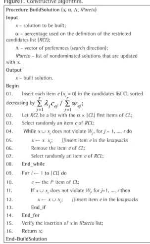
The candidates list CL is defined in line 1, which is formed by all the items out of the knapsacks. The CL list is sorted in decreasing order according to the ratio (1). As showed in line 3, the restricted candidates list (RCL) is composed by the α × |CL| first items of CL list. The loop in lines 4-8 is responsible by the randomization of the algorithm. An item e is randomly selected from RCL and inserted in x. This process is repeated while the insertion of e does not violate the capacity of the knapsacks. The loop in lines 9-14 looks for additional insertions from CL. This stage is greedy, respecting the sorting of CL list, and try to improve, if possible, the solution found in the previous stage (loop in lines 4-8). Experiments have shown that only very few items are inserted during this stage. Thus, an improvement in the current solution
3.1.
Greedy randomized construction
To generate an initial set of dominating solutions, a greedy heuristic is used to maximize a linear combination of the objective functions:
1
r j j
j= f ( x )
λ ∑ where 1 1 r j j= λ =
∑ and 0 ≤λj≤ 1, ∀j.
The preference vector Λi = (λ1, …, λr) determinates the search direction i on the Pareto optimal frontier. For building a solution, first, a preference vector Λi
is defined. For this vector is generated a solution x, whose weighted function f(x) is maximized.
Murata et al. (2001) introduces a way of generating the preference vector distributed uniformly on the Pareto frontier. Each component of the vector Λ = (Λ1,
Λ2, …, Λm) is generated combining r non-negatives integers with sum equal to s,
v1 + v2 + … + vr = s, where vi∈ {0, ..., s},
which is a value large enough to produce m search directions. The number of generated search directions for r objectives and a value s, Nr(s), is calculated as follows:
N2(s) = s + 1.
N3(s) = 2
0 0 1 1 2 2
s s
i= N ( i ) =i= ( i ) ( s )( s ) /
+ = + +
∑ ∑ .
N4(s) = 3
0 0 1 2 2
s s
i= N ( i ) i− ( i )( i ) /
= + +
∑ ∑ .
For instance, for r = 2 objectives and s = 5 we have 6 vectors (v1, v2): (0,5), (1,4), (2,3), (3,2), (4,1) and (5,0). For r = 3 and s = 3 we have 10 vectors (v1, v2, v3): (0,0,3), (0,1,2), (0,2,1), (0,3,0), (1,0,2), (1,1,1), (1,2,0), (2,0,1), (2,1,0) and (3,0,0).
With the goal of obtaining normalized directions ( 1 1 r j j= λ =
∑ ) we calculate λj = vj/s, vj∈ {0, 1, 2, ..., s}. Figure 1 presents the implemented constructive algorithm, BuildSolution, which is a greedy randomized algorithm that builds a solution by inserting items with the higher value for the following ratio:
1 1 r j ej j r ej j c w = = λ ∑ ∑ (1)
Figure1. Constructive algorithm. ProcedureBuildSolution (x, α, Λ, lPareto) Input
x – solution to be built;
α – percentage used on the definition of the restricted candidates list (RCL);
Λ – vector of preferences (search direction);
lPareto – list of nondominated solutions that are updated with x.
Output
x – built solution. Begin
01. Insert each item e (xe = 0) in the candidates list CL sorted
decreasing by
= =
∑λ ∑
1 1
/ ;
r r
j ej ej j c j w
02. Let RCL be a list with the α × |CL| first items of CL; 03. Select randomly an item e of RCL;
04. While x ∪ xe does not violate Wj , for j = 1, ..., r do
05. x ¬ x xe; //insert item e in the knapsacks
06. Remove the item e of CL; 07. Select randomly an item e of RCL; 08. End_while
09. For i ¬ 1 to |CL| do 10. e ¬ the ith item of CL;
11. If x ∪ xe does not violate Wj, for j=1, ..., r then
12. x ¬ x ∪ xe; //insert item e in the knapsacks
13. End_if 14. End_for
15. Verify the insertion of x in lPareto list; 16. Return x;
is out of the knapsack that cannot be inserted without violating any restriction of the problem. In other words, the items are removed from the knapsacks until the free space obtained in this way allows the insertion of any item that remains out of the knapsacks. This step is completely greedy. In line 6, the BuildSolution
algorithm is executed completing the construction of the solution y.
If the new solution, y, is better than x, then the solution x is updated at line 8 and the vector Marked is reinitialized in lines 9-10. Otherwise, in line 13, the first element that was removed from y during the stage described in line 5 is marked. In line 16, the refined solution, x, is returned.
The number of iterations of the local search algorithm depends on the quality of the initial solution x received as a parameter.
3.3.
MGRASP algorithm
Figure 3 presents the proposed MGRASP algorithm, which receives as input parameters the number of iterations (N_iter), the percentage α used at the construction phase and the percentage β used at the local search phase. Parameters α and β were empirically set at 10% and 50%, respectively. As output, the algorithm returns the lPareto list, where the nondominated solutions are stored. In line 1, the lPareto list is initialized. The loop in lines 2-7 executes N_iter GRASP iterations. In line 3, the solution x is initialized. The search direction Λi is defined in line 4. The solution x is built by the BuildSolution
procedure in line 5. In line 6, the solution x is refined. Finally, the lPareto list is returned.
can be achieved without compromising the greedy-randomized feature of the algorithm. In line 15 it is verified if solution x is a nondominated solution and, finally, the solution x is returned in line 16.
3.2.
Local search
Figure 2 presents the LocalSearch algorithm that removes the worst items from the knapsacks according to the ratio (1) and uses the BuildSolution algorithm
to produce a new solution. This algorithm receives as input parameters the solution x to be refined, the percentage β that is used at the solution reconstruction stage, the search direction Λ and the lPareto list,
where the nondominated solutions are stored. The loop in lines 1-2 initializes all the positions of the vector Marked with false. An item e can be
removed from the knapsack only if Marked[e] = false.
The loop in lines 3-15 is executed while exist elements that can be removed, that is, elements still unmarked. In line 4, the solution x is assigned to the auxiliary solution y. In line 5, the element that present the shortest value of the ratio (1) is removed from y. This process is repeated while there exists an element that
Figure 2. Local search algorithm. ProcedureLocalSearch (x, β, Λ, lPareto) Input
x – solution to be refined;
β – percentage used at the reconstruction of solution x; Λ – vector of preferences (search direction);
lPareto – list of nondominated solutions. Output
x – refined solution. Begin
01. For i ¬ 1 to n do 02. Marked[i] ¬false;
03. While there exists an item e such that Marked[e] = false do 04. y ¬ x;
05. Remove the unmarked item j (yj = 1) that presents the
smallest value of the ratio (1). Repeat this process until any item g (yg = 0) may be chosen for insertion;
06. y ¬BuildSolution (y, β, Λ, lPareto); 07. If f(y) > f(x) then
08. x ¬ y; 09. For i ¬ 1 to n do 10. Marked[i] ¬false; 11. Else
12. Let xe be the unmarked item of x that presents the
smallest value of the ratio 1; 13. Marked[e] ¬true; 14. End_if
15. End_while 16. Return x; End-LocalSearch
Figure 3. MGRASP algorithm. ProcedureMGRASP (N_iter, α, β) Input
N_iter – number of GRASP iterations; α – percentage used at the construction stage; β – percentage used at the local search stage. Output
lPareto – list of nondominated solutions. Begin
01. lPareto ¬∅; 02. For i ¬ 1 to N_iter do 03. x ¬∅;
04. Let Λi be the search direction in the position i of Λ,
defined according to the preference specification method described at Subsection 3.1;
05. x ¬BuildSolution (x, α, Λi, lPareto);
06. x ¬LocalSearch (x, β, Λi, lPareto);
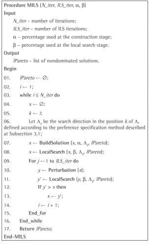
returns the lPareto list, where the nondominated solutions are stored. In line 1, the lPareto list is initialized. The loop in lines 3-16 executes N_iter iterations. In line 4, the solution x is initialized. The search direction Λk is defined in line 6. The solution x is built in line 7 and refined in line 8. The loop in lines 9-15 executes ILS_iter ILS iterations. In line 10, the perturbation method is applied at solution x. The resulting solution y is refined in line 11. If the refined solution is better than x, x is updated in line 13. Finally, the lPareto list is returned.
5. Computational experiments
We compare the results of MGRASP and MILS
algorithms with the following genetic algorithms:
MOTGA (ALVES; ALMEIDA, 2007), MOGLS
(JASKIEWICZ, 2002) and SPEAII (ZITZLER; LAUMANNS; THIELE, 2002).
All computational experiments with the MGRASP
and MILS algorithms were performed on a 3.2GHz Pentium IV processor with 1 Gbyte of RAM memory. Both algorithms were implemented in C using version 6.0 of the Microsoft Visual C++ compiler.
4. Multiobjective ILS algorithm – MILS
The Iterated Local Search (ILS) algorithm (LOURENÇO; MARTIN; STÜTZLE, 2002) involves the repeated application of a local search algorithm applied to the candidate solutions found by a broader search process that involves a biased random walk through the search space.
The algorithm works by first building an initial solution, which is refined using a local search strategy. The algorithm loop involves three steps: a perturbation of the current solution, the application of the local search to the perturbed solution, and an acceptance decision of whether or not the locally optimizing candidate solution should replace the current working solution for the search.
Subsection 4.1 presents the perturbation method used in the proposed multiobjective ILS algorithm (MILS algorithm). The description of the MILS
algorithm is given in Subsection 4.2.
4.1.
Perturbation
In the proposed perturbation method, we exchange the content of two regions of a solution x. The size of the regions is chosen randomly between the interval [1, γ × n], where n is the number of items and γ was empirically set at 10%. Figure 4 shows an example of perturbation, in which the content of regions 1 and 2 are exchanged. After applying the perturbation method, the solution x can be infeasible. If it happens, we randomly select an item to be removed from the knapsack. This process is repeated until x becomes feasible.
4.2.
MILS algorithm
Figure 5 presents the proposed MILS algorithm,
which receives as input parameters the number of iterations (N_iter), the number of ILS iterations (ILS_ iter), the percentage α used at the construction phase and the percentage β used at the local search phase.
Parameters ILS_iter, α and β were empirically set at 5, 0% and 10%, respectively. As output, the algorithm
Figure 4. Example of perturbation.
Figure 5. MILS algorithm. ProcedureMILS (N_iter, ILS_iter, α, β) Input
N_iter – number of iterations; ILS_iter – number of ILS iterations; α – percentage used at the construction stage; β – percentage used at the local search stage. Output
lPareto – list of nondominated solutions. Begin
01. lPareto ¬∅; 02. i ¬ 1;
03. while i ≤ N_iter do 04. x ¬∅; 05. k ¬ i;
06. Let Λk be the search direction in the position k of Λ,
defined according to the preference specification method described at Subsection 3.1;
07. x ¬BuildSolution (x, α, Λk, lPareto);
08. x ¬LocalSearch (x, β, Λk, lPareto);
09. For j ¬1 to ILS_iter do 10. y ¬Perturbation (x);
11. y’ ¬LocalSearch (y, β, Λk, lPareto);
Note that Davg is the average distance from a point z ∈ R to its closest point in H.
When the Pareto optimal set is not known and H’ is the set of nondominated points generated by another heuristic method, we define the reference set R as the nondominated points of (H ∪ H’) and use the same measures mentioned above to assess the approximation of H and H’ relative to R.
We also use an additional measure to compare two nondominated solutions sets, H and H’. This measure is called strict coverage (ALVES; ALMEIDA, 2007; JASKIEWICZ, 2002; ZITZLER; THIELE, 1999) and computes the fraction of solutions of one set dominated by solutions of another set. The strict coverage measure is defined as
(
)
{
z' H' z H : z dominates z'}
C H ,H'H' ∈ ∃ ∈ =
The value C(H, H’) = 1 means that all points of H’ are dominated by points of H. The value C(H, H’) = 0 means that no point of H’ is dominated by any point of H.
5.3.
Results comparison
The experiments done were conducted using the test instances described in Table 1, which were proposed by Zitzler and Thiele (1999), and has been also used by MOTGA (ALVES; ALMEIDA, 2007),
MOGLS (JASKIEWICZ, 2002) and SPEAII (ZITZLER;
LAUMANNS; THIELE, 2002) algorithms.
In the first experiment, the MGRASP algorithm
was run five times to each instance. Each run finished when the average running time spent by MOTGA
algorithm (the fastest algorithm among MOTGA,
MOGLS and SPEAII) was achieved. The goal of this
experiment is to evaluate MGRASP, MOTGA, MOGLS
and SPEAII algorithms running the same time in a
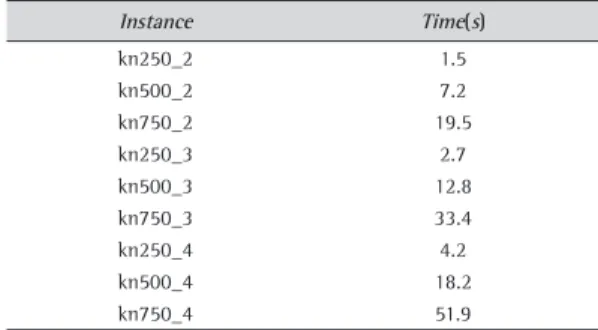
similar machine. Table 2 shows the average running times of MOTGA. In this experiment, we use the
5.1.
Test instances
In this work, we use the set of instances proposed by Zitzler and Thiele (1999). They generated instances with 250, 500 and 750 items, and 2, 3, and 4 objectives. Uncorrelated profits and weights were randomly generated in the interval [10, 100]. The knapsack capacities were set to half the total weight regarding the corresponding knapsack:
Wj = 0.5
1 n
ij i=w .
∑
The problem instances are presented in Table 1 and are available at: http://www.tik.ee.ethz.ch/~zitzler/ testdata.html.
5.2.
Evaluation of computational results in
multiobjective optimization
The quality of a solution of a single-objective minimization problem is evaluated in a straightforward manner as the relative difference between the objective value of such solution and the value of an optimal solution. In multiobjective optimization, however, there is no natural single measure that is able to capture the quality of a nondominated set H to the Pareto optimal set or reference set R.
We measure the quality of the nondominated set H generated by the heuristic method relative to the reference set R by using two measures:
• Cardinal measure: number of reference solutions, NRS, found by the heuristic method, where NRS = |H∩R|; and
• Average distance measure (proposed by Czyzak and Jaszkiewicz (1998) and Ulungu, Teghen and Ost (1998)): average distance between the nondominated set H generated by the heuristic method and the reference set R. We measure the average distance Davg with
1
avg z' H
z R
D min d ( z', z ),
R ∈
∈
= ∑ where
d is defined byd ( z', z ) =maxj=1,...,r( z'j−z ),j z’ = (z’1, …, z’r) ∈ H and z = (z1, …, zr) ∈ R.
Table 1. Test instances.
Instance Objectives Items
kn250_2 2 250
kn250_3 3 250
kn250_4 4 250
kn500_2 2 500
kn500_3 3 500
kn500_4 4 500
kn750_2 2 750
kn750_3 3 750
kn750_4 4 750
Table 2. Average running times of MOTGA algorithm on a Pentium IV 3.2 GHz.
Instance Time(s)
kn250_2 1.5
kn500_2 7.2
kn750_2 19.5
kn250_3 2.7
kn500_3 12.8
kn750_3 33.4
kn250_4 4.2
kn500_4 18.2
instance, the number of reference solutions (NRS) and the average distance (Davg). The best results are highlighted in bold.
The results show that when the number of reference solutions (NRS) is compared, the MILS
algorithm generates a larger number of reference solutions for all instances. So, by the cardinal measure,
MILS performs better than the others algorithms. When the average distance, Davg, is compared, MILS
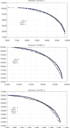
also performs better than the others algorithms. Figure 7 shows the solutions obtained by MILS,
MOTGA, MOGLS and SPEAII algorithms after a
running of the test instances “kn250_2”, “kn500_2” and “kn750_2”. In this figure, we also can see that the solution set obtained by MILS is better distributed.
In the third experiment, MGRASP and MILS
algorithms are compared using the strict coverage measure presented in Subsection 5.2. The results are presented in Figure 8. When the instances with 2 objectives are analyzed, we can see that the majority of the solutions obtained by MGRASP are dominated
by the solutions obtained by MILS. When the instances
with 3 and 4 objectives are compared, we can see that just a few of the solutions obtained by both algorithms are dominated by the solutions obtained by the other algorithm.
For making a better comparison between MGRASP
and MILS algorithms, a fourth experiment was done.
In this experiment, both algorithms were run five times cardinal measure (NRS) and the average distance
measure (Davg) presented in Subsection 5.2.
Table 3 presents comparative results for the first experiment. In the second column we have the number |R| of reference solutions. In the following columns are presented, for each algorithm (MGRASP, MOTGA,
MOGLS and SPEAII) and for each instance, the number
of reference solutions (NRS) and the average distance (Davg). The best results are highlighted in bold.
The results show that when the number of reference solutions (NRS) is compared, the MGRASP
algorithm generates a larger number of reference solutions on 7 instances from a total of 9 instances. So, by the cardinal measure, MGRASP performs
better than the others algorithms. When the average distance, Davg, is compared, MGRASP also performs better than the others algorithms.
Figure 6shows the solutions obtained by MGRASP,
MOTGA, MOGLS and SPEAII algorithms after a
running of the test instances “kn250_2”, “kn500_2” and “kn750_2”. In this figure, we can see that the solution set obtained by MGRASP is better distributed.
In the second experiment, the previous experiment is repeated with MILS, MOTGA, MOGLS and SPEAII
algorithms. Table 4 presents comparative results for the second experiment. In the second column we have the number |R| of reference solutions. In the following columns are presented, for each algorithm
(MILS, MOTGA, MOGLS and SPEAII) and for each
Table 3. Comparison of MGRASP, MOTGA, MOGLS and SPEAII algorithms running the same time in a similar machine.
Instance |R| NRS Davg
MGRASP MOTGA MOGLS SPEAII MGRASP MOTGA MOGLS SPEAII
kn250_2 162.0 86.4 73.0 3.4 - 0.0016 0.0025 0.0094 -Kn500_2 227.0 68.8 166.4 0.2 - 0.0030 0.0009 0.0181 -Kn750_2 313.0 75.2 236.6 1.2 0.0 0.0036 0.0007 0.0190 0.0550 Kn250_3 3379.0 1701.4 456.0 1221.6 - 0.0016 0.0118 0.0128 -Kn500_3 6517.4 3709.4 981.6 1826.4 - 0.0013 0.0101 0.0210 -Kn750_3 8692.6 4851.0 1378.0 2258.8 204.8 0.0014 0.0091 0.0220 0.0887 Kn250_4 9125.2 4358.0 1002.4 3764.8 - 0.0059 0.0226 0.0182 -Kn500_4 14809.8 7418.4 2054.6 5336.8 - 0.0068 0.0212 0.0270 -Kn750_4 19458.8 9700.8 2982.6 6515.6 259.8 0.0071 0.0193 0.0307 0.1504
Table 4. Comparison of MILS, MOTGA, MOGLS and SPEAII algorithms running the same time in a similar machine.
Instance |R| NRS Davg
MILS MOTGA MOGLS SPEAII MILS MOTGA MOGLS SPEAII
The results show that when the number of reference solutions (NRS) is compared, the MILS
algorithm generates a larger number of reference solutions on 8 instances from a total of 9 instances. When the average distance, Davg, is compared, the
MILS algorithm has a smaller average distance on 8
instances from a total of 9 instances. When the time consumed is compared, similar results are obtained by both algorithms.
Figure 7. Solution obtained by MILS, MOTGA, MOGLS and
SPEAII.
to each instance. Each run finished after N_iter = 1000 iterations. Table 5 presents comparative results for the fourth experiment. In the second column we have the number |R| of reference solutions. In the following columns are presented, for each algorithm (MGRASP
and MILS) and for each instance, the number of
reference solutions (NRS), the average distance (Davg) and the time consumed in seconds. The best results are highlighted in bold.
Figure 6. Solution obtained by MGRASP, MOTGA, MOGLS
and SPEAII.
Table 5. Comparison of MILS and MGRASP.
Instance |R| NRS Davg Time (s)
MILS MGRASP MILS MGRASP MILS MGRASP
Kn250_2 305.6 281.6 36.4 0.0001 0.0027 12.2 10.9
Kn500_2 549.2 540.8 8.8 0.0001 0.0032 70.8 62.8
Kn750_2 764.4 735.4 29.2 0.0001 0.0023 217.1 189.3
compared, the MGRASP algorithm obtained a smaller average distance on 7 instances from a total of 9 instances. The MILS algorithm obtained a smaller
average distance for all instances. It was also noted that the solutions sets obtained by MGRASP and
MILS algorithms are better distributed than the ones obtained by the others algorithms.
When the proposed algorithms are compared, it is concluded that the MILS performs better than
MGRASP. When the number of reference solution
(NRS) is compared, the MILS algorithm generates a larger number of reference solutions on 8 instances from a total of 9 instances. When the average distance (Davg) is compared, the MILS algorithm obtained a
smaller average distance on 8 instances from a total of 9 instances. Similar times consumed are obtained by both algorithms.
Based on the obtained results, it is concluded that the proposed algorithms, MGRASP and MILS,
are very robust, outperforming three efficient genetic
6. Conclusion
In this paper, we have proposed local search based algorithms, MGRASP and MILS, to generate a
good approximation of the set of efficient or Pareto optimal solutions of a multiobjective combinatorial optimization problem. They are applied for solving the knapsack problem with r objectives and they are compared with MOTGA algorithm, proposed by Alves
and Almeida (2007), MOGLS algorithm, proposed by Jaskiewicz (2002), and SPEAII algorithm, proposed
by Zitzler, Laumanns and Thiele (2002).
In the experiments comparing the proposed algorithms with MOTGA, MOGLS and SPEAII
algorithms, when the number of reference solution (NRS) is compared, the MGRASP algorithm generates a larger number of reference solutions on 7 instances from a total of 9 instances. The MILS algorithm generates a larger number of reference solutions for all instances. When the average distance (Davg) is
via genetic algorithms and discrete event simulation. Pesquisa Operacional, v. 29, n. 1, p. 43-66, 2009. http:// dx.doi.org/10.1590/S0101-74382009000100003 LOURENÇO, H. R.; MARTIN, O. C.; STÜTZLE, T. Iterated
local search. In: GLOVER, F.; KOCHENBERGER, G. (Eds.). Handbook of Metaheuristics. Kluwer, 2002. p. 321-353. MAURI, G. R.; LORENA, L. A. N. Uma nova abordagem
para o problema dial-a-ride. Produção, v. 19, n. 1, p. 41-54, 2009. http://dx.doi.org/10.1590/S0103-65132009000100004
MURATA, T.; ISHIBUCHI, H.; GEN, M. Specification of genetic Search directions in cellular multi-objective genetic algorithms. In: INTERNATIONAL CONFERENCE ON EVOLUTIONARY MULTI-CRITERION OPTIMIZATION, 2001, Zurich. Proceedings... Zurich: Springer, 2001. v. 1, p. 82-95.
RESENDE, M. G. C.; RIBEIRO, C. C. Greedy randomized adaptive search procedures. In: GLOVER, F.; KOCHENBERGER, G. (Eds.). Handbook of Metaheuristics. Boston: Kluwer, 2003. p. 219-249.
RIBEIRO, C. C. et al. A hybrid heuristic for a multi-objective real-life car sequencing problem with painting and assembly line constraints. European Journal of Operational Research, v. 191, p. 981-992, 2008. http:// dx.doi.org/10.1016/j.ejor.2007.04.034
ULUNGU, E. L.; TEGHEM, J. The two phases method: An efficient procedure to solve bi-objective combinatorial optimization problems. Foundations of Computing and Decision Sciences, v. 20, n. 2, p. 149-165, 1995. ULUNGU, E. L.; TEGHEM, J.; OST, C. Efficiency of interactive
multi-objective simulated annealing through a case study. Journal of the Operational Research Society, v. 49, p. 1044-1050, 1998.
VAN VELDHUIZEN D. A.; LAMONT, G. B. Multiobjective evolutionary algorithms: Analyzing the state-of art. Evolutionary Computation, v. 8, n. 2, p. 125-147, 2000. http://dx.doi.org/10.1162/106365600568158
VIANNA, D. S. et al. Parallel strategies for a multi-criteria GRASP algorithm. Produção, v. 17, p. 1-12, 2007. http:// dx.doi.org/10.1590/S0103-65132007000100006 VISÉE, M. et al. Two-Phases Method and Branch and Bound
Procedures to solve the Bi-objectives knapsack Problem. Journal of Global Optimization, v. 12, p. 139-155, 1998. http://dx.doi.org/10.1023/A:1008258310679
ZITZLER, E.; THIELE, L. Multiobjective evolutionary algorithms: A comparative case study and the strength pareto approach. IEEE Transactions on Evolutionary Computation, v. 3, n. 4, p. 257–271, 1999. http://dx.doi. org/10.1109/4235.797969
ZITZLER, E.; LAUMANNS, M.; THIELE, L. SPEA2: Improving the Strength Pareto Evolutionary Algorithm. In: GIANNAKOGLOU, K. et al. (Eds.). Evolutionary Methods for Design, Optimization and Control with Applications to Industrial Problems. Athens, 2002. p. 95-100.
Acknowledgements
This work was finantiated by: Conselho Nacional de Desenvolvimento Científico e Tecnológico (CNPq); Fundação de Amparo à Pesquisa do Estado do Rio de Janeiro (FAPERJ); Parque de Alta Tecnologia do Norte Fluminense (TECNORTE); and Fundação Estadual do Norte Fluminense (FENORTE).
algorithms from the literature: MOTGA, MOGLS and
SPEAII. We can also conclude that the MILS algorithms
performs better than the MGRASP algorithm.
New researches will be done to incorporate memory mechanisms in the MILS and MGRASP algorithms,
trying to achieve better results using in each iteration, information obtained in previous iterations.
References
ALVES, M. J.; ALMEIDA, M. M. A multiobjective Tchebycheff based genetic algorithm for the multidimensional knapsack problem. Computers & Operations Research, v. 34, p. 3458-3470, 2007. http://dx.doi.org/10.1016/j. cor.2006.02.008
ARROYO, J. E. C.; VIEIRA, P. S.; VIANNA, D. S. A GRASP algorithm for the multi-criteria minimum spanning tree problem. Annals of Operations Research, v. 159, p. 125-133, 2008. http://dx.doi.org/10.1007/s10479-007-0263-4
COELLO, C. A. C. An updated survey of GA-based multiobjective optimization techniques. ACM Computing Surveys, v. 32, n. 2, p. 109-143, 2000. http://dx.doi. org/10.1145/358923.358929
CZYZAK, P.; JASZKIEWICZ, A. Pareto simulated annealing – a metaheuristic technique for multiple objective combinatorial optimization. Journal of Multi-Criteria Decision Analysis, v. 7, p. 34-47, 1998. http://dx.doi. org/10.1002/(SICI)1099-1360(199801)7:1<34::AID-MCDA161>3.0.CO;2-6
DEB, K. Multi-objective optimization using evolutionary algorithms. England: John Wiley & Sons Ltd., 2004. EHRGOTT, M.; GANDIBLEUX, X. A survey and annotated
bibliography of multiobjective combinatorial optimization. OR Spektrum, v. 22, p. 425-460, 2000. http://dx.doi.org/10.1007/s002910000046
EPPRECHT, E. K.; LEIRAS, A. Otimização conjunta de gráficos de X-barra-S ou X-barra-R: um procedimento de fácil implementação. Produção, v. 17, n. 3, p. 520-535, 2007. FEO, T. A.; RESENDE, M. G. C. Greedy randomized adaptive
search procedures. Journal of Global Optimization, v. 6, p. 109-133, 1995. http://dx.doi.org/10.1007/ BF01096763
GANDIBLEUX, X.; FRÉVILLE, A. Tabu search based procedure for solving the 0-1 multiobjective knapsack problem: The two objectives case. Journal of Heuristics, v. 6, p. 361-383, 2000. http://dx.doi. org/10.1023/A:1009682532542
HANSEN, P. Tabu search for multiobjective optimization: MOTS. Technical Report. Technical University of Denmark. In: INTERNATIONAL CONFERENCE ON MULTIPLE CRITERIA DECISION MAKING, 13., 1997, Cape Town. Proceedings... Cape Town, 1997.
JASKIEWICZ, A. On the performance of multiple objective genetic local search on the 0/1 knapsack problem: A comparative experiment. IEEE Transaction on Evolutionary Computation, v. 6, n. 4, p. 402-412, 2002. http://dx.doi.org/10.1109/TEVC.2002.802873
JONES, D. F.; MIRRAZAVI, S. K.; TAMIZ, M. Multi-objective metaheuristics: An overview of the current state-of-art. European Journal of Operational Research, v. 137, p. 1-19, 2002. http://dx.doi.org/10.1016/S0377-2217(01)00123-0