Gonçalo Filipe Torcato Mordido
Master of ScienceAutomated Organisation and Quality Analysis of
User-Generated Audio Content
Dissertation submitted in partial fulfillment of the requirements for the degree of
Master of Science in
Computer Science and Engineering
Adviser: Prof. Dr. Sofia Cavaco, Assistant Professor, Faculdade de Ciências e Tecnologia da Universidade Nova de Lisboa
Co-adviser: Prof. Dr. João Magalhães, Assistant Professor, Facul-dade de Ciências e Tecnologia da UniversiFacul-dade Nova de Lisboa
Examination Committee
Chairperson: Prof. Dr. Fernando Birra Raporteurs: Prof. Dr. Fernando Perdigão
Automated Organisation and Quality Analysis of User-Generated Audio Con-tent
Copyright © Gonçalo Filipe Torcato Mordido, Faculty of Sciences and Technology, NOVA University of Lisbon.
The Faculty of Sciences and Technology and the NOVA University of Lisbon have the right, perpetual and without geographical boundaries, to file and publish this dissertation through printed copies reproduced on paper or on digital form, or by any other means known or that may be invented, and to disseminate through scientific repositories and admit its copying and distribution for non-commercial, educational or research purposes, as long as credit is given to the author and editor.
A c k n o w l e d g e m e n t s
This work was partially funded by the H2020 ICT project COGNITUS with the grant agreement No 687605 and by the project NOVA LINCS Ref. UID/CEC/04516/2013 in the form of a research grant which I am very grateful for. I would like to firstly thank Prof. Dr. Sofia Cavaco for all the tireless help and knowledge given during this last year, together with an exceptional work ethic. I could have not asked for a better supervisor. I would also like to thank Prof. Dr. João Magalhães for pointing me towards the right directions work-wise, and for all the life advice and insights that will certainly be remembered throughout my life.
A b s t r a c t
The abundance and ubiquity of user-generated content has opened horizons when it comes to the organization and analysis of vast and heterogeneous data, especially with the increase of quality of the recording devices witnessed nowadays. Most of the activity experienced in social networks today contains audio excerpts, either by belonging to a certain video file or an actual audio clip, therefore the analysis of the audio features present in such content is of extreme importance in order to better understand it. Such understanding would lead to a better handling of ubiquity data and would ultimately provide a better experience to the end-user.
The work discussed in this thesis revolves around using audio features to organize and retrieve meaningful insights from user-generated content crawled from social me-dia websites, more particularly data related to concert clips. From its redundancy and abundance (i.e., for the existence of several recordings of a given event), recordings from musical shows represent a very good use case to derive useful and practical conclusions around the scope of this thesis.
Mechanisms that provide a better understanding of such content are presented and al-ready partly implemented, such as audio clustering based on the existence of overlapping audio segments between different audio clips, audio segmentation that synchronizes and
relates the different cluster’s clips in time, and techniques to infer audio quality of such
clips. All the proposed methods use information retrieved from an audio fingerprinting algorithm, used for the synchronization of the different audio files, with methods for
filtering possible false positives of the algorithm being also presented.
For the evaluation and validation of the proposed methods, we used one dataset made of several audio recordings regarding different concert clips manually crawled
from YouTube.
R e s u m o
A abundância e ubiquidade de conteúdo gerado por utilizadores tem aberto novos horizontes na organização e análise de grandes quantidades de dados heterogéneos, es-pecialmente com o aumento da qualidade dos dispositivos de gravação observada hoje em dia. A maior parte da atividade experienciada nas redes sociais hoje contém excertos de áudio, quer provenientes de ficheiros de vídeo, quer de clips áudio. Assim, a análise das características do áudio presente nesse conteúdo é de extrema importância para o seu melhor entendimento. Tal compreensão levaria a uma melhor manipulação de dados ubíquos e providenciaria uma melhor experiência de utilização para o consumidor final. O trabalho discutido nesta tese consiste em usar características de áudio para organi-zar e derivar perceções significativas de conteúdo gerado por utilizadores tirado de redes sociais, mais especificamente dados relativos a concertos musicais. Tendo em conta a sua redundância e abundância (i.e., por haver várias gravações relativas a um dado evento), gravações de concertos representam um bom caso de uso para derivar conclusões úteis, num contexto prático, no âmbito desta tese.
Mecanismos que providenciam um melhor conhecimento de tal conteúdo são apresen-tados, como, por exemplo, o agrupamento baseado em segmentos sobrepostos entre clips diferentes de áudio, segmentação do áudio baseado em como esses clips se relacionam em termos de tempo, e técnicas para inferir a qualidade das amostras. Todos os métodos propostos usam informação retornada por um algoritmo deaudio fingerprinting, usado para a sincronização dos diferentes ficheiros, com métodos de filtragem de possíveis falsos positivos por parte do algoritmo sendo também apresentados.
Os diferentes métodos propostos pela nossa solução foram testados e validados usando um conjunto de dados construído a partir de gravações de áudio de diferentes músicas de concertos, retirados manualmente do YouTube.
C o n t e n t s
List of Figures xiii
List of Tables xvii
Listings xix
1 Introduction 1
1.1 Objectives . . . 1
1.2 COGNITUS project . . . 3
1.3 Proposed solution . . . 4
1.4 Document outline . . . 7
2 Fundamental concepts 9 2.1 The basics of sound . . . 9
2.1.1 Sinusoids . . . 9
2.1.2 Sound wave properties . . . 10
2.1.3 Fast Fourier Transform . . . 12
2.1.4 Spectrogram . . . 13
2.2 Classification techniques . . . 14
2.2.1 Cross-Validation . . . 15
2.2.2 Logistic Regression . . . 15
2.2.3 K-Nearest Neighbours . . . 17
2.2.4 Support Vector Machines. . . 18
2.3 Hierarchical Clustering . . . 21
3 State-of-the-art 23 3.1 Audio fingerprinting . . . 23
3.1.1 Features extraction . . . 24
3.1.2 Fingerprint generation . . . 25
3.1.3 Robust audio hashing . . . 26
3.1.4 Searching process . . . 27
3.1.5 Matching process . . . 28
3.1.7 Possible applications . . . 30
3.2 Audio Clustering . . . 31
3.2.1 Graph structure using fingerprinting . . . 32
3.2.2 Interest inference . . . 32
3.2.3 Higher quality audio selection . . . 32
4 Proposed solution 35 4.1 Proposal . . . 35
4.2 Audio synchronisation . . . 37
4.3 Audio clustering . . . 37
4.4 Quality inference . . . 40
4.5 Audio segmentation . . . 41
4.5.1 Time-based segmentation . . . 42
4.5.2 Segmented quality inference . . . 43
4.6 Matches filtering. . . 45
4.6.1 Derivatives approach . . . 46
4.6.2 Learning approach . . . 49
4.7 Component integration . . . 54
5 Evaluation and results 57 5.1 Test setup. . . 57
5.2 Audio clustering . . . 59
5.3 Matches filtering - Derivatives approach . . . 64
5.4 Audio segmentation . . . 66
5.5 Audio quality inference . . . 67
5.6 Matches filtering - Learning approach . . . 68
5.6.1 Training set . . . 69
5.6.2 Parameters setting . . . 69
5.6.3 Prediction results . . . 70
6 Conclusion 75 6.1 Future work . . . 77
Bibliography 79
A Accepted scientific papers 83
L i s t o f F i g u r e s
1.1 Smartphone video capture in a music act. Source: [8] . . . 2
1.2 User-generated Content creation. Source: [8] . . . 2
1.3 Overview of the main project steps, concerning the FCT/UNL work plan. . . 4
1.4 Grouping of different audio files. Source: [44]. . . . . 5
1.5 Time-aligned audio files. Information about the quality of each file is very useful to choose which one of the audio clips should be played. Source: [9].. . . 5
1.6 Diagram of the different methods needed to achieve the organisation, segmentation, and quality analysis of a large dataset of audio files. . . 6
2.1 Sinusoid relation between displacement and time. Source: [3] . . . 10
2.2 Amplitude representation on a waveform. Source: [28] . . . 10
2.3 Frequency variations on a waveform. Source: [28] . . . 11
2.4 Sinusoid split in sections of phase in degrees. Source: [41] . . . 12
2.5 Representation of a zero-phase sinusoid (in blue) and a 270º angle phased sinusoid (in pink). Source: [1] . . . 12
2.6 Spectrogram captured of a recording of some words. Source: [53]. . . 13
2.7 Example of two classification problems. The samples of each class are repre-sented with different colours. On the left, the problem is linearly separable since all samples of each class can be separated by a line. On the right, the problem is non-linearly separable and another approach had to be used to separate both classes (a circle with radius r). Source: [42] . . . 14
2.8 Example of a Logistic function. Source: [18] . . . 16
2.9 Comparison of using a different number of neighbours for the classifier (1, 13 and 25, respectively). Source: [23] . . . 17
2.10 Different runs of the Logistic Regression classifier result in different positions of the frontier that separates both classes. Source: [23] . . . 18
2.12 Different values ofcwere used for different runs of the SVM. For the left image ac
value of 1 was used, where it is visible several support vectors being placed inside the margins (outlined with red circles), whilst in the right imagecwas equal to 1000 and no margin violations are observed. Source: [23] . . . 20
2.13 Example of hierarchical clustering. Source: [52] . . . 21
2.14 Example of agglomerative clustering. Source: [51] . . . 22
3.1 A spectrogram (in the left) with the correspondent extracted features on the right. Source: [50] . . . 25
3.2 Description of the hash generation process inShazam. Source: [50] . . . 26
3.3 Scatter plot of the timestamps of the different matches. Source: [49]. . . . 28
3.4 Histogram of the offsets of all matches. The real offset between the two clips is around
40 seconds, indicated by the peak in the histogram. Source: [49] . . . 29
3.5 Spectrogram containing the landmarks of a query song. . . 30
3.6 Spectrograms of a query song an a reference song with the matching landmarks high-lighted. . . 30
3.7 Spectrograms of both a query song and a song present in the database. The matching landmarks are highlighted in green. . . 31
4.1 Diagram representing the relation between the proposed methods. . . 36
4.2 Graph representation of a database with 3 different samples, withsong1sample1.mp3
andsong1sample2.mp3representing recordings of the same song (with a time offset
of 67.9 seconds between them) andsong2sample1.mp3being an unmatched sample by the audio fingerprinting algorithm. . . 39
4.3 The number of matching landmarks obtained increases with thehashes/secused in the Audio Fingerprinting algorithm. . . 43
4.4 As we increase the number ofhashes/sec, the number of samples with no matches returned by the Audio Fingerprinting algorithm decreases. . . 44
4.5 Distribution of the number of non-zero matches according to the segment duration. With 20hashes/secall segments between 1-2 seconds and 5-6 seconds had no match, but some matches occurred when using 100hashes/sec. . . 44
4.6 Distribution of matching landmarks between the matching samples. The breaking point indicates the last sample to be accepted as a true match, being all the files with lower percentage of matching landmarks than that sample discarded (in this case the 8th sample). . . 48
4.7 The variation of the regularisation parametercis represented in a logarithmic scale in the x-axis to promote an easier visualisation. From the differentc values,c = 8
L i s t o f F i g u r e s
4.8 As the number of neighbours increases after a certain threshold, we also notice a slightly increase on both validation and training error, meaning that the model is less restrained by local conditions but is more susceptible to producing wrong predictions. The k value that achieved the lowest validation error (≈0.0315) is when k = 15, being this the number of neighbours considered when dealing with the 2-feature combination. . . 52
4.9 Each parameter combination presented in the x-axis was returned at least once as the best parameters from performing grid-search using leave-one-song-out cross-validation. All retrieved pairs are then compared in terms of their model’s validation error, with the combination (c= 0.125, γ = 8) presenting the lowest validation error (≈0.0279). . . 53
5.1 Distribution of the various clip lengths of our dataset. . . 58
5.2 Distribution of the various clip lengths on the extended dataset.. . . 59
5.3 Analysis of the percentage of matching landmarks of the different matches
informa-tion in the matching lists where a false positive match was present. The derivatives that are lower than the derivative threshold (set to -0.07) are represented as yellow di-amonds, whereas the effectively discarded samples are represented with red squares.
Important to notice that samples can only be discarded if their percentage of match-ing landmarks is lower than the average of all samples’ matchmatch-ing landmarks in the matching list (represented as the blue dotted line in the graphs). . . 66
5.4 In these two examples of the matching lists of two different songs, since no
deriva-tive lower than the threshold was found bellow the average percentage of matching landmarks of the matching list (represented as the blue dotted line) no sample was discarded even though the last samples of each graphs were false positive matches (i.e., 5’th and 4’th sample, for the left-side and the right-side graphic respectively). . 68
5.5 Model errors of the different classifiers using the number of matching landmarks of
the right offset (#ML) and the total number of matching landmarks in all offsets found
(total#ML) as features. The parameter values with lowest validation errors (va) for
each classifier are: LR (c = 8, log(c) = 2.079,va≈0.0316), KNN (k = 15,va≈0.0315),
SVM (c= 0.125, γ= 8,va≈0.0279). . . 70
5.6 Model errors of the different classifiers using the number of matching landmarks of
the right offset (#ML), the total number of matching landmarks in all offsets found
(total#ML), and the number of landmarks of the query song (query#ML) as features. The parameter values with lowest validation errors (va) for each classifier are: LR (c =
8, log(c) = 2.079,va≈0.0342), KNN (k = 3,va≈0.0347), SVM (c= 8, γ= 2,va≈0.0279). 71
5.7 Model errors of the different classifiers using the number of matching landmarks of
the right offset (#ML), the number of landmarks of the query song (query#ML) and
matched song (match#ML) as features. The parameter values with lowest validation errors (va) for each classifier are: LR (c = 1, log(c) = 0, va ≈0.1582), KNN (k = 3,
5.8 Model errors of the different classifiers using the number of matching landmarks of
the right offset (#ML), the total number of matching landmarks in all offsets found
(total#ML), the number of landmarks of the query song (query#ML) and matched song (match#ML) as features. The parameter values with lowest validation errors (va) for each classifier are: LR (c = 16384, log(c) = 9.704,va≈0.0269), KNN (k = 3,
va≈0.0.0380), SVM (c= 215, γ= 2−11,va≈0.0243). . . 73
5.9 Accuracy of the best models (i.e., with lowest validation error) of each classifier for the different combination of features, with the respective parameter values described
inside each bar. The numbers placed on top of each bar represent the number of false positives retrieved by each model. . . 74
5.10 Accuracy of the models with lowest validation error that did not retrieved any false positives. The missing models represent that all retrieved models classified at least one false positive, with no classifier being able to surpass this constraint when using the features combination (#ML, total#ML, query#L). New models with different
L i s t o f Ta b l e s
4.1 Query songs’ offsets. . . . . 38
4.2 Example of sample repetition in the matching list (song5sample5.mp3appears 3 times). . . 46
4.3 Example of a false positive sample (song2sample5.mp3) in the matching list. The number of matching landmarks of that sample (7) and percentage (0.5 %) are the lowest in all matches. . . 47
5.1 Extended dataset information. A different number of samples and recording lengths was crawled for each song. . . 58
5.2 Extended dataset information. . . 59
5.3 Clustering benchmarks. . . 65
5.4 Filtering benchmarks using the derivatives analysis approach.. . . 65
L i s t i n g s
4.1 Input file example with the paths of the sound files. . . 39
4.2 Output file example. Two clusters were formed, and 2 samples were con-sidered unmatched. Cluster are represented by incremental id’s (starting at 1), and the different files of each cluster are represented by their file paths. . . 39
4.3 Example of output file with the different segments of cluster 1. . . . . 44 5.1 Output clusters file without filtering. Clusters which correctly grouped
only recordings from the same song/event are underlined.. . . 60
5.2 Output clusters file. . . 62
C
h
a
p
t
e
r
1
I n t r o d u c t i o n
In this dissertation we propose mechanisms to achieve a better understanding of user-generated content by the analysis of their correspondent audio signals. The different
methods permit the grouping of the different audio files by events, with supplementary
information about how the different files synchronise with each other in terms of the
event’s timeline. Since these organisation methods use solely the information retrieved by an audio fingerprinting algorithm, we also propose two novel methods for filtering possible false positives from the algorithm. Furthermore, we propose one novel method to infer the audio quality of the different files relative to the rest of the files in their cluster,
achieving more promising results in our test setup than the current state-of-the-art.
In this first chapter, we briefly described the main objectives of this work (section 1.1), introduce the project that motivated this thesis’ goals (section1.2), give an overview of the proposed methods (section 1.3), and, finally, we summarise the overall document structure (section1.4)
1.1 Objectives
The abundance and ubiquity of user-generated content experienced in social networks nowadays (figures1.1and1.2), generated the need to organise and analyse such vast and heterogeneous content. Such properties are fuelled by the increasingly need of sharing events in social media, together with the technology advancements that made all of this high-quality sharing possible in the first place. In this work, we focus on the audio con-tent of several user and professional recordings of different concert songs from different
festivals. Concert recordings represent a good use case for testing and validating the different proposed methods in this thesis since there are several recordings reporting the
the different samples, which consecutively allows their grouping and quality inference
by the execution of the proposed methods in this thesis.
User-generated content often contains audio cues, either by belonging to a certain video file or audio clip, and therefore the analysis of the audio features might promote a better understanding of that content. Such understanding would then lead to a better handling of ubiquity data and would ultimately provide a better experience to the end-user, which in our use case could be seen in the availability of a full length recording of a given concert song composed by joining different smaller length existing recordings
together, or by only presenting the higher quality recording to the user at a given time.
Figure 1.1:Smartphone video capture in a music act. Source: [8]
Figure 1.2: User-generated Content creation. Source: [8]
The objective of this research work is to analyse audio data derived from content uploaded by end-users on social media platforms and derive insights of the investigated data, such as for example performing audio clustering based on the existence of over-lapped audio segments between different audio files, with each cluster representing an
1 . 2 . CO G N I T U S P R O J E C T
content that will be further implemented in COGNITUS [8], a European project that pro-vided the main background and motivation for this thesis’ work, which will be described in the next section.
1.2 COGNITUS project
The research of this thesis started from a research grant under the European Union’s Horizon 2020 funded project COGNITUS. This project involves eight European partners, both from the industry and academics, namely BBC R&D, Queen Mary University of London, FORTH, Forthnet, Arris, VITEC, and Faculdade de Ciências e Tecnologia da Universidade Nova de Lisboa, with each of the partners having both individual and collaborative tasks.
The main aim of the project is to provide ultra-high definition (UHD) broadcasting generated from user-generated content, given its abundance in the social networks activi-ties. This quantity and ubiquity of information allied with the high-quality of recording now possible with the current state of the broadcasting devices (e.g., smart phones, tablets) served as basis for the project’s objectives. Therefore, the end goal of COGNITUS is to de-liver the proof of concept of a solution that supports high-quality and enables the upload of user-generated content, while promoting the enrichment of the end user’s broadcasting experience in form of an application.
In this vast and collaborative process, FCT/UNL efforts are spread across several
intimately related topics such as video annotation and analysis, event summarization, data quality inference, and collaborative audio composition. In order to integrate all these processes, an abstract view over the different assignments shall be made.
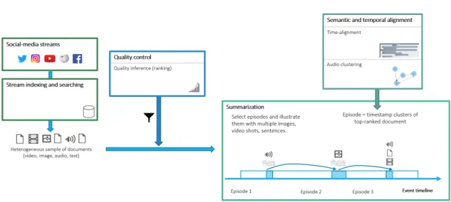
Given the need to handle the vast and heterogeneous social media data, stream in-dexing and searching is an essential starting point of the whole procedure. Next, some filtering is necessary to exclude the data that is not a good representative of a certain event. To achieve this, some quality control has to be performed, which, in the scope of this thesis, can be made through audio inference of a given clip. The end point of this pro-cess is to perform data summarization, where high-quality data related to a certain event must be gathered. For this, temporal alignment is essential since it is the starting point to perform the clustering based on audio cues (i.e., audio clustering). These different steps
are illustrated in figure1.3.
Throughout this thesis we will propose methods that will enabled the quality control step, by inferring the quality of the audio files in a given dataset, and also the semantic and temporal alignment set, by clustering the different audio files in the different existing
events, and by additionally representing how they related with each other in terms of their time offset. A more detailed explanation of this integration steps is further given in
Figure 1.3: Overview of the main project steps, concerning the FCT/UNL work plan.
1.3 Proposed solution
As mentioned above our goal is to analyse and organise user-generated content contain-ing audio cues. Hence, this dissertation focuses on the organisation of different audio
recordings that are relative (i.e.,report) a given event. Considering the use case of this thesis being concert recordings, an event is considered to be a certain concert song. Since it is very likely to exist different recordings of the same concert song, the audio files are
clustered by having common audio segments, with all recordings relative to a given con-cert song belonging to the same cluster in the end. Moreover, the distribution in terms of time of the different recordings throughout the overall event’s timeline is also retrieved.
We also focus on audio quality inference by attributing to each recording a quality score relative to the other recordings in its cluster.
Since the treated audio files are generated from user recordings, some challenges need to be tackled such as the different recording devices possibly used, and the different
qualities inherent to each device. Moreover, it is very unlikely that two recordings are time synchronised and have the same duration. Thus, the development of this work will enable a better comprehension and management of a possibly large dataset of audio files by performing audio clustering and how the different audio files inside each cluster are
distributed over time, as well as a better retrieval of information based on each file’s quality inference.
In practical terms, the quality and clustering information retrieved by our method can be used to organise a list of audio files into the different events represented by the
different clusters (figure1.4), and further aid in the choice of which overlapped recordings
to play to the end-user at a given time based on their quality scores (figure1.5).
1 . 3 . P R O P O S E D S O LU T I O N
Figure 1.4:Grouping of different audio files. Source: [44].
Figure 1.5:Time-aligned audio files. Information about the quality of each file is very useful to choose which one of the audio clips should be played. Source: [9].
synchronisation is required (i.e.,if they are relative to the same event). In our approach, the synchronisation results will serve as the basis to perform the grouping of the files in the different clusters, and enable to know how the different files are distributed over
time in the respective clusters. The audio features used to cluster the data will ultimately help in deriving the quality of each file inside a given cluster. The detailed description of each one of these proposed methods is further presented in sub-sections4.3,4.5, and
4.4, respectively. However, since the synchronisation results that all these methods rely upon might contain false positives, two different filtering approaches are proposed to
filter such false positive matches in sub-section4.6.
Figure1.6describes these methods in a diagram-like view. Starting with a dataset of user-generated audio files, we perform their synchronisation whilst filtering the false pos-itives matches, and we proceed on using the information on the true positive matches to perform the clustering and segmentation of the different files inside each cluster. Finally,
we infer the quality of the different audio files both relative to the rest of the files in their
segments (sub-section4.5.2). The validation of the different proposed methods is given
in Chapter5.
Figure 1.6:Diagram of the different methods needed to achieve the organisation, segmentation, and quality analysis of a large dataset of audio files.
The proposed work will be integrated with other COGNITUS’ working components, more particularly for the ranking of the audio files based on quality score and the group-ing of different audio files representing different events. Important to notice that such
integration mechanisms must be incorporated and developed in the future but are not part of the work presented in this thesis.
Summary of contributions
The main novel contributions of the presented work are considered to be the following:
• Proposal and implementation of two new approaches to detect and filter false posi-tives matches from the audio synchronisation phase. The first proposed approach analyses the derivatives of features derived from the synchronised matches to try to detect sudden drops that might indicate a false positives match, whilst the second uses traditional machine learning classification techniques to classify a match as a false positive or true positive.
• A novel way of inferring audio quality inference of the different audio files relative
to the rest of the files in their cluster and overlapped segments that outperforms the current state-of-the-art.
• The creation of a considerably large dataset of different concert recordings manually
crawled from YouTube containing about 200 recordings across 23 concert songs from different festivals. This dataset was used to further validate and evaluate the
different methods proposed throughout this thesis.
The proposed methods were presented in two different (accepted) scientific papers,
1 . 4 . D O C U M E N T O U T L I N E
1.4 Document outline
This thesis is composed of four chapters:Introduction(chapter1) provides an overview of the objectives and the motivation for the work presented in the upcoming chapters;
Fundamental Concepts(chapter2) introduces some of the concepts that are important to be aware of in order to fully understand the presented work, namely the basics of sound and an introduction to hierarchical clustering;State-of-the-art(chapter3) presents some of the current research state of concerning audio synchronisation and audio clustering;
C
h
a
p
t
e
r
2
F u n d a m e n t a l c o n c e p t s
In order to promote a better understanding of the work and research of this thesis, some concepts are reviewed in this chapter. All the presented information in this chapter can be viewed as a survey of both Yost’s book Fundamental of Hearing [56], serving as an introduction to sound, and the lecture notes of the Machine Learning course lectured at FCT/UNL [23], promoting a better comprehension of the machine learning concepts used throughout this thesis. Hence, readers who are familiar with the concepts described bellow can safely skip to chapter3.
2.1 The basics of sound
In order to produce sound, an object must simply have the ability to vibrate. This ability depends on the properties of inertia and elasticity of each object, that are defined by the force that must be exerted in a given object for it to move and by the ability of that given object to return to its initial state, respectively.
These are the only prerequisites for possible sound production by the direct analysis of the physical definition of sound [56]. In order to achieve actually hearing, the sound wave needs a medium to propagate itself to ultimately be received as input to our auditory system. The pressure changes in the sound wave makes us witness and recognise different
sounds.
2.1.1 Sinusoids
a sinusoid. This particular type of vibration is extremely important since all complex vibrations can be represented as a sum of sinusoids (and therefore also defined as a composition of simple vibrations).
Figure 2.1: Sinusoid relation between displacement and time. Source: [3]
A particular sinusoid is specified by three parameters - amplitude, frequency and starting phase, and, given all vibrations can be defined as a sum of sinusoids, the same parameters apply. Unless all parameters are specified, there is ambiguity since the repre-sentation can correspond to more than one wave.
2.1.2 Sound wave properties
Now, we briefly describe the different parameters that characterise a sinusoid: amplitude,
frequency, and starting phase.
2.1.2.1 Amplitude
Amplitudecan be simply described as a measure of displacement (i.e., how far a certain object moves). Figure2.2shows this measure as simply being the height of the wave.
Figure 2.2: Amplitude representation on a waveform. Source: [28]
2 . 1 . T H E BA S I C S O F S O U N D
waveform, whilstpeak-to-peak amplituderefers to the distance between the maximum positive and maximum negative displacement. These values may be enough in many situations when analysing the amplitude of a given waveform, particularly in the case of periodic waves.
Even though these metrics are useful in some cases, they may give insufficient
infor-mation when analysing the behaviour of complex waves, as the instantaneous amplitude variations cannot be represented in such manner.Root-mean-square amplitudeenables the retrieval of more information about the wave behaviour, by squaring all amplitude values (to turn the negative amplitude values to positives), taking the mean of the squared values, and then taking the square root of the mean in order to go back to the original amplitude scale [54]. Thus,root-mean-square amplitudeis widely used as an amplitude measure since it enables the representation of amplitude in both simple and complex wave forms, like noise. One drawback of this approach is that the calculation of the amplitude in a given moment of time (i.e., instantaneous amplitude) is not possible.
2.1.2.2 Frequency
Frequencycan generally be referred to the measure of how often an object oscillates. This is practically observed as the number of cycles a waveform completes per second, and it is represented byhertz(Hz). Thus, a vibration with frequency equal to 1 Hz means that it takes 1 sec for a wave to complete 1 cycle.
Theoretically, a complete cycle is defined when a vibratory patterns begins and ends at the same point after taking all possible values. The amount of time (in seconds) a vibration takes to achieve a complete cycle is calledperiod. Therefore, frequency and period are intrinsically related as seen in the following equation:
f requency= 1
period
These concepts can also be used to describe complex vibrations, under the condition that they contain some sort of periodic pattern that is repeated. Figure 2.3 shows an example of frequency variation in a sound wave.
2.1.2.3 Starting phase
Starting phaserefers to the initial position of the object relative to the rest position. This is the initial phase of the sinusoid that describes the periodic movement of the object, that is the angle of the sinusoid at time 0 s. The measure is made in terms of degrees of angle and they are all relative to the state observed in the zero degree phase.
Figure 2.4: Sinusoid split in sections of phase in degrees. Source: [41]
When considering a sinusoid, by combining it with trigonometry as explained in [56], a complete cycle can be also represented as 360º. Figure 2.4shows how a sinusoid is divided in different phases. Following this principle, a sinusoid with a phase angle of
270º, starts in the three-quarters before completion of the complete cycle of a zero degree phase sinusoid. This situation is illustrated in figure2.5.
Figure 2.5: Representation of a zero-phase sinusoid (in blue) and a 270º angle phased sinusoid (in pink). Source: [1]
The notion of what the phase would be in any moment of time is calledinstantaneous phase, being the starting phase a particular value of it when t = 0.
2.1.3 Fast Fourier Transform
2 . 1 . T H E BA S I C S O F S O U N D
algorithm than the Discrete Fourier Transform (DFT). Its main practicality is the ability to convert a signal from time-domain to frequency-domain. The inverse can also be done by using the Inverse Fast Fourier Transform (IFFT) algorithm.
FFT serves as the basis for sound processing, since a lot of our perception of sound comes from its frequency-domain representation [56]. This can be easily observed by the ability of humans to identify and be extremely sensitive to changes of the pitch of musical songs, and, consecutively, to changes in the frequency of the audio signal. Pitch is a perceptual measure related to the fundamental frequency, which is the inverse of the period of repetition of complex waves.
2.1.4 Spectrogram
A spectrogram is built from a series ofspectrathat represent the frequency and amplitude of a signal in a moment of time. The stacking of several spectra over a period of time, provide the reasoning behind the creation of a spectrogram. A spectrogram, which is obtained with the Short Time Fourier Transform (STFT), is then a representation of how the spectrum of a certain signal changes over time. Even though STFT retrieves how the phase and magnitude of the signal varies over time and frequency, we will give more focus in the magnitude in this thesis since it consists of one of the features used in relation to frequency in the audio fingerprinting algorithm that will be later described in sub-section3.1.6.
Additionally to the frequency being represented along the vertical axis and time along the horizontal axis, a spectrogram also represents energy in terms of magnitude at a given time and frequency. This is accomplished by a contour map drawn behind the axis nor-mally varying within a colour or grey scale, that is generated from the magnitude valued matrix that represents the magnitude spectrogram. Thus, variations in the energy will produce variations in the background colour, creating a third dimension in the graphic representing the magnitude. Figure2.6shows an example of a spectrogram.
2.2 Classification techniques
The process of predicting the class or category of an example from a finite set of samples is defined as a classification problem in Machine Learning, as illustrate in figure 2.7. This process can either be done by learning from a given set of samples to which the corresponding class is known (i.e., the training data is labelled), or by predicting the classes of new samples without any ground-truth. The first approach is calledsupervised learningwhilst the second is described asunsupervised learning. A merge of the two approaches can also occur, where there is both labelled and unlabelled samples in the training set; this approach is calledsemi-supervised learning.
Figure 2.7: Example of two classification problems. The samples of each class are rep-resented with different colours. On the left, the problem is linearly separable since all
samples of each class can be separated by a line. On the right, the problem is non-linearly separable and another approach had to be used to separate both classes (a circle with radius r). Source: [42]
These different types of learning are closely dependant on the type of problem we are
trying to solve and the type of data we are dealing with. For example, if we have access to a large amount of labelled data and the set of possible labels is knowna prioriand is static, following a supervised learning approach might suffice to achieve good prediction
in the newly classified samples. On the other hand, if we want to derive new conclusions about a large set of unlabelled data, following an unsupervised learning approach suits best our needs.
In the scope of this thesis’ problem we will focus on supervised learning. The features of our data are given as input to the classifier , which will use such features to predict the classes of new samples. Moreover, since we are dealing with labelled data, we can optimise our learning process by making the classifier predict some of the labels of our training samples and compare the its predictions with the corresponding ground-truth label of each sample. However, optimising our classifier to fit and adjust to our training samples might cause overfitting, which is undesirable since it prevents our classifier to generalise to new samples that were not learned in the training phase.
2 . 2 . C L A S S I F I CAT I O N T E C H N I Q U E S
this set), and a test set, to estimate the true error of our model. Since none of the samples in the testing set is used to train our model, we can assume that this estimate is unbiased and therefore a valid measure of evaluation of our predictions. The next subsection (2.2.1) presents a more elegant and better approach to prevent overfitting, and it is followed up by 3 subsections that explain three of the most used methods in the context of solving classification problems with supervised learning.
2.2.1 Cross-Validation
Using the approach of splitting the dataset in training, validation, and testing sets to prevent overfitting is not ideal since it only takes into account one iteration over the ran-domly chosen samples in the different sets, affecting the modelling capability compared
if done iteratively and with a larger amount of samples per set. Moreover, using this ap-proach would also only take into consideration one hypothesis over the several possible hypothesises of our model.
With cross-validation, the samples in the dataset are randomly split intok disjoint folds (beingka number from 2 to the number of samples) and the model is trained with all folds except one, being the left out fold used for validation. This process is repeated for all folds and in the end the average of the validation error of all hypothesis is considered to be the true error of our model. The separation of the samples over the different folds
should preserve the percentage of samples of each class in the original dataset, meaning the folds are stratified. This is important since it maintains the information of the original dataset, that therefore should reflect the real context of our problem.
Using cross-validation is a better approach than simply separating the dataset in 3 (i.e.,training, validation, and test set) since it tests different hypothesis of the model, by
performing several iterations, and therefore by using more data to both train and validate the model since no samples were put aside for the test set. Thus, cross-validation is more likely to produce better predictions and to better generalise our model in the end since different training and validation sets were taken into consideration over the several
iterations.
2.2.2 Logistic Regression
Despite being a regression model, logistic regression can also be used to solve classifica-tion problems. This is easily achieved by finding an hyperplane that separates the two classes where finding an example x of any of the classes lying in that hyperplane has equal probability in both cases.
P(C1|x) =P(C0|x). (2.1)
handling multiple classes one would need to generalise this solution and use Multinomial Logistic Regression but since the problem we tackle in this thesis is a binary classification problem, only two classes will be used and therefore the notions presented will suffice.
This modification is essential when dealing with classification problems since it makes the isolated points located further from the decision boundary to not have a big effect in
its overall position. Thus, the ultimate goal when trying to classify a sample is to simply put it in the correct side of the decision frontier, that will consequently correspond to a correct prediction of its class.
The function used to differentiate the classes is a logistic function, and it can be
directly obtained by the rearrangement of the conditional probabilities based equation (2.1), with its final form being given by:
g(→−x ,we) = 1 1 +e−(
−−−−−−→
wT→−x+w 0)
(2.2)
By being able to receive any real number as input, and outputting a value between 0 and 1, logistic functions are a good way of obtaining a probability of an example pre-viously served as input. Furthermore, logistic functions have the property of varying a lot around a threshold but being nearly constant away from that threshold, as shown in figure 2.8. This is a good feature when dealing with the most further away points and how they affect the output and consecutively the decision boundary position.
Figure 2.8: Example of a Logistic function. Source: [18]
2 . 2 . C L A S S I F I CAT I O N T E C H N I Q U E S
training data. In practical terms, the parametercinfluences the weights of the coefficients
of the chosen hyperplane that separates both classes, as follows:
1
c
m
X
j=i
w2j (2.3)
meaning that bigger vector weights will cause a higher slope, while decreasing the weights will cause a smoother logistic function and therefore less overfitting.
One can use cross-validation to estimate the best value of this parametercby see-ing which model achieves best predictions (i.e., lowest validation error) over the several iterations.
It is important to notice that this is a linear classifier, since it simply tries to find an hyperplane that divides the two classes. Therefore, if the classes are not linearly separable by default this classifier will suffice in correctly setting its decision boundary. To handle
this problem we can increase the dimensions of our features (i.e., we can either try to find more independent features of our samples or combine the existing features into new, dependant, ones). By increasing the feature space and consecutively increasing the computational power as a drawback, it is then possible for our linear classifier to correctly separate our training data.
2.2.3 K-Nearest Neighbours
Instead of fitting a model based on the samples in the training set, the K-Nearest Neigh-bours classifier simply compares never seen samples to the samples of the training set. The basic idea is that a new sample is given the same class of the majority of theknearest samples in the training set (beingkan odd number between 1 and the number of samples in the training dataset). A smallkis more likely to promote overfitting, whereas a large
kpromotes underfitting (see figure2.9). Thus, it is important to find the best number of neighbours by applying cross-validation, similarly to what was already described when choosing thecparameter of the Logistic Regression classifier.
Figure 2.9: Comparison of using a different number of neighbours for the classifier (1, 13
Since this is a distance-based method, a distance function must be chosen to calculate the closest training sample points to the new sample point in the feature space. Euclidean distance is the most used but another distance metrics might produce better results in specific problems, such as the Minkowsky distance for continuous numerical features, and the Hamming distance for categorical features [23].
Unlike the logistic regression classifier, increasing the dimensional space of our fea-tures will not necessarily produce better predictions when using the K-Nearest Neigh-bours classifier. This is inherent to any distance-based classification method since more dimensions normally mean points are more distant of each other and so are their neigh-bours, meaning that the class of the majority might be incorrect and wrongly predicted for a new sample. Thus, when dealing with high dimensional feature spaces and a high value ofk, it might be better to analyse the distance of the points, by introducing a weight based on the distance metric [43]. This way closer neighbours would influence more the class prediction than the furthest neighbours.
2.2.4 Support Vector Machines
Similarly to the Logistic Regression classifier, Support Vector Machines (SVM) finds a hyperplane that separates two classes, assuming that the classes are indeed linearly sepa-rable. The main difference, however, is that with SVM the chosen hyperplane is the one
that maximises the distance between the two classes. This solves an important problem of Logistic Regression, that consists of allowing the frontier to be closer to some points of a given class than the others. This is originated by the logistic function being almost flat away from the frontier, making small differences in the position of the decision boundary
to not make any difference in the overall result. This results in the frontier being placed
in a different position when we run the Logistic Regression Classifier several times, as
shown in figure2.10.
Figure 2.10: Different runs of the Logistic Regression classifier result in different positions
2 . 2 . C L A S S I F I CAT I O N T E C H N I Q U E S
To maximise the margin between the frontier and classes, we look in the distance between the closest points of each class and the frontier (such points are represented in a vector form and described as support vectors). The goal is therefore to maximise the distance between the support vectors and the decision hyperplane, as demonstrated in figure2.11. The chosen hyperplane can be formally defined as:
g(→−x) =→w−T→−x +w0 (2.4)
where→−w represents a vector of weights andw0the bias. This function, when served with
an input vector (i.e., one sample), returns values greater or equal than 1 for one class and values smaller or equal to -1 for the samples of the other class.
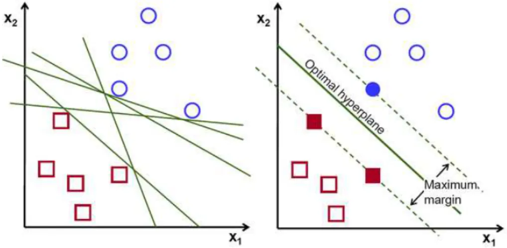
Figure 2.11: On the left, different possible hyper planes that successfully separate both classes are shown. On the right, only the hyperplane that had the maximum margin from the closest points of each class (denoted as support vectors). Source: [37]
The absolute value of the output of the function represents the distance from the input vector to the hyperplane, being this distance equal to 1 if the input vector is a support vector. Since the shortest distance between a point and a hyperplane is defined by:
d=|g(
− →x)|
|| −→w|| (2.5)
and for support vectors|g(→−x)| is equal to 1, one can maximise the margin between the frontier and the support vectors by minimising|| −→w||. This is a non-linear optimisation task that can be solved by using Lagrange Multipliers [45].
slack variable then represents the distance between a vector and the inside margin of the hyperplane.
By introducing the slack variables to each vector, we allow some points to fall on the wrong side of the margin by introducing a certain penalty to them. These penalties are upper bounded by the regularisation parameterc, meaning a high value ofca high penalty for margin violation, with no support vectors being placed inside the margins, whereas a low value ofcwill allow several points to be placed in the wrong side of the hyperplane. This idea is illustrated in figure2.12.
Figure 2.12: Different values ofcwere used for different runs of the SVM. For the left image a
cvalue of 1 was used, where it is visible several support vectors being placed inside the margins (outlined with red circles), whilst in the right imagecwas equal to 1000 and no margin violations are observed. Source: [23]
Allowing some errors in the decision frontier might not work if there is too much overlap between both classes. In this case it is preferred to increase the dimensions of the feature space, as previously discussed. Increasing the number of features in SVM is considerably easy since we are only concerned about performing the inner product operations between the extended featured vectors. This operations can be done by using kernel functions, that return the inner product of the transformed vectors as a function of the original dimensional vectors. This is done by using an auxiliary function that adds dimensions to the original vectors (e.g., receives a 2-dimensional vector and returns a 4-dimensional vector).
Different kernel functions (e.g., linear, polynomial, Gaussian) can be used and tested,
with the Gaussian Radial Basis Function (RBF) being normally set as the default kernel to use in non-linear solutions, since it maps the training examples into a higher dimensional space. Important to notice that this kernel has the same performance as a linear kernel using the right combination of parameters, and it is less complex than the polynomial kernel, since it uses less hyper parameters to select the best model [20].
2 . 3 . H I E R A R C H I CA L C LU S T E R I N G
decision frontier [23]. A good way of finding the right combination of this two parameters (i.e.,candγ) is to execute an exhaustive search over all possible combinations of a subset of possible values for each parameter, also described as grid-search. This process can be optimised by using cross-validation, choosing the pair of parameters’ values that had the highest mean accuracy in the different folds.
2.3 Hierarchical Clustering
If we wish to organise and group samples together based on a certain similarity, we are dealing with a Clustering problem. One approach to decide the right number of clusters in a big dataset, is to do it in an iterative manner by joining first the samples that are more similar and then gradually merging similar clusters. This approach is called hierarchical clustering and is illustrated in figure2.13, where the letters "a" to "f" are isolated and then are iteratively combined to form the combination "abcdef".
Figure 2.13: Example of hierarchical clustering. Source: [52]
This type of clustering suggests that is not only needed to find measures of similarity between samples, but also between clusters, so they are rightfully merged. These cluster measures can be represented by a simple Boolean value, where 1 indicates that two clus-ters are similar and 0 the opposite, or by more complex measurements like the distance between clusters. There are a lot of ways to perform the calculation of this distance (for more details see [23]). In this work the measure of similarity is set to be a Boolean, since that is what suits the best to our problem and presented solution.
Hierarchical clustering can be done by either starting with singleton clusters and proceed on merging similar clusters (i.e., agglomerative clustering) or by following a top-down approach, where a single cluster with all examples is formed and then iteratively split into smaller clusters (i.e., divisive clustering). Figure 2.14 shows an example of agglomerative clustering, where initially all samples are separated (i.e., forming singleton clusters), and then are grouped together until they are all gathered in the same cluster.
Our proposed solution uses an adaptation of agglomerative clustering to group audio samples from music concerts into different clusters (section 4.3). It is an adaptation
fingerprinting algorithm described in subsection3.1.6. This idea of the audio clustering process will be firstly introduced in section3.2and practically described with detail in chapter4.
Figure 2.14:Example of agglomerative clustering. Source: [51]
Concluding remarks
In this chapter we introduced some basic concepts of sound that will enable a better understanding of the features used by the audio fingerprinting techniques that will be further explained in the next chapter. Moreover, machine learning methods together with some important supervised learning notions were also introduced. All the introduced concepts in this chapter create an important basis for the formulation of the different
C
h
a
p
t
e
r
3
S t a t e - o f - t h e -a rt
In this chapter we present the state-of-the-art work by the time this research work be-gan. We survey the different processes inherent to an audio fingerprinting algorithm,
(section3.1) and give more detailed information about the algorithm that was used in the actual implementation phase of this work. Furthermore, we introduce previous work that served as the basis of the different proposed methods in this thesis, focusing mainly
on audio clustering (section3.2).
3.1 Audio fingerprinting
The synchronisation of different audio files is an essential step to perform the audio
clus-tering, since it is the mechanism used to group different files with common overlapping
segments. Moreover, the information about the different audio files are distributed
over-time inside a given cluster is made through the offset between the different samples. To
derive the quality of the different files inside a given cluster, information about how the
synchronisation process happened is also essential for the proposed method. The detailed explanation of these processes, and the different approaches that can be followed, can be
found in sections4.3,4.5, and4.4, respectively.
Audio Fingerprinting techniques are often used to perform the synchronisation be-tween audio files by the usage of audio features that are relatively resistant to noise. This represents an ideal background to perform the synchronisation of our data since it en-ables to synchronise noisy samples against possibly less noisy audio files in the database, while only needing possibly short length common segments to synchronise both clips.
While audio fingerprinting has traditionally been used for song recognition, as made famous byShazambut also other existing applications, such asMidomi[30],Chromaprint
relatively new ([22] is further analysed in section3.2). In the latter case, instead of using the offset retrieved from the audio fingerprinting to align the audio files, that offset will
serve to conclude that the files have a common segment and therefore should be simply put in the same cluster.
Fingerprint generation over any kind of data is an efficient mechanism to characterise
possibly large data with a small representation. More explicitly, as an alternative to rep-resentations that involve large amounts of data, fingerprints are compact reprep-resentations of the data that can be used for purposes that do not require dealing with all the intrinsic details of the data. This technique promotes a fast way of comparing the quality of two entities by trying to diminish the need to compare irrelevant features.
Any audio fingerprinting technique involves an extraction mechanism to generate the fingerprints of data and then a searching mechanism that looks for matching fingerprints in a pre-generated database. Different audio fingerprinting algorithms (such as [13,16, 50]) can be compared based on theirrobustness(i.e., how well the algorithm performs with additive noise), reliability(i.e., the probability of having false positives), search speed(i.e., how fast the algorithm can identify a match) andscalability(i.e., how well the algorithm performs with a large database).
The variety of these benchmarks differ on how the algorithm is implemented and
how the fingerprints are generated. Therefore, they are intrinsically associated with the chosen size of the fingerprints used, since it will directly influence the storage needed and search speed of the algorithm, and how many seconds are needed to identify a certain song (i.e., granularity).
There are several steps inherent that have to be complete to achieve the match between two audio files. First, an extraction of some of the features present in the audio clip has to be done; second, those features, or a combination of them, are then used to generate a fingerprint that will characterise the audio clip in question; then, searching processes must be applied to access the fingerprints of the other files in the database; and finally matching mechanisms have to be performed to compare pairs of fingerprints and generate a match. Each one of these steps is explained with more detail over the next subsections.
3.1.1 Features extraction
How the fingerprints are generated from the features extracted from the audio signal is one of the main points of the choice of the audio fingerprinting algorithm to use. Some principals are inherent to almost every existing fingerprinting algorithm, such as splitting the audio signal in smaller pieces, and then proceed to extract features of such smaller sized portions. Regarding the first step, the splitting decision is on how tiny such frames will be, since excessive divisions can put an unnecessary computing power on the creation of the fingerprints, and a low number of divisions can suffice to create an
efficient fingerprint representation.
3 . 1 . AU D I O F I N G E R P R I N T I N G
invariant to signal degradation such as: Fourier coefficients, with different and less
com-putational expensive ways of calculating the Fast Fourier Transform (FFT) over the same samples [15]; Mel-Frequency Cepstral Coefficients (MFFC) [25], that have into the
con-sideration the energy representation of the audio signal; statistics of features retrieved from Discrete Fourier Transform at each instant of time [4]; and several others amplitude driven methods as referred in [12].
Although each one of the extraction methods could be more beneficial to use depend-ing on the context, it is known that most important features used by the auditory system to perceive sounds live in the frequency domain, as stated in [16] and already mentioned in subsection 2.1.3. Thus, algorithms that use Fourier Transform are preferable in the majority of the cases.
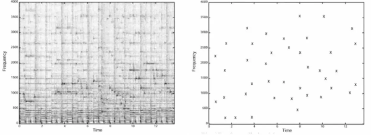
In order to illustrate an example of the features extraction process and how it simpli-fies the data representation, figure3.1 represents the output of the features extraction used inShazam[50]. In this case, the extraction is made through the selection of frequency peaks in the spectrogram of a given audio signal. This procedure is better explained in subsection 3.1.6, since the fingerprinting algorithm that ended up being used in the implementation phase is also inspired in this peak extraction concept.
Figure 3.1: A spectrogram (in the left) with the correspondent extracted features on the right. Source: [50]
3.1.2 Fingerprint generation
After extracting the features from the data, the next step in any fingerprinting algorithm is to use such features to produce the hopefully correct and singular representation of the respective audio file. This generation process varies from different algorithms but in
of an audio clip is called sub-fingerprint, as introduced in [16]. Thus, one fingerprint can be seen as an aggregation of several sub-fingerprints.
These sub-fingerprints can be calculated not only using the raw values of the extracted features but also by performing combinations between such features, in order to promote a more unique representation of a given file. The way to relate features is therefore extremely important, since it might reduce the need of consider all extracted features but simply focus on their relation during certain periods of time.
One effective way of performing these combinations between single features was
pro-posed byShazam in [50]. Considering the peaks extracted in figure3.1, the algorithm makes combinations between them to produce more detailed information about that au-dio file. This process is accomplished by choosing anchor points, that consists of a subset of points uniformly distributed in the set of the extracted peaks, and then combining each anchor point with other peaks inside a target zone, in a sequential way. This first part of the overall fingerprint generation process is illustrated in the left part of figure
3.2.
Since these peaks were retrieved from spectrogram, information about their frequency in a given moment of time is available. Thus, this combination is passed as input to a hash function, by giving the frequencies of both peaks and the time difference between
them. This will result in a hash representation of that information (32-bit), ultimately consisting the sub-fingerprints of an audio file. This is demonstrated in the right part of figure3.2. This whole process is then repeated for each anchor point, and then the list of all hashes will be used to characterise an audio clip, forming its fingerprint.
Figure 3.2:Description of the hash generation process inShazam. Source: [50]
3.1.3 Robust audio hashing
The hash functions used in summarising audio data are based on a different notion than
3 . 1 . AU D I O F I N G E R P R I N T I N G
data is extremely fragile in the meanings of a very subtle difference on the content will
result in a completely different hash value.
In the case of audio, there is a need to use a threshold since the audio files can be sub-ject to degradation factors possibly originated by compression or conversion mechanisms. Thus, hashes of audio content imply that different quality versions of a given audio clip
are given the same hash, as stated in [38] and [48]. This type of hashes are calledrobust hashes.
This is practically observed in the output of the fingerprinting algorithm described in subsection3.1.6, where different versions of audio files are matched depending on the
query file to match. This is shown by the display of how that version ranks in all hashes of that song.
This method of hashing audio content is widely used in audio fingerprinting, as op-posed to audio watermarking [11] where some kind of signature is embedded in the original content before its release. Even though this technique is very useful in detecting copyright problems [17], it suffices to work in the context of our problem.
3.1.4 Searching process
Giving the likely abundance of audio files in the database, both when dealing with mu-sic recognition applications and data retrieved from social media websites, an efficient
way of searching must be implemented. The size of the database is even more problem-atic considering that each song’s fingerprint is composed by several bits of information representing the sub-fingerprints.
An extensive search of the entire database is not practical [16], especially when the response time matters which is a common requirement in most real-world applications. Thus, approaches for reducing the number of records to be accessed and/or strategies to optimise the way the information is saved and accessed must take place.
Such approaches vary in whether the information is indexed based on sub-fingerprints, which usually infers an exact match from the database (e.g., searching of hash matches), or based on fingerprint-blocks, that consist of the whole information that characterises a given clip. This last approach normally infers that a similar match is needed and not an exact match, since two different clips with exactly the same fingerprint are unlikely to
happen even if they represent different recordings of the same song.
When considering sub-fingerprint indexing, data structures used to store the infor-mation normally consist of hash tables ([16]), inverted index hash tables ([10]) or tree-structured based representations ([55]). These ways of representing the sub-fingerprints enable for a sparse representation of the information, therefore promoting practicability and an efficient way of searching [16].
building classes to group similar fingerprints ([7]) or inferring the similarity probability of a candidate ([16]).
3.1.5 Matching process
After obtaining the fingerprints, it is important to understand whether a match between two different clips is found or not. This decision process can be easily performed by
following the methodology that if two clips have common sub-fingerprints (e.g., hashes), then there exists a match between them. A minimum amount of matching hashes is normally taking into account to prevent false positives.
The matching process can be generalised as simply analysing the offset between the
matching hashes of the clips that are being compared. This is done for every clip in the database, and clips with a sufficient number of matching hashes (usually a small number
since the unlikeliness of false matches) over a given offset are considered to be a match
relative to the query song.
This process can be practically achieved by the creation of bins for each audio file matched, with the added information of the offset between the two files. Thus, a bin is a
representation of all the different matching hashes of a certain song in the database over
several offsets. To identify the most frequent offsets of the different hash matches, one
can generate a scatter plot of the different matches over time and check for diagonal lines
as they indicate the same offset over different matches. This is illustrated in figure3.3.
Another way of identifying that frequency is simply by using a histogram and proceed to find relevant peaks (figure3.4).
Figure 3.3:Scatter plot of the timestamps of the different matches. Source: [49]
![Figure 1.2: User-generated Content creation. Source: [8]](https://thumb-eu.123doks.com/thumbv2/123dok_br/16532277.736343/22.892.222.672.689.892/figure-user-generated-content-creation-source.webp)
![Figure 2.6: Spectrogram captured of a recording of some words. Source: [53].](https://thumb-eu.123doks.com/thumbv2/123dok_br/16532277.736343/33.892.191.703.846.1107/figure-spectrogram-captured-recording-words-source.webp)
![Figure 2.8: Example of a Logistic function. Source: [18]](https://thumb-eu.123doks.com/thumbv2/123dok_br/16532277.736343/36.892.257.637.687.943/figure-example-logistic-function-source.webp)

![Figure 3.2: Description of the hash generation process in Shazam. Source: [50]](https://thumb-eu.123doks.com/thumbv2/123dok_br/16532277.736343/46.892.133.762.727.973/figure-description-hash-generation-process-shazam-source.webp)
![Figure 3.3: Scatter plot of the timestamps of the di ff erent matches. Source: [49]](https://thumb-eu.123doks.com/thumbv2/123dok_br/16532277.736343/48.892.143.762.798.1005/figure-scatter-plot-timestamps-di-erent-matches-source.webp)
