Todos os direitos reservados.
É proibida a reprodução parcial ou integral do conteúdo
deste documento por qualquer meio de distribuição, digital ou
impresso, sem a expressa autorização do
REAP ou de seu autor.
Family Planning and Development:
Aggregate Effects of Contraceptive Use
Tiago Cavalcanti
Georgi Kocharkov
Cezar Santos
Family Planning and Development:
Aggregate Effects of Contraceptive Use
Tiago Cavalcanti
Georgi Kocharkov
Cezar Santos
Tiago Cavalcanti
University of Cambridge and EESP/FGV-SP
Georgi Kocharkov University of Konstanz
Cezar Santos EPGE/FGV-Rio
Family Planning and Development:
Aggregate Effects of Contraceptive Use
∗
Tiago Cavalcanti
University of Cambridge and EESP/FGV-SP
Georgi Kocharkov
University of Konstanz [email protected]
Cezar Santos
EPGE/FGV-Rio [email protected]
Abstract
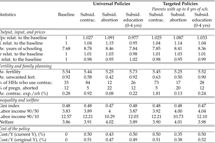
What is the role of family planning interventions on fertility, savings, human capi-tal investment, and development? To examine this, endogenous unwanted fertility is embedded in an otherwise standard quantity-quality overlapping generations model of fertility and growth. The model features costly fertility control and families can (partially) insure against a fertility risk by using costly modern contraceptives. In the event of unexpected pregnancies, households can also opt to abort some pregnancies, at a cost. Given the number of children born, parents decide how much education to provide and how much to save out of their income. We fit the model to Kenyan data, implement several family planning policies and decompose their aggregate ef-fects. Our results suggest that given a small budget (up to 0.5 percent of GDP), legaliz-ing and subsidizlegaliz-ing the price of abortion is a more cost-effective policy for improvlegaliz-ing long-run living standards and reducing inequality than policies that either subsidize the price of modern contraceptives or subsidize basic education.
KEYWORDS: education, income per capita, contraception, abortion
JEL CLASSIFICATION: E24, I15, J13, O11.
∗We have benefited from discussions and conversations with Kenneth Arrow, Oded Galor, Jeremy
“Each family tries to come as close as possible to its desired number of children... Families with excess children consume less of other goods, especially of goods that are close substitutes for the quantity of children. Because quality seems like a relatively close substitute for quantity, families with excess children would spend less on each child than other families with equal income and tastes. Accordingly, an increase in contraceptive knowledge would raise the quality of children as well as reduce their quantity.” (Becker,1960, p. 218)
1
Introduction
What is the role of family planning interventions on fertility, savings, human capital in-vestment, and development? SinceMalthus(1798), population dynamics have been at the core of long-run economic analysis, and recent growth models (cf.,Galor and Weil,2000) have continued to emphasize this. A common view in economic growth theory is that high fertility mainly reflects desired family size and that parents are able to achieve their fertility target (cf., Barro and Becker, 1989). From this perspective, fertility changes are driven by parents’ demand for children (e.g., quantity-quality substitution or declining infant mortality) and supply factors, such as family-planning interventions, should have no impact on family size. However, in reality, sometimes people want to have the chil-dren they conceive, and sometimes they do not. Though this statement may sound rather terse, there is evidence to back it up.1 According to Bongaarts (2016) about 39 percent of annual developing-world pregnancies are unplanned, and roughly half of these end in induced abortions. In fact, in some countries, there is quite a substantial gap between ac-tual realized fertility and wanted fertility; and this gap is also larger for relatively poorer households. The fact that contraceptive methods are costly and individuals sometimes re-sort to abortions in order to control their family sizes corroborates this idea. In sum, there seems to be a random aspect to fertility.2
When parents have children, a natural step that follows is to provide them with care and education. Needless to say, while children bring a variety of inestimable benefits to parents, they are costly both in terms of goods and time. For instance, education costs money: tuition fees, books, transportation, and foregone wages that could come from child labor. Education and childrearing are also costly in terms of time: parents usually transmit their values, religion, and culture to their children, and parents must furthermore take care of their children when they are sick.
When added together, the statements in the previous two paragraphs (i.e., the ran-domness of fertility and the cost of child care and education) imply that the educational attainment of children in practice may not be as high as in a situation in which parents
1We provide detailed empirical facts on this issue in Section2.
2This is emphasized inMalthus(1798) in a time when modern contraceptive methods were not
could perfectly control their fertility (cf.,Becker, 1960). In the aggregate, this may imply that human capital may be lower due to the randomness of family size. In addition, if poor households have lower control of their family size, this can lead to more heterogeneity in fertility with consequences on the level and persistence of inequality in education and income.3 This could also have an effect on a country’s production output since workers will have lower skills. The natural question is whether or not such effects are important and how family planning interventions affect the fertility gap. This paper addresses these questions.4
Although the ability to control family size is present even in primitive societies through abortion, infanticide, and other practices, and some very effective contraceptive methods have been available for more than 100 years (cf., Himes, 1936), there still exists a gap between realized and desired fertility in developing countries (see Table8 in Appendix
A). In addition, this gap is negatively correlated with income (see Table 9 in Appendix
A). For instance, the proportion of women with unmet need for contraception could be as high as 40 percent in the Democratic Republic of Congo (cf.,The World Bank,2010) and it is in general higher for low income households.5 The empirical evidence also shows that there exists a significant negative relationship between the fertility gap and educational attainment across countries. That is, when fertility is closer to its desired level, educational attainment is higher. Moreover the fertility gap is lower in countries where contraceptive use is more widespread.6 This last correlation holds even when country-fixed effects, which control for main religion and other cultural factors, and the level of development are taken into account (see Table1). In some ways this is, at least for us, a surprising fact.
We develop a general macroeconomic equilibrium model to assess the questions above. The model economy is populated by overlapping generations. Households make a con-sumption and savings decision and imperfectly choose how many (quantity) children they want to have (demand factors). However, households may have more pregnancies than desired due to unexpected fertility shocks. Families can partially insure against this fer-tility risk by using costly contraception (supply factors). In the event of unexpected preg-nancies, households can opt to abort some of the time, and abortion is also costly. Given the number of children born, parents decide how much (quality) education to provide them. Schooling is costly in terms of consumption goods and children rearing is costly in terms of the time. These features allow us to map indicators (e.g., the contraceptive
3Using data from Quebec from the 16th to the 18th century,Galor and Klemp(2015) also explore the
absence of reliable contraceptive methods in the determination of fertility to show that moderate fecun-dity and thus predisposition towards investment in child quality was conducive to long-run reproductive success, reflecting the negative effect of higher fecundity on the education of each offspring.
4It is important to stress that this is not necessarily a paper about an overpopulation problem (cf.,Ehrlich
and Ehrlich,1990;Easterlin,1987). Family planning interventions may be justified even when the overall
fertility rate is below the replacement rate, but when some households have a fertility rate above their desired level.
5The median for developing countries is 22 percent. According to this World Bank report, the definition
of unmet need for contraception corresponds to the “proportion of currently married women who do not want any more children but are not using any form of family planning or currently married women who want to postpone their next birth for two years but are not using any form of family planning”.
prevalence rate, abortion rate, unwanted fertility, and unmet need for family planning) of reproductive behavior from the data into the model and to study different family planning interventions. On the production side of the economy, there is a standard representative firm which uses labor and capital as inputs to produce final goods. We solve for a station-ary equilibrium.
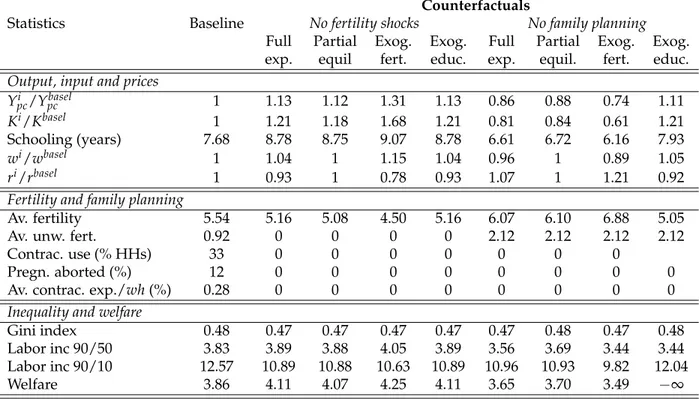
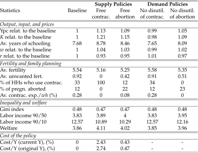
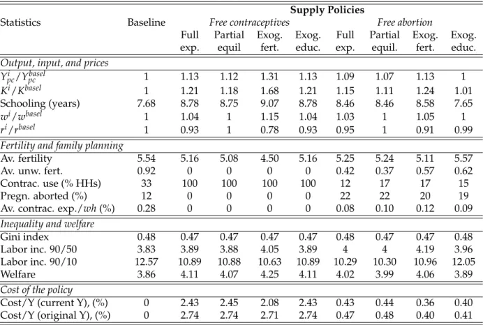
The model parameters are fitted to match statistical moments from the Kenyan econ-omy, a country in which the average fertility gap is 1.2 children, which is above the average (0.87) for all developing countries in our dataset. The average gap hides important hetero-geneity since the gap between realized and wanted fertility is about 2 children for parents with a primary degree (8 years of schooling) and 0.6 for parents with more than 12 years of schooling. In the baseline economy there is substantial heterogeneity in education and income. In particular, we are able to replicate the fertility pattern (levels and heterogene-ity) and fertility gap observed in the data. The benchmark model is then used to assess the importance of family-planning interventions on education, inequality, and income per capita. Counterfactual exercises are implemented to shed some light on the quantitative importance of contraception use. For instance, in a world without fertility risk (i.e. with no unwanted pregnancies), educational attainment would be higher by about 1.1 extra year of education. Together with a rise in the capital stock, this leads to a hike in income per capita of about 13 percent. We also investigate several policies commonly used, includ-ing policies targeted at the poor. We show that given a small government budget (say 0.5 percent of GDP), legalizing and subsidizing the price of abortion is the most cost-effective policy in improving living standards when compared to policies that subsidize either the price of modern contraceptives or education.
We also decompose the full effect of family planning interventions on the economy into three different channels: a general equilibrium effect due to price movements, a wanted fertility channel since desired fertility may change with policies, and the response of par-ents investment in education of their children. We show that to fully understand the ef-fects of family planning policies on individual outcomes it is important to perceive the responses of households in terms of desired fertility to individual policies, as well as the interaction of these responses with households investment decisions. For instance, fami-lies target a higher wanted fertility rate when the fertility risk of unwanted pregnancies is reduced. This can mitigate some of the effects of family planning policies on reproductive behavior, investment, and income levels.
Our research is related to a large literature on the relationship between fertility and development. Most of the papers in this literature focus on the joint evolution of eco-nomic and demographic processes (cf.,Barro and Becker, 1989; de la Croix and Doepke,
2003;Galor and Weil, 1996,2000) represented by a negative relationship between fertility and income.7 The main idea is that when income rises the opportunity cost of raising children rises and parents decrease their family size and invest more in each child (cf.,
Becker, Murphy, and Tamura,1990). This is the quantity-quality trade-off, which depends
7Our model can generate a negative correlation between fertility and income even when the desired
on the income elasticity of the quantity and quality of children, postulated and explained intuitively by Becker (1960), which has been the dominant theoretical framework in the economics of fertility over the past decades (cf.,Doepke,2015). Economists have used this framework to understand the dynamics of economic development and whether or not fer-tility choice can help to explain such dynamics.8 For instance, de la Croix and Doepke (2003) discuss the importance of differential fertility for development through the educa-tion channel, a channel that is further explored inVogl(2016) and which is also important in our paper. However, unlike our work, most of these articles do not focus on costly contraceptive methods, fertility risks, and family intervention policies.Becker(1960) does discuss in detail the importance of contraceptive methods in controlling family size, but birth control techniques are not mentioned in his subsequent work (cf.,Barro and Becker,
1989;Becker and Lewis, 1973).9 Our interpretation is that the discussion of most of these articles focus on fertility in developed countries, such as the United States, where these contraceptive methods are affordable and readily available to the public. In addition, there is public awareness about their effectiveness in controlling pregnancies, and therefore the realized number of children is very close to the desired one. Our view is that this might not be the case for some developing countries, and this view seems to be backed by the empirical evidence. In developing countries even when contraceptives can be obtained at low cost in public clinics , for example, they are often stocked out. Ashraf, Field, and Lee
(2014) report a survey conducted by the United States Agency for International Develop-ment (USAID) between October and December 2007, in which it was found that more than half of the hospitals and health clinics in Zambia were stocked out of injectable vaccines (and pills) for more than 50% (30%) of the 90 days over which the survey was conducted. To our knowledge our paper is the first to consider explicitly costly contraception choice in a model of growth and development with endogenous population growth. Baudin, de la Croix, and Gobbi (2016) also consider unwanted fertility by assuming that a share of couples cannot control fertility, but this differs from our approach since we assume that fertility control is costly and the lack of ability to perfectly control pregnancies is de-rived from economic incentives.10 They investigate a family planning policy which sets the percentage of couples able to control their fertility to one.11 Ashraf, Weil, and Wilde (2013) also study the effects of policies which reduce fertility on investment and output per capita. Fertility is exogenous in their framework and they feed different population dynamics into a growth model to investigate how each affects output through different
8The model has also being used to understand a variety of related issues (cf.,Doepke and Zilibotti,2005;
Greenwood, Seshadri, and Yorukoglu,2005).
9Doepke(2015) states that “In the sense that the lack of knowledge of birth control among poorer
house-holds is assumed rather than derived from economic incentives, Becker’s 1960 paper does not yet go all the way in founding fertility choice in economics.” We provide economic foundation for that based on costly contraceptives and we show that this may be quantitatively important in some developing countries.
10The authors also take fertility risks into account by assuming that the number of children who survive
to adulthood within a family is a random variable. This approach is also taken bySah(1991) and
Kalemli-Ozcan(2003).
11In their quantitative exercises, the authors show that abstracting from the extensive margin in fertility
channels. In our case, fertility and the use of costly contraceptive methods are endoge-nous. This allows us not only to evaluate the effects of family planning interventions on output but also to show how the use of contraceptives, and thus fertility, changes along with other policies such as investment in education.
Our general idea relies on the assumption that family planning interventions have a first-order effect on fertility decisions. There is a bulk of evidence supporting this. See
May(2012) andSchultz(2008), among many others. For instance,Bloom, Canning, Fink, and Finlay(2009) show that removing legal restrictions on abortion significantly reduces fertility and that this has a positive impact on female labor force participation. Joshi and Schultz(2013) study the long-run consequences of a randomized control trial of contra-ception provision in Matlab, Bangladesh. Their findings suggest that treatment villages experienced a decline in fertility of about 17 percent compared to control villages, and that the effects were persistent over a 20-year period. Sinha(2005) estimates similar effects of this family planning experiment on fertility. Using an experiment in Zambia, Ashraf, Field, and Lee(2014) show that the local average treatment effect estimation implies that use of family planning services during about two years of the experiment was associated with a 27 percent reduction in births. Using variation in the timing and location of the Profamilia program in Colombia, Miller (2010) finds that availability of modern contra-ceptives allowed women to postpone their first birth and to have about 5 percent fewer children in their lifetime.12 Banerjee, Meng, Porzio, and Qian (2014) estimate the effects of birth control policies in China before the “one-child policy’. They show that family planning reduced fertility and increased savings. Our model helps to rationalize these findings since we integrate demand and supply factors in the determination of fertility, which is not possible in a standard quantity-quality fertility model.13 This paper therefore provides a bridge between the macro literature on fertility and growth and the empirical micro literature on family planning interventions, fertility, and human capital outcomes. In addition, with our framework it is possible to run and to evaluate a variety of counter-factual policies, not necessarily available in control trial experiments, and to disentangle different channels, such as the importance of general equilibrium effects. Therefore, we believe our paper is an important contribution to the literature on family planning policy and development, filling an existing gap with far-reaching implications for policies.
The remainder of this paper is divided into six additional sections besides this
intro-12There is also a branch of the literature which focuses on different effects of fertility risk. Some examples
areGoldin and Katz(2002) andEdlund and Machado(2015), which discuss the impact of the (availability
of the) pill on several dimensions of women’s education and careers. They do so for the US and without a focus on aggregate development, but they show that the diffusion of the pill had a first-order effect on the education of women and on the decision to marry.Kocharkov(2014) studies the relation between abortions and inequality. He also focuses on US data and, unlike our work, does not discuss aggregate impacts.
Choi(2017) introduces fertility risk in a life-cycle model with consumption, savings and fertility decisions estimated for the US. He shows that differential fertility risk is essential in generating plausible life-cycle patterns of births and abortions across educational groups.
13This is different from the “one-child policy” in China. Related to our work,Choukhmane, Coeurdacier,
and Jin(2016) show that this policy led to an increase in the savings rate and human capital accumulation
duction. In order to motivate our study, some empirical facts are documented in Section
2. Section 3 presents a simplified version of the model to provide some key intuition and analytical results. Section 4 describes the model economy, which is used for quan-titative analysis. Section5 fits model parameters to the data, and Section6 provides the quantitative analysis to measure the aggregate effects of family planning interventions on development. Section7contains concluding remarks.
2
Facts
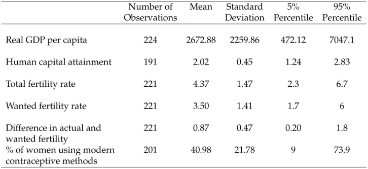
In this section we describe the empirical facts which motivate our work.14 Table1shows the regression results in which the dependent variable is the unwanted fertility, or the gap between actual and wanted fertility, and the explanatory variable of interest is the percentage of women who have ever used modern contraceptive methods. We have an unbalanced panel since the Demographic Health Surveys from USAID, which contain in-formation on the fertility gap and contraceptive use across countries, are implemented in countries on different dates. There are 84 countries in total, but they appear in the sample in different frequencies and in years ranging from 1985 to 2010. Before we proceed with the analysis, it is important to emphasize up front that we do not aim to provide a causal effect of modern contraceptive use on the fertility gap, instead focusing on examining the relationship between the two. We are aware of issues related to unobservables which can drive the correlations between these two variables and reverse causality problems.15
Column (1) of Table 1 presents the estimated coefficients when we regress the fertil-ity gap on the logarithm of per capita income and the percentage of women who have ever used modern contraceptive methods. As we can see, there is a negative associa-tion between unwanted fertility and the measure of modern contraceptive use, but this correlation is not statistically different from zero at the usual confidence levels. This neg-ative correlation becomes statistically significant once we introduce country fixed effects, which control for time invariant effects such as legal origin, main religion, and other cul-tural factors. Notice that country fixed effects substantially increase the explanation of the observed variation in the fertility gap. According to specification (2) the gap between realized and wanted fertility is significantly lower in countries where contraceptive use is more widespread. Quantitatively this regression implies that an increase in one stan-dard deviation (22 percentage points) in the percentage of women who have ever used modern contraceptive methods is associated with a decrease in the fertility gap of 0.22 of a child. The regression in Column (3) contains the same explanatory variables as the one in Column (2) but we also introduce dummies for each decade.16 The correlation between
14The descriptions of all data sources, summary statistics, and simple correlations are reported in
Ap-pendixA.
15Ideally we would instrument the use of modern contraceptive methods. One possibility would be to
use the relative price of modern contraceptive methods (e.g., pills and condom) as an instrumental variable for the fraction of women who have ever used modern contraceptive methods, but we were unable to find historical data for this variable for the majority of countries.
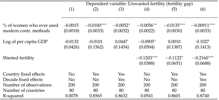
Table 1: Relationship between unwanted fertility and the use of modern contraceptive methods. Data source: see data appendix for description and source of the variables used.
Dependent variable: Unwanted fertility (fertility gap) (1) (2) (3) (4) (5) (6)
% of women who ever used -0.0015 −0.0100∗∗∗ −0.0052∗ −0.0056∗∗ −0.0135∗∗∗ −0.00911∗∗∗
modern contr. methods (0.0018) (0.0033) (0.0032) (0.0022) (0.0030) (0.0033) Log of per capita GDP -0.0132 -0.0101 0.0447 −0.0905∗ 0.0010 0.1027
(0.0426) (0.1562) (0.1454) (0.0504) (0.1387) (0.1413) Wanted fertility −0.1203∗∗∗ −0.1122∗ −0.2160∗∗∗
(0.0388) (0.0651) (0.0688) Country fixed effects No Yes Yes No Yes Yes Decade fixed effects No No Yes No No Yes Number of observations 200 200 200 200 200 200 Number of countries 80 80 80 80 80 80 R-squared 0.0078 0.8565 0.8632 0.0541 0.8601 0.8740
Notes: Standard errors are in parentheses. The symbols∗,∗∗, and∗∗∗imply that coefficients are statistically
different from zero at 90, 95, and 99 percent confidence levels, respectively.
the fertility gap and the percentage of women who have ever used modern contraceptive methods is weaker but still statistically different from zero at a 90 percent confidence level. In Columns (4)–(6) of Table1we also add wanted fertility as an explanatory variable. Interestingly the fertility gap decreases with wanted fertility, and the negative association between the fertility gap and the percentage of women who have ever used modern con-traceptive methods becomes stronger. This correlation is statistically different from zero at a 99 percent confidence level once wanted fertility is controlled in the regressions, which contradicts earlier results byPritchett(1994).17 The most complete specification explains about 87 percent of the observed variation in unwanted fertility.
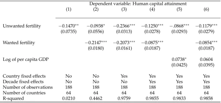
Table2reports coefficients of regression of human capital attainment, measured by the average years of schooling of the total population aged 25 and over, on unwanted fertility for different specifications and controls. In all regressions there exists a significant negative relationship between the fertility gap and educational attainment across countries. That is, when fertility is closer to its desired level, educational attainment is higher. This cor-relation is negative and significant even after including country fixed effects, and decade dummies, and controlling for per capita income and wanted fertility. Fertility behavior (unwanted and wanted fertility) explains about 44 percent of the variation in education
once in the sample.
17The sample period in our regression is different from his since we have access to more recent
Table 2: Relationship between human capital attainment and fertility (unwanted and wanted).
Dependent variable: Human capital attainment
(1) (2) (3) (4) (5) (6)
Unwanted fertility −0.1470∗∗ −0.0938∗ −0.2366∗∗∗ −0.1250∗∗∗ −.0868∗∗∗ −0.1179∗∗∗
(0.0735) (0.0556) (0.0313) (0.0278) (0.0293) (0.0279) Wanted fertility −0.2147∗∗∗ −0.2073∗∗∗ −0.0875∗∗∗ −0.0854∗∗∗
(0.0180) (0.0161) (0.0187) (0.0187) Log of per capita GDP 0.0738∗ 0.0604
(0.0425) (0.0395) Country fixed effects No No Yes Yes Yes Yes Decade fixed effects No No No Yes Yes Yes Number of observations 188 188 188 188 188 188 Number of countries 64 64 64 64 64 64 R-squared 0.0210 0.4462 0.9759 0.9855 0.9833 0.9858
Notes: Standard errors are in parentheses. The symbols∗,∗∗, and∗∗∗imply that coefficients are statistically
different from zero at 90, 95, and 99 percent confidence levels, respectively.
attainment in the sample, visible in Column (2). Educational attainment is also negatively correlated with wanted fertility, which reflects the quantity-quality trade-off.
Therefore what the reduced form evidence shows is a positive relationship between contraception use and education, via the reduction in the gap between actual and wanted fertility levels. Hence, the first question of this paper is: How much of the observed dif-ferences in education and income per capita can be explained by observed difdif-ferences in contraception use and fertility outcomes? And second, what are the aggregate effects of family planning interventions on development and inequality? In order to address these questions, we present an equilibrium model of economic development in which the con-trol of family size is costly.
3
Fixing Ideas
3.1
Demographics and endowments
with skills that they acquire during their childhood. They make the relevant economic de-cisions, including investment decisions. Old adults do not work and simply consume their savings. The production sector is characterized by a standard constant returns to scale technology, which depends on capital and efficiency units of labor.
3.2
Production
The consumption good is produced with a Constant Returns to Scale (CRS) technology that uses capital, K, and efficiency units of labor, L, as inputs. The technology is repre-sented by:18
Y= AKαL1−α, α ∈ (0, 1), A>0. (1)
Capital depreciates fully after use.
Let w be the wage rate and let R be the rental price of capital. Profit maximization implies that input prices are paid according to their marginal productivity, such that:
w = (1−α)AKαL−α, (2)
R = αAKα−1L1−α. (3)
3.3
Households
Fertility: Couples can have up to N > 0 children, and they can control their family size,
n, by investing in contraceptive use, such that:
n= N−θq, θ >0, (4)
whereq ≥0 is the (intensity of) investment in contraception (e.g., the use of pills or/and condoms) andθis related to the efficiency of contraception on birth control. Contraception is costly and the relative price of contraception isφq ≥0.
Human capital: Parents invest in the education of their children, e ≥ 0, such that the human capital of their children is given by
h′ =h(e) = eζ, ζ ∈ (0, 1). (5)
Investment in education is in terms of the consumption good. Children are also time consuming. Each child takes a fraction χ ∈ (0, 1) of her parents’ time endowment. We assume that parents are able to provide some hours in the labor market even when they have the maximum amount of children, i.e.,χN <1.
Preferences and optimal decisions:Consumption of couples during the young adulthood
period is denoted by cy, whilec′o denotes consumption of the couple in the next period,
when old. Preferences of households are represented by:
U(cy,c′o,n,h′) =log(cy) +βlog(c′o) +γlog(n) +ξlog(h′), (6)
18In order to simplify the notation we will abstract from the subscripttto denote the time period and use
whereβ,γ, andξare positive numbers.
Let s denote savings during the young adulthood period. The problem of the couple is to choosecy, c′o, q, s, ande to maximize (6) subject to (4), (5), and the following budget
constraints:
cy+s+φqq+en =wh(1−χn), (7)
c′o =R′s. (8)
Equation (7) states that consumption plus savings and expenditures on contraception and education equals income. Equation (8) implies that old couples consume their savings from the young adulthood period. Whenever q > 0, then the equations which describe
the solution of this problem are:19
cy = (1+1
β+γ)
wh−φq
θ N
, (9)
s = β
(1+β+γ)
wh−φq
θ N
, andc′o =R′s, (10)
e= ξζ (γ−ξζ)
whχ−φq
θ
, (11)
q = N
θ −
(γ−ξζ)
θ(1+β+γ)
wh−φq θ N whχ−φqθ
!
, (12)
n= (γ−ξζ) (1+β+γ)
wh−φq θ N whχ−φqθ
!
. (13)
We make the following assumption:
Assumption 1:Let Nχ<1 and (γ−ξζ)
(1+β+γ)χ < N.
The assumption thatNχ<1 implies that even when fertility is at its maximum (q =0),
couples still supply a positive number of hours to the labor market. The second part of the assumption implies that when the price of modern contraceptive methods is zero (φq = 0), then fertility is lower than the case in which there is no investment in modern
contraceptive methods (q = 0). Observe that when φq goes to zero then fertility does
not depend on labor income (wh). This is because when income rises the opportunity cost (time cost) of having more children rises (substitution effect), but since children are a normal good, then the income effect induces parents to have more children. With log-utility these two effects cancel each other out, and when φq = 0 then fertility does not
depend on income – see Equation (13). This is well explained inJones, Schoonbroodt, and Tertilt(2010). Whenφqis positive then there is a negative association between fertility and
income, as reported in the data. In this case richer parents can increase the intensity of
19Whenq=0, we have thatn=N,c
their use of contraceptive methods in order to control family size. Without investment in modern contraceptive methods, fertility is equal to N.
One can argue that it is not necessary to explicitly add investment in contraceptives into a standard quantity-quality fertility model because parameterχ, which corresponds to the time cost of children, could capture that investment. Better access to contraceptives could be translated into a rise in parameterχsuch that it would raise the quality of
chil-dren (e) as well as reduce their quantity (n). In fact, the proportional changes in n and e due to a proportional variation inχhave opposite signs but equal magnitude. A fall in the
price of contraceptives (φq) generates not only different quantitative but also qualitative
effects. Indeed, a fall in φq also increases e and reduces n, but observe that parameterχ
does not affect the consumption-saving decision, while the price of contraceptives does. In addition, family planning interventions which reduce the price of contraceptives have strong effects on the quantity and quality of children when income levels are low. Propo-sition1summarizes these findings.
Proposition 1. Let Assumption 1 be satisfied and defineǫz,χandǫz,φq as the elasticity of variable z∈ {n,e}with respect toχandφq, respectively. Then whenever q>0, we have that:
(i) ∂χ∂e >0, ∂n
∂χ <0and ∂χ∂s =0. Moreover, rχ =
|ǫn,χ|
ǫe,χ =1.
(ii) ∂φq∂e <0, ∂n
∂φq >0and ∂φq∂s <0. Moreover, rφq = ǫn,φq
|ǫe,φq| =
wh(1−Nχ)
wh−φθqN and
∂rφq ∂(wh) <0.
Proof. For the partial derivative, simply use equations (10), (11), and (13) and take the corresponding partial derivatives with respect to χ and φq. For the elasticities, take the
logarithm on both sides of equations (11) and (13) and differentiate either with respect to
χandφq. Q.E.D.
LetPdenote the number of young adult households such thatP′ =nP. In equilibrium, demand equals supply in all markets. In the labor market this means thatL =P(1−χn)h, and in the capital market, K′ = Ps. Let k denote physical capital per young household. In equilibrium with q > 0 it can be shown that h′ = Dk′ζ with D =
ξζ β
ζ
> 0, and
w(k) = (1−α)D−αAkα(1−ζ)(1−χn(k))−α. Whenq =0, we also have thath′ = Dk′ζ, and w(k) = (1−α)D−α(1−χN)−αkα(1−ζ). In addition,
n(k) = min
(
N, (γ−ξζ) (1+β+γ)
(1−α)D−αAkα+ζ(1−α)(1−χn(k))−α−φqθ N (1−α)D−αAkα+ζ(1−α)(1−χn(k))−αχ− φq
θ
!)
. (14)
Then the following proposition summarizes the fertility choice.
Proposition 2. Let Assumption 1 be satisfied. Then it can be shown that n(k) ∈ (1(+γ−β+ξζγ))χ,Ni and
(i) there exists a k(φq) > 0 such that if k ≤ k(φq), then n(k) = N; and if k > k(φq), then
(ii) for k >k(φq)fertility is decreasing with capital accumulation, i.e., n′(k)<0.
Proof. LetNχ <1. Then it can be shown that whenevern(k) <N, we have that
n′(k) =−
(γ−ξζ)
(1+β+γ)(α+ζ(1−α))(1−α)D−αAkα+ζ(1−α)−1(1−χn(k))−α φ q
θ (1−χN) 1+(1(+γ−βξζ+γ))α(1−α)D−αAkα+ζ(1−α)(1−χn(k))−α−1φq
θ (1−χN)
<0.
In addition, limk→∞n(k) = (1(+γ−β+ξζγ))χ. Equation (14) defines a critical value
k(φq) =
Nφq(1+β+ξζ)(1−χN)α
θ(1−α)D−αA((1+β+γ)Nχ−(γ−ξζ))
α+ζ(11−α)
, (15)
which is positive by assumption. Moreover, we have thatn(k) = Nfor anyk ≤k(φq)and
n(k) < N for anyk > k(φq). In order to see this, observe that without the upper bound
in the fertility choice,n(k)would go to infinity askwould be sufficiently small such that n(k)χwould tend to 1. Therefore, given the continuity ofn(k), we have that there exists a k(φq) >0 such thatn(k(φ)) = N. Using the Implicit Function Theorem we can show that
k′(φq) >0. Q.E.D.
The condition that equilibrates the capital market implies that
k′ =G(k;φq) =
β(1−α)D−αA(1−χN)−αkα+ζ(1−α)
(1+β+γζ)N fork≤k(φq),
β(1−α)D−αAkα+ζ(1−α)(1−χn(k))−αχ−φq
θ
γ−ξζ fork>k(φq).
(16)
Finally, we have that
h′ =Dk′ζ, (17)
and therefore human and physical capital are positively related.
We can now prove the following about the system of equations given by (14)–(17):
Proposition 3. (Existence and uniqueness of equilibrium path) For a given initial capital stock k0, let h0 be given by (17); then the dynamic system of difference equations (14)–(17) has a
unique trajectory (solution).
Proof. Givenk0and the fact thath0is given by (17), we can use (14) to findn(k0), which is unique given thatn(k)is non-increasing and continuous ink. Then, we can use Equations (16) and (17) to findk1(k0)and h1(k0), respectively; and so on. Q.E.D.
Given the path for nt, kt, and ht, we can find consumption and investment decisions
(9)–(11), as well as investment in contraceptive methods, Equation (12). Asymptotically, the system may diverge to infinity, converge to a zero, or converge to a non-zero steady-state equilibrium. Observe that when k < k(φq), we have that ∂G(k;φq)
∂k > 0,
andlimk→0∂G(∂kk;φq) =∞. Therefore, the system does not converge to a zero steady-state. If
k(φq)is sufficiently large,20 then there will be a locally stable steady-statek∗N = G(k∗N;φq)
in whichn(k) = N. In this case, there is no investment in modern contraceptive methods (q =0), and therefore family planning interventions do not have any effect on the long-run level of the capital stock, i.e,k∗Nis independent ofφq. However, wheneverk(φq) <k∗N, then
it can be shown that there exists a locally stable steady-state equilibriumk∗(φq) > k(φq)
such that fertility decreases with capital accumulation, and family planning interventions have long-run effects on capital accumulation and output. This is summarized in the following proposition.
Proposition 4. Let Assumption 1 be satisfied andφqbe sufficiently small such that k(φq) < k∗N.
Then there exists at least one locally stable steady-state equilibrium for capital per young household, k∗(φq) = G(k∗(φq);φq), such that in the neighbourhood of k∗(φq), fertility decreases with capital
accumulation, and family interventions which reduce the price of modern contraceptive methods increase the steady-state level of capital, i.e., k∗′(φq)<0.
Proof. If k(φq) < k∗N, then for any k > k(φq) it can be shown that ∂G(∂kk,φq) > 0, and
limk→∞ ∂G
(k,φq)
∂k = 0. This implies that k′ = G(k,φq) has to cross (at least once) the 45
degree line (k′ = k) from above, and this defines k∗(φq) = G(k∗(φq);φq), which is
there-fore locally stable. Fertility thus decreases with capital accumulation. Moreover, we can easily show thatk∗′(φq) <0, which completes the proof. Q.E.D.
Corollary 1. Let Assumption 1 be satisfied; then human capital increases with physical capital accumulation. If φq is sufficiently small such that k(φq) < k∗N, then family interventions which
reduce the price of modern contraceptive methods increase the steady-state level of human capital.
Proof. This follows directly from Equation (17) and Proposition4. Q.E.D.
Therefore, the above model is able to replicate the negative relationship between fer-tility and income through the intensity of the use of modern contraceptive methods. The model shows that the standard fertility model without the decision to invest in contra-ceptives cannot capture how family planning interventions affect the quantity and quality of children, as well as savings. This framework, however, corresponds to the simplified version of the model. Here agents are homogeneous, there is no uncertainty in the fertil-ity decision, and households cannot rely on abortion to control family size. In addition, given prices, there are no unwanted births in the model. We believe that introducing such features is important in accurately assessing the effects of family planning interventions on fertility decisions, investment, inequality, and output. For instance, the homogenous nature of the framework prevents us from studying how reductions in the price of mod-ern contraceptive methods affect the fertility decisions of different families, and how such reductions can affect the persistence of inequality in education and income. Below we de-scribe a more elaborate version of our theoretical framework which we use for our quan-titative analysis.
4
Model
4.1
Demographics and Endowments
Here we keep the environment as close as possible to the one presented in the previous sec-tion. As before, the economy consists of overlapping generations of individuals who live for three periods: childhood, young adulthood, and old adulthood. Children do not make any economic decisions and can acquire skills. Young adults are organized as couples and make the following economic choices: their desired number of children and the intensity of their contraceptive use. The number of pregnancies is, however, stochastic, and the re-alized and desired number of pregnancies may be different. The use of contraception can lower the chances of an unwanted pregnancy. Once the number of pregnancies is realized, young couples may decide to abort some of them to close the gap between the number of realized and desired children. But abortion is costly, both in terms of utility and in income. Young adults have one unit of productive time and are endowed with skills that they ac-quired during their childhood. They then invest their income into the education of their children, consume, and save. Old adults do not work and simply consume their savings.
The production side of the model is similar to the one presented in Subsection3.2with firms’ optimal conditions given by (2) and (3).
4.2
Households
Desired and realized fertility: Young couples first decide on the number of children that
they want to have, ˜n.21 Then, the number of pregnancies,p, is realized. We assume that
p−n˜ =max{η−θq, 0}, (18)
where q ≥ is the investment in contraception, η is a random variable with distribution
Γ(η)and support[0,N], andθis a positive parameter.22 It is important to emphasize that
even when modern contraceptive use is zero (q = 0) pregnancies will still have a deter-ministic (demand) component, ˜n, and a stochastic component,η. We are not saying that without modern contraceptive methods families could not use traditional practices to con-trol fertility (e.g., extended breast-feeding and sexual abstinence, among others). Equation (18) simply implies that the use of modern contraceptive methods can decrease the fertility gap relative to a situation without these birth control (supply) technologies. Contraceptive prevalence (or use) is jointly determined by both supply and demand factors and therefore is able to disentangle the importance of each factor in the determination of fertility.
21Since adults are organized as couples, we can view ˜nas the desired number of children that each
house-hold wants to have. We abstract from intra-househouse-hold bargaining over fertility. Doepke and Kindermann
(2016) explore in detail the consequences of bargaining over fertility for a set of European countries.
22We could easily assume that instead of Equation (18), we have thatp−n˜ = η−θq. Then households
Contraception is costly and the relative price of contraception is φq. This includes not
only the price to buy modern contraceptives on pharmacies or to acquire (including trans-portation costs) them in public clinics, but also the fact that they might be stocked out, as reported byAshraf, Field, and Lee(2014) in the case of Zambia. Therefore,φqcorresponds
to supply factors which might affect the use of modern contraceptive methods. Contra-ception also generates a utility cost Ψq > 0 wheneverq > 0. In some cultures, modern
contraception use can be associated with promiscuity and women may also have the fear of side effects and adverse reactions related to, for instance, the use of pills. In addition, there may potentially be intra-household disagreement (husband versus wife desired fer-tility), which is not explicitly modelled here, about the use of contraceptives. For instance,
Ashraf, Field, and Lee(2014) show that when women receive access to contraception alone they report lower subjective well-being than when they receive access to contraception with their husbands, suggesting a psychosocial cost.23 Therefore, the parameter Ψq > 0
corresponds to demand barriers to the use of modern contraceptive methods. Once the number of pregnancies is realized, the household can choose to abort some of them,a, in order to close the gap between the number of realized pregnancies and the desired num-ber of children. Abortion is costly both in terms of utility, such that there are disutility costsΨa >0 whenevera>0, and in terms of the consumption good. The relative price of
abortion isφa. The realized number of children is:
n = p−a. (19)
Observe that while investment in the use of modern contraceptives is an insurance against the risk of unwanted pregnancies, abortion is not an insurance since it terminates a preg-nancy with certainty. However, both technologies incur costs and agents will take this into account when making their birth control choices.
Human capital: Parents invest in the education of their children, e ≥ 0, such that the human capital of their children is equal to
h′ =ǫh(e)˜ . (20)
The function ˜h(e)is increasing, differentiable, and concave with respect toe, and the price of education in terms of the consumption good is λ(e), which varies with e. We also as-sume that ˜h(0) > 0 such that the quality of children’s income elasticity is increasing with
income, as postulated byBecker(1960) and explored by Greenwood, Seshadri, and Van-denbroucke(2005), to generate the secular decline in fertility and the increase in human capital. The shock ǫ ∼ F(ǫ) has positive support and summarizes unobserved factors that influence the human capital production process. Investment in education is in terms of the consumption good. Children are also time consuming. Each child takes a fraction
χ∈ (0, 1)of her parents time endowment andNχ<1.
23We are abstracting from externalities when fertility desires are influenced by the reproductive behavior
Optimal decisions: Consumption of couples during the young adulthood period and old adulthood period are denoted bycyand c′o, respectively. Preferences of couples are
repre-sented by the following utility function:
U(cy,c′o,n,h′), (21)
whereU(·,·,·,·)is differentiable, increasing, and concave in all arguments.
Let s be the savings of a young adult couple andIa>0 be an indicator function which
equals one when a > 0 and zero otherwise. The problem of the couple with p realized
pregnancies who investedqin contraception is to choosecy, c′o, a,s, andeto maximize
˜
V(h,p,q) = max
cy,c′o,a,s,e≥0
{Eǫ[U(cy,c′o,n,ǫh(e))]˜ −ΨaIa>0}, (22)
subject to (19) and (20),
cy+s+φqq+φaa+λ(e)en =wh(1−χn), (23)
c′o =R′s. (24)
Eǫ[·] corresponds to expectations over ǫ. Equation (23) corresponds to the budget con-straint of the young couple. It implies that consumption plus savings of the household plus expenditures on contraception, abortion, and education must be equal to income. Budget constraint (24) states that in old adulthood, couples consume the principal and interest from their savings during the young adulthood period.
LetIq>0be an indicator function which equals one whenq >0 and zero otherwise. The
problem of a couple before the number of pregnancies is realized is to choose the number of desired children, ˜n, and investment in contraception,q, in order to:
V(h) = max ˜
n,q≥0{Eη[V(h˜ ,b,q)−ΨqIq>0]}, (25) subject to Equation (18). The notation Eη[·] denotes that expectations are taken over the stochastic number of pregnancies summarized by the random variableη.
4.3
Equilibrium
In a competitive equilibrium, agents and firms optimally solve their problems and all mar-kets clear. Letx = (h,η)withx ∈ X = (0,∞)×(0,N). The couples’ optimal behavior
de-fines optimal policy functionscy(x), c′o(x),s(x),q(h),a(x),e(x), and ˜n(h). The stationary
equilibrium in this economy is characterized by a stationary human capital distribution associated with the optimal behavior of couples and firms. To characterize the stationary human capital distribution, first define the following function,
1(x,ǫ,h′) =
(
The function above takes the value of one if a child coming from parents with a state x and a shockǫbuilds a human capital level h′ . It takes the value of zero otherwise. Next, construct a transition probability function,
P(h′|x) =
ˆ
1(x,ǫ,h′)dF(ǫ),
which computes the probability that a child attains human capital levelh′conditional on having parents with state x. Finally, note that the number of children of a household is given by
n(x) = n(h) +˜ max{η−θq(h), 0} −a(x). Based on this, define the distribution function of human capital as
Υ(h′) = ´
X n(x)P(h′|x)dΥ(h)dΓ(η)
´
X n(x)dΥ(h)dΓ(η)
. (26)
The distribution of human capital in the economy isΥ. The rate of population growth, g,
in this economy is given by
1+g=
ˆ
X n(x)d
Υ(h)dΓ(η). (27)
The law of motion for the distribution presented in Equation (26) takes into account pop-ulation growth as evidenced by the normalization in the denominator. Note that in this economy both capital and labor will grow with the rate of population growth. To pose a stationary representation of the equilibrium, one can de-trend these two variables in the following way,
L = Lt (1+g)t,
and
K = Kt (1+g)t.
Definition: (Stationary Competitive Equilibrium)A stationary competitive equilibrium for this economy consists of allocations for firms{K,L}, a collection of policy functions for households {cy(x),c′o(x),s(x),q(h),a(x),e(x), ˜n(h)}, a stationary distributionΥ, a vector of prices{w,R},
and a population growth rate g such that:
i. Given the vector of prices{w,R}, the vector{K,L}solves (2) and (3).
ii. Policy functions q(h)andn(h)˜ solve value function V(h)and
p−n(h) =˜ max{η−θq(h), 0}.
iii. Policy functions{cy(x),co′(x),s(x),a(x),e(x)}solve value function
˜
iv. Market clearing conditions are such that:
ˆ
X[cy(x) +s(x) +
φqq(x) +φaa(x) +λ(e)e(x)n(x)]dΥ(h)dΓ(η) (28)
+ 1
1+g
ˆ
X
co(x)dΥ(h)dΓ(η) = AKαL1−α,
L=
ˆ
X
h(1−n(x)χ)dΥ(h)dΓ(η). (29)
and
K′ =
ˆ
X
s(x)dΥ(h)dΓ(η). (30)
v. The distribution of human capitalΥsolves (26).
vi. The population growth rate is given by (27).
5
Fitting the Model to the Data
In order to investigate the effects of family planning interventions on human capital dy-namics, inequality, and income, we must assign values for the model parameters. We have prior information about some parameters, such as the capital share in income. Other pa-rameters are specific to the analysis at hand and little is known about their magnitudes. Therefore, values for these parameters will be estimated such that the model matches key micro and macro moments of Kenya for the late 2000s, due to data restrictions. We use a minimum distance procedure which targets a set of data moments on wanted and un-wanted fertility and family planning in terms of contraceptives and abortion conditional on education levels. These data moments are derived from the 2008 Kenya Demographic and Health Survey.24 Matching the cross-sectional distributions of fertility and family planning conditional on human capital ensures that the model delivers a credible link be-tween fertility uncertainty, family planning instruments to mitigate it, and human capital accumulation. We concentrate on the following levels of education: 0 years of schooling, 4 years of schooling, 8 years of schooling, 12 years of schooling, and 16 years of schooling. We also target several aggregate moments such as income inequality, the consumption-output ratio, and the capital-output ratio, among others. First, however, we need to impose func-tional forms for some of the expressions of our theoretical framework. Below we describe in detail these functions and how we calibrate and estimate model parameters.
5.1
Calibration and Estimation
Model period: The model period is assumed to be 20 years. This is consistent with the
2008–2014 average life-expectancy in Kenya of around 60 years (cf.,The World Bank,2015).
Production technology: Recall that we assumed a Cobb-Douglas production function. The capital share in income we get from the Penn World Tables (cf.,Feenstra, Inklaar, and Timmer, 2015). We set it to α = 0.36, which is consistent with the number estimated by
Gollin(2002) for developing countries. Capital depreciates fully after use. The produc-tivity parameter A is chosen such that total output per capita is normalized to 1. The production technology parameters are: Aandα =0.36 (one to be estimated).
Fertility technology: The fertility shockη has the following cumulative distribution func-tion:Γ(η) = η
N κ
, whereNcorresponds to the maximum number of unwanted pregnan-cies possible. We set the maximum number of unwanted pregnanpregnan-cies per woman to 10. In the grid for wanted fertility we also set the maximum number of wanted pregnancies to 10 so that a woman could have a maximum of 20 pregnancies in her lifetime. Since the model period is one year, this implies one pregnancy per year. The efficiency of contraception is determined by the product ofθq. Different combinations of parametersφq and θ lead to
identical choices of consumption and fertility. In order to resolve this issue, we normalize the price of contraception to one such thatφq = 1. The relative price of abortion is equal
toφa > 0. The fertility technology parameters are: N = 10, φq = 1, κ, θ, and φa (three to
be estimated).
Human capital function and child-rearing technology: The offsprings’ human capital
is given by h′ = ǫh(e)˜ . We assume that ˜h(e) = h0+h1eζ. The fixed component h0 im-plies non-homothetic preferences over human capital. This feature and the time cost of children, χ, help us generate a negative relationship between fertility and parental in-come/education in the model.25 We restrict the choice of education to five discrete op-tions: no education, four years, eight years, twelve years, and sixteen years. Each of these five discrete levels bears an education cost. The vector of education costs λ(e) ∈ {0,λ1,λ2,λ3,λ4} summarizes the amount of consumption goods parents need to forgo in order to finance the education of a child to one of these five attainment levels. The unobserved ability that augments the human capital production,ǫ, is assumed to have a log-normal distribution with mean 0 such that lnǫ ∼ N(0,σǫ2). There is also the time cost of raising a child,χ. The parameters for this section are: χ, h0,h1,ζ, λ1, λ2,λ3,λ4, andσǫ2 (nine to be estimated).
Utility: Turning to preferences, the utility function takes the following functional form:
U(cy,c′o,n, ˜h(e)) =log(cy) +βlog(c′o) +γlog(n) +ξlog(h(e))˜ .
There are also two costs related to the household’s taste: the disutility of contraception use and abortions. Recall that these were defined asΨqIq>0andΨaIa>0withΨq >0 andΨa >
0, whereIq>0andIa>0are indicator functions when the use of modern contraceptives and
abortion are positive, respectively. That is, households pay these costs if they engage in strictly positive use of each family planning option. Preference parameters are: β, γ,ξ,Ψq
andΨa(five to be estimated).
25SeeGreenwood, Seshadri, and Vandenbroucke(2005) andJones, Schoonbroodt, and Tertilt(2010) for
There are therefore 18 parameters of the model to be estimated via a minimum distance procedure. The parameters are estimated to match the normalization of output per capita to one and the following 23 data moments:
(i) Realized fertility rate and unwanted fertility rate by levels of education. Note that matching these two series implies that the level of wanted fertility is matched too. Source: 2008 Kenya DHS.26[8targets]
(ii) Abortion rates and the fraction of women using modern contraception by levels of education. Source: 2008 Kenya DHS and own calculation based onWestoff(2008).27 [8targets]
(iii) Fraction of people in each education category. Source: 2008 Kenya DHS. [4targets] (iv) Capital-output and consumption-output ratios. Source: Penn World Tables (cf.,
Feen-stra, Inklaar, and Timmer,2015) . [2targets]
(v) Gini coefficient of household labor income. Source:The World Bank(2015). [1target] How do these data moments aid in the process of setting the model parameters? In a gen-eral equilibrium setup a change in any parameter affects all targets. However, some sets of data moments are more sensitive to certain parameters. The fertility and family planning targets ((i) and (ii)) conditional on human capital are useful in recovering preference pa-rameters{γ,ζ,Ψq,Ψa}and the price of abortionφa, as well as the fertility uncertainty{κ},
the efficiency of modern contraceptives θ, and the time cost per child χ. The distribution over educational categories (iii) identifies the cost parameters{λ1,λ2,λ3,λ4}. The capital to output ratio helps to pin down the discount factor β. Matching aggregate targets (iv) along with targets on fertility, family planning, education, and inequality (v) help us in setting parameters for the human capital accumulation process{h0,h1,σǫ}.
Let Θ = {β,γ,ξ,Ψq,Ψa,h0,h1,ζ,χ,σǫ,κ,θ,φa,λ1,λ2,λ3,λ4,A} be the vector of
param-eters to be estimated, and define the difference between the model-generated 23 mo-ments and the normalization of output to one by M(Θ), and the data moments D by
R(Θ) = D − M(Θ). The minimum distance estimation amounts to choosing parameter
values that minimize the squared form, ˆ
Θ =argmin
Θ R(
Θ)′WR(Θ),
whereWis a diagonal weighting matrix. We use an identity matrix in our base estimation. Table3reports the calibrated and estimated parameter values that result from the baseline estimation procedure above for Kenya.
26In the model there are five levels of education: no schooling, 4 years of schooling, 8 years of schooling,
12 years of schooling, and 16 years of schooling. In the DHS survey there are four levels of education: No primary education, primary, secondary, and higher and more. Primary education in Kenya corresponds to 8 years of schooling. Therefore, in the map from the model to the data, we aggregate the no-education category and the 4-years-of-schooling category into one category, which corresponds to no primary education or from 0 to 4 years of schooling.
27The total abortion rate is calculated using Equation (7) ofWestoff(2008). This equation defines a
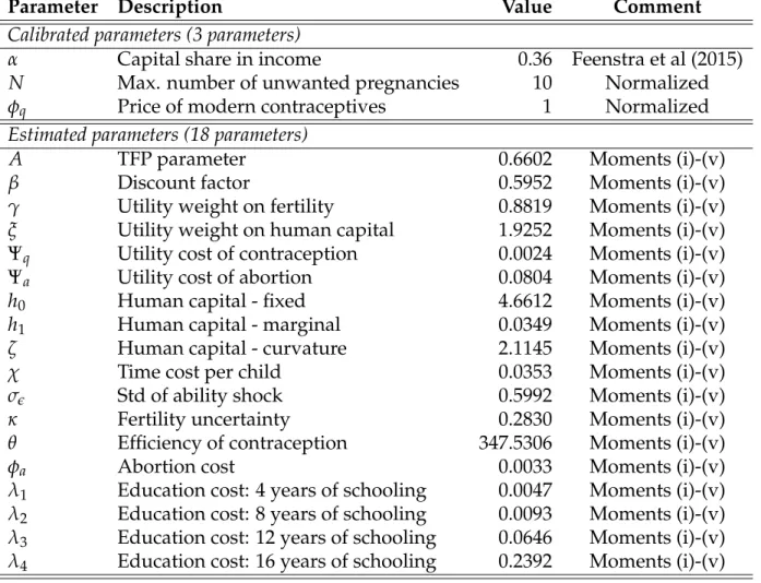
Table 3: Calibrated and estimated parameters
Parameter Description Value Comment
Calibrated parameters (3 parameters)
α Capital share in income 0.36 Feenstra et al (2015)
N Max. number of unwanted pregnancies 10 Normalized
φq Price of modern contraceptives 1 Normalized
Estimated parameters (18 parameters)
A TFP parameter 0.6602 Moments (i)-(v)
β Discount factor 0.5952 Moments (i)-(v)
γ Utility weight on fertility 0.8819 Moments (i)-(v)
ξ Utility weight on human capital 1.9252 Moments (i)-(v)
Ψq Utility cost of contraception 0.0024 Moments (i)-(v)
Ψa Utility cost of abortion 0.0804 Moments (i)-(v)
h0 Human capital - fixed 4.6612 Moments (i)-(v)
h1 Human capital - marginal 0.0349 Moments (i)-(v)
ζ Human capital - curvature 2.1145 Moments (i)-(v)
χ Time cost per child 0.0353 Moments (i)-(v)
σǫ Std of ability shock 0.5992 Moments (i)-(v)
κ Fertility uncertainty 0.2830 Moments (i)-(v)
θ Efficiency of contraception 347.5306 Moments (i)-(v)
φa Abortion cost 0.0033 Moments (i)-(v)
λ1 Education cost: 4 years of schooling 0.0047 Moments (i)-(v)
λ2 Education cost: 8 years of schooling 0.0093 Moments (i)-(v)
λ3 Education cost: 12 years of schooling 0.0646 Moments (i)-(v)
λ4 Education cost: 16 years of schooling 0.2392 Moments (i)-(v)
5.2
Model Fit
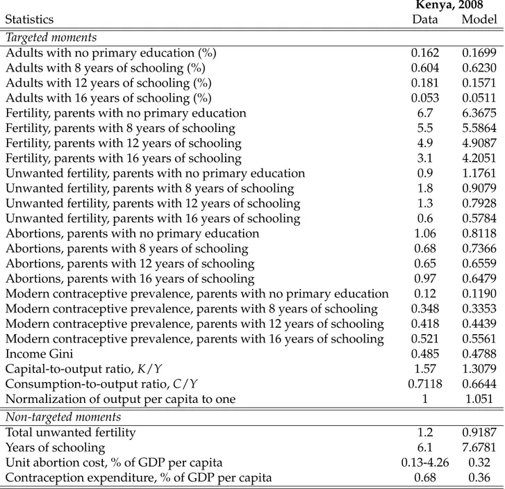
Now, we discuss the fit of the model with respect to targeted and some non-targeted mo-ments. We estimated a total of 18 parameters by targeting 23 data moments and setting the normalization of output per capita to one. Table4 reports these moments in the data and in the model.
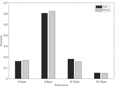
Figure 1: Data versus model - Fraction of adults by education. Source: 2008 Kenya DHS.
The model matches the fraction of adults in each education category very well, as seen in Figure1.28 The model does also a good job in reproducing the pattern of modern con-traceptives prevalence and the total fertility rate conditional on the level of human capital observed in the data.29 (See Figures2(a)and2(c).) Therefore, the model replicates qualita-tively and quantitaqualita-tively the trade-off between child quantity and quality which is present in the empirical evidence. The model does generate, however, a lower number of abortions than in the data for the lower tail and upper tail of the abortion distribution conditional on the level of education, but observed abortions in the middle of this distribution match well.30 (See Figure2(b).) Regarding unwanted fertility, the model overestimates by 30 per-cent this measure for adults with no primary education and underestimates by 50 perper-cent this measure for adults with a primary education degree. (See Figure2(d).) Since the frac-tion of adults with primary educafrac-tion is about 3.7 larger than the fracfrac-tion of adults with
28According toBarro and Lee(2013) the average amount of schooling for the adult population in Kenya is
6.1 years. The model counterpart is 7.68 years. If we calculate the average years of schooling using the DHS data this number is 7.83, which is very close to what is generated by the model.
29Only at the very top of the human capital distribution does the model miss the fertility rate by
underes-timating it.
30We could introduce some heterogeneity in the utility cost of abortion in order to exactly reproduce the