USING FAULT MODELS IN STATE OBSERVERS METHODOLOGY FOR CRACK DETECTION IN CONTINUOS SYSTEMS

(1)

Using Fault Models in State Observers Methodology for Crack Detection in Continuos SystemsRevista Sul-Americana de Engenharia Estrutural

http://dx.doi.org/2867/rsee.v13i1/573

Using Fault Models in State Observers

Methodology for Crack Detection in Continuos

Systems

Gilberto Pechoto de Melo1_{, Marco Anderson da Cruz Araujo}2_,

Edson Luiz Valverde Castilho Filho3_{, Lucas Rangel de Oliveira}4

ABSTRACT

Nowadays a major factor of interest in industries in relationship to development of new techniques for detection and localization of faults it is the concern with the secu-rity of their systems. There is need for supervising and monitoring in order to detect and correct any fault as fast as possible. It is verified actually, that some determined parameters of the systems may vary during the process, due to the specific characte-ristics or the natural wearing of its components. It is known that even in well-desig-ned systems the occurrence of cracks in some components can cause economic losses or lead to dangerous situations. With the help of the state observers methodology one can reconstruct the unmeasured states of the system, since that it is observable, becoming possible in this way to estimate the measures for locations of difficult ac-cess. The technique of state observers consists in developing a model for the system under analysis and comparing the estimate of outcome with the measured one, the difference between these two resulting in a residue that is used for analysis. In this work a bank of signals associated to a model of crack was assembled in order to follow its progress. The data acquired from the computational simulations in a cantilever beam discretized by means of the technique of finite elements, had been sufficiently satisfactory, validating the proposed methodology.

Keywords: State Observers, faults detection and location, crack model, finite element.

1_{Prof. Adjunto do Dep. Eng. Mecânica - UNESP/Faculdade de Engenharia de Ilha Solteira. Av. Brasil Centro, 56}

CEP. 15385-000. Ilha Solteira, S.P – Brasil. Telefone: (18) 3743-1052. E-mail: [email protected]

2_{Mestre em Eng. Mecânica - UNESP/Faculdade de Engenharia de Ilha Solteira. Av. Brasil Centro, 56 CEP.}

15385-000. Ilha Solteira, S.P – Brasil. (18) 3743-1052.E-mail: [email protected]

3_{Mestre em Eng. Mecânica - UNESP/Faculdade de Engenharia de Ilha Solteira. Av. Brasil Centro, 56 CEP.}

15385-000. Ilha Solteira, S.P – Brasil. (18) 3743-1052. E-mail: [email protected]

4_{Aluno de Doutorado em Eng. Mecânica - UNESP/Faculdade de Eng. Ilha Solteira. Av. Brasil Centro, 56 CEP.}

(2)

Revista Sul-Americana de Engenharia Estrutural, Passo Fundo, v. 13, n. 2, p. 7-25, maio/ago. 2016

8

1 Introduction

The increasing technological advances verified during the last decades demand from the machines and mechanical structures, each time more, larger capacities of producing work under speed of operation moreover, currently one of the biggest con-cerns of the industry is how to keep equipment operating all the time avoiding sudden faulty stops, which explains the constant development of new techniques of detection and location of faults in mechanical systems submitted the dynamics efforts. With the purpose of assuring the operation of the mechanical systems with safety, these should be supervised and as well as monitored for the flaws to be identified following their progress scheduling a maintenance program for the most appropriate moment, since inherent disturbances to the operation of these systems can lead to a deterioration of the system performance or even to severity dangerous situations.

The state observer's technique consists on a method capable of reconstructing the states in cases for which their measurement becomes difficult or even impossible. This way, flaws can be detected in those points even without the knowledge of their measu-rements, could also monitor them through those reconstructions of your states. On the other hand, this technique consists on developing a model for the system under analy-sis and comparing the output for the observer with the one of the system.

Once identified the flaws the challenge moves on to monitoring the form system in order to analyze the reliability and the compromising level caused by each identified flaw. It is known that the occurrence of cracks in some components can take to not planned stops causing financial damages or even dangerous situations. This analysis allows to accompany the propagation of the same and through some pre-defined crite-ria and to program the maintenance in the system for the most appropcrite-riate moment.

The main focus of the literature revision has been the detection and location of mechanical system faults. Theories which are related to state observers and crack mo-deling have been taken in its account. The state of the art is presented in chronological order and the most significative works are selected.

Luenberger (1964). Luenberger states that the major part of the theory of

mo-dern control is based on the assumption that the state vector of the system to be con-trolled is available fro direct measurement. However, in many practical situations, just few of output database available. The author shows how the inputs and outputs that are available can be used to build an estimate observer, or just observer. This work states the state observer theory.

Luenberger (1966). Has shown that for a linear system, its state vector can be

approximately reconstructed by means of an observer designed. The “n” order state vector with “m” independent outputs can be reconstructed, rebuilding the remaining states from differential conditions. He proved also that the design of observer with “m” outputs can be reduced a design “m” observer as if they were simple output subsystems simplifying the observer complexity.

(3)

Using Fault Models in State Observers Methodology for Crack Detection in Continuos Systems

Watanabe and Himmelbleau (1982). The authors have presented a method to

detect instruments faults in nonlinear time dependent processes, including uncertain-ties such as modeling mistakes, parameters ambiguity and input and output noise. The main goal of their work has been the development of state estimate filters with minimum sensitivity to uncertainties and maximum sensitivity to instruments faults, like those corresponding to slight deterioration or gradual chances, instead or sudden or catastrophic faults. The authors have employed the concept of robust observer, intro-duced by Clark (1978), with designing state estimation filters for instruments default detection, robust enough to with stand the uncertainties. The base for the filters was the separation of the effects of faults from the uncertainties.

Yuen, M. M. F. (1985). He has considered damaged cantilever beam in the

wi-tch the damaged location dimensions were unknowing. The modeling of the stiffness change has been simulated by a reduction on the elasticity modulus of the section. In the way, the damaged extension can be related to the reduction degree. They have proposed a new idea of defect insulation by means of robust observation, from which a defect diagnosis law is found in such away to monitor the components of a system and a diagnosis system is design following a systematic procedure. The results from that technique have shown that robust approach for defective components coupled by unavailable states can be effectively detected.

Ge, W. and Fang, C. Z. (1988). The authors have described a novel conception for

the detection of components under failure by robust observation. Considering a ma-thematical model corresponding to “m” components coupled by non-estimated states. They have determined the design of devices to monitor the operation of those “n” com-ponents and faults detection. In the case an observable system, some first or superior order components can be monitored for the purpose of diagnosis without information of possible faults modes. Due to the observer robustness, the authors have analyzed some reactions such as linearization and measurement errors, noise presence, numerical errors, and so on.

Qian (1990). He has established the elements stiffness matrix and motion

equa-tion for a cracked beam. According to the Saint Venant principle, the tension field is disturbed in a region close to the crack only. The whole element stiffness matrix, with exception to the cracked element, remains unaffected, obeying to certain constraints in the element size. The energy of the crack is additional tension is evaluated from frac-ture mechanics theory and the flexibility coefficient in expressed by an intensity factor derived from the Castigliano Theorem, on linear elastic field.

Choy et al. (1995). He has presented a methodology based on the vibration theory

that can be used for faults detection in finite element modeling systems, employing beam elements supported by an elastic foundation. The identification and localization of a fault on the beam are obtained by “m…” a change in the Young´s modulus for that particular beam element. Assuming that for the original system the Young´s modu-lus is well-know the natural frequencies of the system are numerically evaluated by

(4)

10

means of suitable mathematical model, experimentally validated in a crack develops on a certain beam element. There is an alteration in the system natural frequencies, considering just one faulty element, the procedure starts up supposing that the crack is located on the first elements. The corresponding Young´s modulus is adjusted until the first natural frequency matches the measured one. The process is repeated for each element.

Melo, G. P. (1998). He has developed a methodology for the detection and

loca-lization of faults in mechanical system employing reduced order state observers. He has shown the way non measured states can be reconstructed. By “means” of robust state observers, he could provide localization of faults, with the help of several robust state observer data bank, for each system parameter, he has proved that it is possible to quantify the system faults. He has preserved computing simulations and laboratory experiments “validating” the theory.

Cacciola, P., Muscolino, G. (2002). They have employed a cantilever beam,

fi-nite element “discretized“ for a crack closing model, considering completely open or closed cracks, in order to describe the damaged element. Once defined the beam mathe-matical model, the dynamical outcome is evaluated, applying a numerical procedure, based on the fundamentals of dynamical changing structural systems. To the stochas-tic case, the enhanced perturbation method is modified in order to efficiently solve the nonlinear stochastic differential equations.

Muscolino G. et al. (2003). They have used vibration analysis of a cracked beam,

by means of stochastic analysis to detect the presence and localization of has been employed in order to apply the Monte Carlo method to evaluate in the domain, the statistical high order of the nonlinearities.

Lemos (2006). He has presented the state observer methodology for detection and

location of faults in rotary systems, taking into account their foundations. According to him, the state observer methodology is able to reconstruct non measured states or esti-mate values coming from difficult access locations in the system. On fact, those faults can be detected without the need for a direct measurement.

Zacarias (2008). In this work was set up a bank of observers associated to a

mo-del of crack in order to follow its progress. The results gotten through computational simulations in a cantilever plate discretized by using the finite elements technique and the accomplished experimental analysis were sufficiently satisfactory, validating the developed methodology.

Fault detection technique employing state observers can reconstruct non measu-red states or values of difficult access locations. In that case, faults can be detected and monitored without measurements. The technique consists on developing a system model and comparing the estimated output with the measured one. The main idea is to use a crack model to build an observer bank, capable of supervising the process in which each observer is dedicated to an amount of deep of the crack. Actually a cracked

(5)

beam when submitted in an alternate effort or to an initial condition, causes openings and closings alternately. However, when the crack remains closed, the stiffness does not change. In the present work, for fault diagnosis, only the case of opening crack has been considered.

2 Analytical model of the cracked beam

The presence of a crack in the beam, according to the principle of Saint Venant, causes a perturbation of the stress field in the neighborhood of the breach. Such a per-turbation is relevant specially when the crack is open and determines a local reduction of the flexural stiffness. On the other hand, when the crack is closed the beam acts, approximately, as a homogeneous beam with no crack. According to author Muscolino the stiffness matrix is the structural property that is most affected from the breathing of the crack, as damping and mass matrices do not change appreciably during the ope-ning and closure of the crack.

Undamaged elements of the beam are modeled by Euler type finite elements with two degrees of freedom (transverse displacement and rotation) at each node. The cra-cked element will be modeled as an undamaged element if the crack is closed whereas it exhibits a more flexible behavior if it is open.

2.1 Stiffness matrix

The strain energy of an element without a crack, neglecting shear action, can be written as

(1)

Where E is the Young modulus, I the moment of inertia, l the length of the finite element. P and M are shear and bending action, respectively, synthesizing the presence of the elements situated at the right of the element, while the behavior of the elements situated at the left of the finite element are considered as constraints. The calculation of the additional stress energy of a crack has been studied in fracture mechanics and the flexibility coefficients are expressed by a stress intensity factor in the linear elastic ran-ge using Castigliano’s theorem. The additional energy, in the case of a rectangular beam of height h and width b, due to the crack can be written as (Cacciola P., Muscolino G.):

∫

+ + + = a I II III _da E K E K K b W 0 2 2 2 ) 1 ( (1 ) '

ν

₍₂₎

(6)

12

where E’=E for plane stress, E’=E/(1+ν) for plane strain and a is the crack depth. Taking into account only bending, Eq. (2) leads to

∫

+ + = a IM IP IIP _da E K K K b W 0 2 2 ) 1 ( ' ) ( ₍₃₎ Where Where ); ( 6 2 aF s bh M KIM I ( ); 3 2 aF s bh Pl KIP I aF (s) bh P KIIP II (4)

are stress intensity factors for opening-type and sliding-type cracks due to M and P, respectively, and 2 cos 2 1 199 . 0 923 . 0 2 2 ) ( 4 s s sen s tg s s FI s s s s s s s F_II 1 18 . 0 085 . 0 561 . 0 122 . 1 ) 2 3 ( ) ( 2 2 3 ₍₅₎

Being s the ratio between the crack depth and the height of the element (s = a/h). The elements of the compliance (or flexibility) matrix ce(0) of the undamaged element can be

derived as M P P P j i P P W c j i o o ij 1 2 ) ( 2 ) ( _; _, ₁_,₂_, _, ₍₆₎

And the elements of the additional flexibility ce(1) matrix are

M P P P j i P P W c j i ij 1 2 ) 1 ( 2 ) 1 ( _; _, ₁_,₂_, _, ₍₇₎

Finally the total flexibility matrix for the element with an open crack is

) 1 ( ) 0 ( e e e c c c (8)

From the equilibrium conditions, the following relationship holds

T i i T i i i i M P M T P M P 1 1 1 1 (9) With T l T 1 0 1 0 0 1 1 (10)

From the principle of virtual work the stiffness matrices of the undamaged and cracked element can be respectively written as

T e u Tc T k (0)1 T e c Tc T k 1 ₍₁₁₎ (4) are stress intensity factors for opening-type and sliding-type cracks due to M and P, respectively, and Where ); ( 6 2 aF s bh M KIM I ( ); 3 2 aF s bh Pl KIP I aF (s) bh P KIIP II (4)

are stress intensity factors for opening-type and sliding-type cracks due to M and P, respectively, and 2 cos 2 1 199 . 0 923 . 0 2 2 ) ( 4 s s sen s tg s s FI s s s s s s s FII 1 18 . 0 085 . 0 561 . 0 122 . 1 ) 2 3 ( ) ( 2 2 3 ₍₅₎

Being s the ratio between the crack depth and the height of the element (s = a/h). The elements of the compliance (or flexibility) matrix ce(0) of the undamaged element can be

derived as M P P P j i P P W c j i o o ij 1 2 ) ( 2 ) ( _; _, ₁_,₂_, _, ₍₆₎

And the elements of the additional flexibility ce(1) matrix are

M P P P j i P P W c j i ij 1 2 ) 1 ( 2 ) 1 ( _; _, ₁_,₂_, _, ₍₇₎

Finally the total flexibility matrix for the element with an open crack is

) 1 ( ) 0 ( e e e c c c (8)

From the equilibrium conditions, the following relationship holds T i i T i i i i M P M T P M P 1 1 1 1 (9) With T l T 1 0 1 0 0 1 1 (10)

T e u Tc T k (0)1 T e c Tc T k 1 ₍₁₁₎ (5)

Being s the ratio between the crack depth and the height of the element (s = a/h).

The elements of the compliance (or flexibility) matrix c_e(0)_{of the undamaged element}

can be derived as

Where

); ( 6 2 aF s bh M KIM I

(

);

3

2

a

F

s

bh

Pl

K

IP I

aF (s) bh P KIIP II

(4)

are stress intensity factors for opening-type and sliding-type cracks due to M and P,

respectively, and

2 cos

2

1

199 .

0

923 .

0

2

2 )

(

4

s

sen

s

tg

s

F

I

s

F

II

1

18 .

0

085 .

0

561 .

0

122 .

1 )

2

3 (

)

(

2 2 3

₍₅₎

Being s the ratio between the crack depth and the height of the element (s = a/h). The

elements of the compliance (or flexibility) matrix c

e(0)

of the undamaged element can be

derived as

M

P

j

i

P

W

c

j i o o ij 1 2 ) ( 2 ) (

_;

_,

₁

_,

₂

_,

₍₆₎

And the elements of the additional flexibility c

e(1)

matrix are

M

P

j

i

P

W

c

j i ij 1 2 ) 1 ( 2 ) 1 (

_;

_,

₁

_,

₂

_,

₍₇₎

Finally the total flexibility matrix for the element with an open crack is

) 1 ( ) 0 ( e e e

c

(8)

From the equilibrium conditions, the following relationship holds

T i i T i i i i

M

P

M

T

P

M

P

₁ ₁ ₁ ₁

(9)

With

T

l

T

1

0

1

0

1

1 (10)

From the principle of virtual work the stiffness matrices of the undamaged and cracked

element can be respectively written as

T e u

Tc

T

k

(0)1 T e c

Tc

T

k

1

₍₁₁₎

(6) And the elements of the additional flexibility c_e(1)_{matrix are}

Where

); ( 6 2 aF s bh M KIM I

(

);

3

2

a

F

s

bh

Pl

K

IP I

(4)

are stress intensity factors for opening-type and sliding-type cracks due to M and P,

respectively, and

2 cos

2

1

199 .

0

923 .

0

2

2 )

(

4

s

sen

s

tg

s

F

_I

s

F

II

1

18 .

0

085 .

0

561 .

0

122 .

1 )

2

3 (

)

(

2 2 3

₍₅₎

Being s the ratio between the crack depth and the height of the element (s = a/h). The

elements of the compliance (or flexibility) matrix c

e(0)

of the undamaged element can be

derived as

M

P

j

i

P

W

c

j i o o ij 1 2 ) ( 2 ) (

_;

_,

₁

_,

₂

_,

₍₆₎

And the elements of the additional flexibility c

e(1)

matrix are

M

P

j

i

P

W

c

j i ij 1 2 ) 1 ( 2 ) 1 (

_;

_,

₁

_,

₂

_,

₍₇₎

Finally the total flexibility matrix for the element with an open crack is

) 1 ( ) 0 ( e e e

c

(8)

From the equilibrium conditions, the following relationship holds

T i i T i i i i

M

P

M

T

P

M

P

1 1 1 1

(9)

With

T

l

T

1

0

1

0

1

1 (10)

From the principle of virtual work the stiffness matrices of the undamaged and cracked

element can be respectively written as

T e u

Tc

T

k

(0)1 T e c

Tc

T

k

1

₍₁₁₎

(7) Finally the total flexibility matrix for the element with an open crack is

Where

); ( 6 2 aF s bh M KIM I

(

);

3

2

a

F

s

bh

Pl

K

IP I

(4)

are stress intensity factors for opening-type and sliding-type cracks due to M and P,

respectively, and

2 cos

2

1

199 .

0

923 .

0

2

2 )

(

4

s

sen

s

tg

s

F

I

s

F

_II

1

18 .

0

085 .

0

561 .

0

122 .

1 )

2

3 (

)

(

2 2 3

₍₅₎

Being s the ratio between the crack depth and the height of the element (s = a/h). The

elements of the compliance (or flexibility) matrix c

e(0)

of the undamaged element can be

derived as

M

P

j

i

P

W

c

j i o o ij 1 2 ) ( 2 ) (

_;

_,

₁

_,

₂

_,

₍₆₎

And the elements of the additional flexibility c

e(1)

matrix are

M

P

j

i

P

W

c

j i ij 1 2 ) 1 ( 2 ) 1 (

_;

_,

₁

_,

₂

_,

₍₇₎

Finally the total flexibility matrix for the element with an open crack is

) 1 ( ) 0 ( e e e

c

(8)

From the equilibrium conditions, the following relationship holds

T i i T i i i i

M

P

M

T

P

M

P

₁ ₁ ₁ ₁

(9)

With

T

l

T

1

0

1

0

1

1 (10)

From the principle of virtual work the stiffness matrices of the undamaged and cracked

element can be respectively written as

T e u

Tc

T

k

(0)1 T e c

Tc

T

k

1

₍₁₁₎

(8)

(7)

From the equilibrium conditions, the following relationship holds

(

)

(

)

T i i T i i i i

M

P

M

T

P

M

P

₊₁ ₊₁

=

₊₁ ₊₁ (9) With T

l

T

_











−

=

1

0

1

0

1

₍₁₀₎

Where

); ( 6 2 aF s bh M KIM I

(

);

3

2

a

F

s

bh

Pl

K

IP I

(4)

are stress intensity factors for opening-type and sliding-type cracks due to M and P,

respectively, and

2 cos

2

1

199 .

0

923 .

0

2

2 )

(

4

s

sen

s

tg

s

F

_I

s

F

II

1

18 .

0

085 .

0

561 .

0

122 .

1 )

2

3 (

)

(

2 2 3

₍₅₎

Being s the ratio between the crack depth and the height of the element (s = a/h). The

elements of the compliance (or flexibility) matrix c

e(0)

of the undamaged element can be

derived as

M

P

j

i

P

W

c

j i o o ij 1 2 ) ( 2 ) (

_;

_,

₁

_,

₂

_,

₍₆₎

And the elements of the additional flexibility c

e(1)

matrix are

M

P

j

i

P

W

c

j i ij 1 2 ) 1 ( 2 ) 1 (

_;

_,

₁

_,

₂

_,

₍₇₎

Finally the total flexibility matrix for the element with an open crack is

) 1 ( ) 0 ( e e e

c

(8)

From the equilibrium conditions, the following relationship holds

T i i T i i i i

M

P

M

T

P

M

P

1 1 1 1

(9)

With

T

l

T

1

0

1

0

1

1 (10)

From the principle of virtual work the stiffness matrices of the undamaged and cracked

element can be respectively written as

T e u

Tc

T

k

(0)1 T e c

Tc

T

k

1

₍₁₁₎

(11) The stiffness matrix of the undamaged element with rectangular cross-section is that given by Bernoulli-Euler theory with Hermite shape functions:













−

=

l

Ebh

sym

l

Ebh

l

Ebh

l

Ebh

l

Ebh

l

Ebh

l

Ebh

l

Ebh

l

Ebh

l

Ebh

k

u

3

2

6

2

3

2

3 2 3 3 3 3 2 3 3 2 3 3 3 2 3 3 3 (12)

The expression of the stiffness matrix of the cracked element as an explicit func-tion of all the other parameters is quite involved. However, noting that the matrix can be written as follows:

(13)

Considering that the crack can reach a depth of up to 40% of the height (a=0.4h), the coefficients α1, α2, α3 and α4 are obtained of the curves below for several values of depth of the crack:

(8)

14

Figure 1: Coefficient value for the evaluation of the stiffness matrix modeling the cracked element when the crack is open. (Cacciola, P., Muscolino, G)

0 0,1 0,2 0,3 0,4 0,5 0,6 0,7 0,8 0,9 1 0 0,5 1 1,5 2 r=h/l α1 a=0.05h a=0.1h a=0.15h a=0.2h a=025h a=0.3h a=0.35h a=0.4h 1 2 3 4 5 0 0,5 1 1,5 2 r=h/l α2 a=0.05h a=0.1h a=0.15h a=0.2h a=0.25h a=0.3h a=0.35h a=0.4h 1 2 3 4 5 0 0,5 1 1,5 2 r=h/l α3 a=0.05h a=0.1h a=0.15h a=0.2h a=0.25h a=0.3h a=0.35h a=0.4h 1 2 3 4 5 0 0,5 1 1,5 2 r=h/l α4 a=0.05h a=0.1h a=0.15h a=0.2h a=0.25h a=0.3h a=0.35h a=0.4h

Where r is the ratio between the height and the length of the cracked element (r = h/l).

2.2 Equation of motion

The dynamic response of the beam in the time intervals the crack is closed may be regarded, for simplicity sake, as that of a beam without crack, because the crack interfaces are completely in contact with each other. Under the action of the excitation force, crack opening and closure will alternate as a function of time.

The equations of motion of a cracked beam discretized by N_e finite elements and

subjected to an external excitation vector f(t) can be written as:

(9)

in which M is the mass matrix, C is the damping matrix, K_u is the stiffness matrix

of the undamaged beam, u(t) is the displacement vector of the nodal points of order

N x 1, being N the degrees of freedom of the beam. The change in the global stiffness matrix due to the crack is

c

u

K

=

−

∆

(15)

Where K_cis the stiffness matrix of the damaged beam and (In according (Cacciola

P., Muscolino G.)

(16) We will consider γ=1, because during the period in which the crack stays closed (γ=0) we will consider that will not be changing of stiffness, therefore at that time there is not fault existence.

3 Fault detection method

The characteristics of reduced-order state observer for detection and location of faults is described here.

3.1 State observer design and methodology

Design

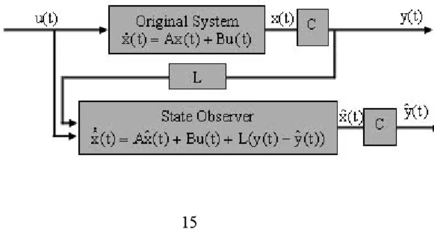
Many control systems are based on the supposition that the full state vector is available for direct measurement, but in practice, not always all the variables are avai-lable, and those unavailable must be estimated. In such a way, an observer can be built to estimate them. The schematic is as follows:

(10)

16

The observer is basically a copy of the original system; having the same input and almost the same differential equation. An extra term compares the actual measured output y(t) to the estimated output

yˆ

t(

)

.

Control systems using state observers can reconstruct the non-measured states or to estimate the values of points of difficult access in the system. However, the necessa-ry condition for this reconstruction is that all the states should be observable (Luenber-ger, 1964; D’Azzo and Houpis, 1988).

The Fig. 3 shows a logical diagram for faults detection and location in mechanical systems using the state observers' technique.

Figure 3: Observation System.

In the system of Fig. 3, when a certain component begins to fail, the state observer is capable to detect the influence of this fault quickly, because the observer is quite sensitive to any incipient irregularity that appears in the system. The state observer is a group of ordinary differential equations of first order that represents the same response as that of the real system, when it is working property. Therefore, the idea is to use this effect sensed for the state observer to detect and to locate a possible fault in a mechanical system.

In this set of observers, the global observer has the role of verifying if the system is working properly without indications of faults, because this observer uses the same system matrix of the mechanical system analysis. Thus, the global observer can detect a possible fault or irregularity in the system in analysis if the system’s response is not coincident with the global observer's response.

If a possible fault is detected, the next step would be to locate such fault, and for this reason robust observers are used. In the robust observers' assembly are removed of system matrix the parameters subject to the faults or the parameters subject to

(11)

a reduction of its values are removed from the system matrix. This way, the robust observer's response that approaches to the response of the system with fault will be the responsible one for the location of this possible fault of the system.

A possibility remains of one or more parameters failing at the same time. In this case, the solution in agreement with Melo (1998) would be to design robust state obser-vers to reach all the parameters subject to failure.

Finally, the Unit of Logical Decision (ULD) collects and analyzes the difference

between the real system and the mountedstate observers, in order to detect and to

locate faults or irregularities in the system. This unit also analyzes the progression of possible faults of the system, and activates, when it becomes necessary, an alarm sys-tem, ready to be triggered when a determined variation in a certain parameter occurs. Methodology

The Fig. 4 shows a block diagram of the developed methodology for faults detection and location in mechanical systems using state observer’s technique. The stages of this block diagram start from finding a mathematical model of the system up to the analy-sis of the response of the system and of the observers in the ULD. The commands used in this methodology belong to the package Matlab. In a general form, the developed methodology is:

• The measurements matrix [C_me] is defined so that the system is observable using

this matrix;

• All the eigenvalues of the system in analysis should have their real parts nega-tive to guarantee stability and fast convergence.

• If the system isn’t observable, new measures should be carried out until the system becomes observable;

• The matrix of the state observer [L] is obtained using MatLab’s LQR command which is an implementation of the Ackerman’s formula to calculate optimal gains [L] and to verify the stability of the system.

(12)

18

Figure 4: Block diagram of the developed methodology.

Real system Mathematical Model Determination of [M], [C], [K], [A] Eigenvalues Selection of the system Response of the system Calculation of the observer [L] Observable? Determination of the [C_me] Eigenvalues Selection of the system Calculation of the observers Response of the Observer ULD Faults detection and location

4 Numerical simulation

A numerical example is given in this section starting from the developed methodol-ogy.

Consider the cantilever beam, shaped for the technique of the finite elements us-ing beam elements, as it is shown in Figure 5, in which a is the depth of crack located in element 2.

(13)

Figure 5: Cantilever beam: (a) for numerical application (b)representation for finite element

(a)

(b)

4.1 Initial Condition

For this example we consider L=2x10-1_{m, h=5x10}-3_{m, b=8x10}-3_{m, E=2,07x10}11_N/

m2_and_ρ=7850kg/m3_{. The simulation was carried through for an initial condition}

x₁₀(0)=0.05m. The interval of time used for this simulation 0.4 second, and was 256

sampled points were taken.

(14)

20

In the Fig. 6 Graphics 1 to 10 present, the values of displacement {x₁₀(t)} of the

sys-tem (simulated) and the values reconstructed {

x

10

(

t

)

∧

} for the state observers against time in seconds.

Firstly, as can be observed in the Graphic 1, both curves are coincident, i.e., the global observer does not detect any irregularity in the system.

In order to simulate a possible fault, a crack with a=0.25h in the element 2 of the simulated system. Thus, it is observed in Graphic 2 that the curves are not coincident any longer, i.e., the global observer detects a possible fault in the simulated system. Once detected the next step is to locate this fault. For this, a set of robust observers to the possible parameters of system subject to failure has been mounted, as can be seen in Graphics 3 to 10

(15)

It can be verified that only in Graphic 7 the curves are coincident, i.e., the robust observer mounted with a=0.25h was able to locate the fault in the simulated system again.

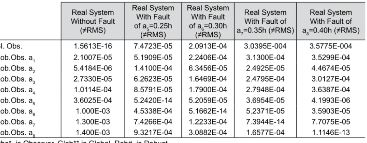
One sequence of per cent of cracks was analyzed. The values obtained are shown in the Tables 1 and 2 with present the differences of the RMS values between the real system and the global and robust state observers.

Table 1: Difference in RMS values of x₁₀(t) – Faults is a=0.05h to a=0.20h. Real System Without Fault (≠RMS) Real System With Fault of a1=0.05h (≠RMS) Real System With Fault of a2=0.10h (≠RMS) Real System With Fault of a3=0.15h (≠RMS) Real System With Fault of a4=0.20h (≠RMS)

Gl. Obs. 1.5613E-16 7.9869E-05 1.3476E-05 1.3763E-05 1.5046E-04 Rob.Obs. a1 2.1007E-05 9.0315E-14 5.0054E-05 1.6433E-05 1.5382E-04

Rob.Obs. a2 5.4184E-06 4.8098E-05 3.0070E-14 1.5468E-05 1.2639E-04

Rob.Obs. a3 2.7330E-05 1.4006E-04 7.6797E-05 1.8710E-13 7.2313E-05

Rob.Obs. a4 1.0114E-04 2.8528E-04 2.0352E-04 3.1330E-05 2.2513E-13

Rob.Obs. a5 3.6025E-04 6.4535E-04 5.7639E-04 2.3159E-04 3.2220E-04

Rob.Obs. a6 1.000E-03 1.400E-03 1.300E-03 7.8334E-04 1.000E-03

Rob.Obs. a7 1.300E-03 1.600E-03 1.600E-03 1.000E-03 1.200E-03

Rob.Obs. a8 1.400E-03 1.600E-03 1.700E-03 1.100E-03 1.300E-03

Obs*. is Observer, Glob** is Global, Rob#. is Robust

Table 2: Difference in RMS values of x₁₀(t) – Faults is a=0.25h to a=0.40h. Real System Without Fault (≠RMS) Real System With Fault of a5=0.25h (≠RMS) Real System With Fault of a6=0.30h (≠RMS) Real System With Fault of a7=0.35h (≠RMS) Real System With Fault of a8=0.40h (≠RMS)

Gl. Obs. 1.5613E-16 7.4723E-05 2.0913E-04 3.0395E-004 3.5775E-004 Rob.Obs. a1 2.1007E-05 5.1909E-05 2.2406E-04 3.1300E-04 3.5299E-04

Rob.Obs. a2 5.4184E-06 1.4100E-04 6.3456E-05 2.4925E-05 4.4674E-05

Rob.Obs. a3 2.7330E-05 6.2623E-05 1.6469E-04 2.4795E-04 3.0127E-04

Rob.Obs. a4 1.0114E-04 8.5791E-05 1.7900E-04 2.7948E-04 3.6387E-04

Rob.Obs. a5 3.6025E-04 5.2420E-14 5.2059E-05 3.6954E-05 4.1993E-06

Rob.Obs. a6 1.000E-03 4.5338E-04 5.1662E-14 5.2371E-05 3.5903E-05

Rob.Obs. a7 1.300E-03 7.4266E-04 1.2233E-04 7.3944E-14 7.7075E-05

Rob.Obs. a8 1.400E-03 9.3217E-04 3.0882E-04 1.6577E-04 1.1146E-13

Obs*. is Observer, Glob** is Global, Rob#. is Robust

In the Table 1 and 2, notice how the fault can be detected and located by comparing the global system without fault with the global observer (second line with the second