1
Abstract—This paper proposes a two-stage high order intra block prediction method for light field image coding. This method exploits the spatial redundancy in lenslet light field images by predicting each image block, through a geometric transformation applied to a region of the causal encoded area. Light field images comprise an array of micro-images that are related by complex geometric transformations that cannot be efficiently compensated by state-of-the-art image coding techniques, which are usually based on low order translational prediction models. The two-stage nature of the proposed method allows to choose the order of the prediction model most suitable for each block, ranging from pure translations to projective or bilinear transformations, optimized according to an appropriate rate-distortion criterion. The proposed higher order intra block prediction approach was integrated into an HEVC codec and evaluated for both unfocused and focused light field camera models, using different resolutions and microlens arrays. Experimental results show consistent bitrate savings, which can go up to 12.62%, when compared to a lower order intra block prediction solution and 49.82% when compared to HEVC still picture coding.
Index Terms—Light Field Image Coding, HEVC, High Order Intra Block Prediction, Geometric Transformations
I. INTRODUCTION
ight Field (LF) imaging technology available in lenslet LF cameras allows to jointly capture radiance data and angular information from the light rays hitting the camera’s sensor, by means of multiplexing the LF data in a 2D conventional sensor. This is achieved through an array of microlenses, placed between the main lens and the camera sensor. Each microlens creates a micro-image (MI) on the sensor, which is the microlens scene perspective being captured through the main lens. Therefore, a lenslet light field image tends to be like the output of an array of very small cameras.
The additional knowledge of the scene angular information allows to perform various a posteriori image processing tasks, not straightforwardly possible with traditional cameras. Refocusing and change of perspective after the picture has been taken are the most common examples [1]. These functionalities, derived from the ability to capture the “whole observable” (LF) scene [1], may be advantageous for several applications, like 3D Television [2], since by rendering several views from
The authors acknowledge the support of Fundação para a Ciência e Tecnologia, under the projects UID/EEA/50008/2013.
R. J. S. Monteiro and P. J. L. Nunes are with the Instituto de Telecomunicações, Lisbon 1049-001, Portugal, and Instituto Universitário de Lisboa (ISCTE-IUL), Lisbon 1649-026, Portugal (e-mails: ricardo.monteiro; [email protected]).
different perspectives, 2D, 3D and multiview signals can be created; image recognition and medical imaging [3].
Depending on the position of the camera sensor and the microlens array relatively to the main lens, different samplings of the light field can be performed, which define essentially the lenslet LF camera model [4]. Two main types of lenslet LF camera models exist, the unfocused [5] and the focused model [4]. In the classic unfocused camera model case, the sensor is one focal distance away from the microlens array. Thus, the microlens array is focused at infinity, i.e., the light rays that reach the microlens array are parallel [5]. Consequently, the microlens array is completely defocused from the main lens image plane. Therefore, each microlens only captures angular information, meaning that each pixel, within the MI, corresponds to a different angle, or viewpoint [5]. In the focused lenslet LF camera model, the sensor is away from the microlens array focal distance and the microlens array is focused on the main lens image plane, allowing for each microlens to generate a focused MI. This feature allows a higher spatial resolution for rendering, since more than one pixel can be extracted from each MI in the rendering process [4]. These models have been the base for the deployment of this technology, allowing an increasing number of applications and users.
The growing interest in LF technology led the JPEG Committee to launch a new activity, known as JPEG Pleno, to address coding and representation of content generated by emerging imaging technologies such as LF, point-cloud and holographic technologies [6].
The large amount of data required to adequately represent a LF scene, when compared to the case of typical 2D pictures, calls for efficient techniques for both transmission and storage of this type of content. In this context, several authors proposed specific LF coding techniques, which can be applied directly to the lenslet LF images, in order to exploit the MIs redundancy. Alternatively, other techniques are applied to a different representation of the same LF, which comprises the view point images, also known as sub-aperture images (SAIs). The SAIs are generated by extracting at least one pixel, in a fixed position, from each MI and organizing them into a matrix. Each SAI represents a rendered image, from a different perspective, extracted from the LF image.
N. M. M. Rodrigues and S. M. M. Faria are with the Instituto de Telecomunicações, Leiria 2411-901, Portugal, and Escola Superior de Tecnologia e Gestão, Instituto Politécnico de Leiria, Leiria 2411-901, Portugal (e-mails: nuno.rodrigues; [email protected]).
Light Field Image Coding using High Order
Intra Block Prediction
Ricardo J. S. Monteiro, Student member, IEEE, Paulo J. L. Nunes, Member, IEEE, Nuno M. M. Rodrigues, Member, IEEE and Sérgio M. M. Faria, Senior Member, IEEE
2 State-of-the-art LF coding schemes rely on block matching
techniques to exploit the inherent spatial redundancy in lenslet LF images. However, these low order prediction (LOP) models use only two degrees of freedom (DoF), as only translations are used to describe the inherent LF image spatial redundancy.
Due to the small baseline between MIs in lenslet LF images, the different MIs can be approximately related by changes in perspective, which require eight DoF to be described. To the best of authors’ knowledge, this characteristic has not been exploited by previous LF coding approaches described in the literature. This additional matching accuracy is important to develop a coding method able to cope with important features of the LF content, such as:
1) The LF camera model, i.e., both focused and unfocused models should be handled;
2) The type of microlens array structure, e.g., rectangular or hexagonal microlens layouts, creating rectangular, hexagonal or circular MIs;
3) The MI size, i.e., a parameter that depends on the camera, and has a strong influence on the number of possible rendered points of view and their spatial resolution. High order prediction (HOP) models, e.g., using geometric transformations with more DoF, have been studied during the last two decades in traditional 2D and 3D image coding scenarios. Several geometric models, like translation, rotation, scale, shear and perspective changes have been used to improve the coding efficiency, by exploiting spatial [7], temporal [8]– [13] and inter-view [14]–[17] redundancy. In most proposals, these models have been applied image-wise (instead of block-wise), due to two main reasons: (i) high computational complexity in block-wise model parameter estimation, and (ii) significant additional bit rate required for parameter transmission. Despite these drawbacks, this paper demonstrates that block-wise HOP models can increase block matching accuracy and, thus, coding efficiency for lenslet LF images.
The method proposed in this paper for encoding lenslet LF images relies on a two-stage block-wise HOP model, where each image block is intra predicted from a reference in the causal area of the image, i.e., containing pixels that were already encoded. Since this approach is applied block-wise, it is possible to optimize the HOP model (number of DoF) for each block to be encoded. Taking advantage of the extra DoF available in HOP models, it is possible to outperform state-of-the-art coding techniques based on LOP models.
The remainder of this paper is organized as follows: Section II presents a review of several relevant state-of-the-art solutions, regarding LF image coding; Section III describes the geometric transformations used in the proposed prediction method; Section IV presents the proposed HOP model; Section V presents the test conditions and experimental results; and, finally, Section VI concludes the paper.
II. RELATED WORK ON LIGHT FIELD IMAGE CODING Several schemes to encode lenslet LF images are described in the literature, aiming to exploit the intra-LF image redundancy. These schemes rely on different LF image representations and coding techniques, which may be categorized according to the fundamental adopted approach as:
transform-based coding, pseudo-video sequence coding, disparity-based coding and non-local spatial prediction coding. A. Transform-based coding
Some LF coding schemes rely, essentially, on the use of a transform, mainly the discrete cosine transform (DCT) [18], [19] or the discrete wavelet transform (DWT) [20]. In [18], a 3D-DCT is applied to a stack of MIs, to exploit the existing spatial redundancy within a MI, as well as the redundancy between adjacent MIs. In [20], a LF image is decomposed into SAIs, and a 3D-DWT is applied to a stack of these SAIs. The lower frequency bands are transformed using a two-dimensional discrete wavelet transform (2D-DWT), while the remaining higher frequency coefficients are simply quantized and arithmetic encoded. These coding schemes are reportedly more efficient than JPEG, but not as efficient as HEVC still picture coding.
B. Pseudo-video sequence coding
This type of LF coding schemes represent the LF image as a set of MIs or SAIs, and re-organize them into a low resolution pseudo-video sequence (PVS), which is then compressed using a standard video encoder. Various scanning strategies to order the PVS are considered to better exploit the redundancy between MIs or SAIs. Dai et al. [21] propose to scan the SAIs using either a raster or a spiral scan and then encode the generated video sequence with H.264/AVC. Vieira et al. [22] used similar scanning strategy combined with several prediction structures supported by HEVC. In both cases it is possible to conclude that the spiral scan is more efficient than the raster scan. More recently, in the ICME light field compression challenge [23], Liu et al. [24] used a PVS scheme to organize the SAIs into layers, depending on the proximity to the central view, starting with the central SAI and moving on to the outer views. The more distant the SAI is from the center, the higher the value of the used quantization parameter (QP) should be. This scheme was implemented using both HEVC test model (HM) and JEM [25] software. Because the rate allocation is not uniform along the LF image, this method is prone to reconstruct views with different objective qualities.
C. Disparity-based coding
In this type of LF coding schemes the LF image is considered as a set of views captured by different cameras (either in the form of MIs or SAIs), which may be encoded exploiting inter-view disparity. In [26], the authors propose a coding method that uses some SAIs to calculate a set of disparity maps prior to coding, which are then used to predict the remaining SAIs. The authors concluded that this approach is suitable to encode synthetic images, where disparity compensation alone can be enough to predict a SAI. A compression scheme that incorporates disparity compensation into 4D wavelet coding using disparity compensated lifting is proposed in [27]. The disparity information derived from an approximated model of the scene is applied to modify the update and prediction filters of the lifting procedure. In [28], the authors propose a scalable (two-layer) LF coding approach for the focused LF camera model, using a LF representation that consists of a sparse set of
3
MIs and associated disparity maps. Based on the sparse set of MIs and the associated disparity maps (first layer), a reference prediction LF image is obtained through a reconstruction method that relies on disparity-based interpolation and inpainting. This reconstructed LF image is then used to encode the original LF image (second layer), by encoding the prediction residue. This approach was later extended [29] with a third layer of scalability and the use of lossy encoded disparity maps, in contrast with the lossless transmission of the disparity maps, used in the first approach. Both versions of the work are able to outperform HEVC still picture coding.
D. Non-local spatial prediction coding
Several methods to exploit the non-local spatial redundancy were proposed as additional coding tools for existing video coding standards, like HEVC. In [30], a self-similarity compensated prediction is proposed to take advantage of the flexible partition patterns used by this video codec. In [31] this method was extended with a bi-directional mode to increase its coding efficiency. Additionally, in [32], an alternative non-local spatial prediction method has been investigated, relying on a prediction mode based on locally linear embedding integrated in HEVC. Differently from the other schemes, that exploit non-local spatial redundancy, this method distributes the computational complexity between the encoder and the decoder, i.e., the locally linear embedding procedure must be replicated in the decoder. In [33] the authors developed a multi-hypothesis coding method specifically for focused LF image and video. This method uses up to two hypotheses for prediction in both spatial and time domains, which outperforms single-hypothesis based prediction. For the unfocused camera model, the authors concluded that the rate-distortion efficiency is still much higher, compared to JPEG or HEVC, however the gains relatively to HEVC are smaller in this case when compared to the focused model [34].
The main advantage of this category is that, in most approaches, the lenslet LF images are encoded without the need of any pre-processing steps or any prior knowledge about the capturing device, e.g., the LF camera model, the microlens array structure and the MI size.
III. GEOMETRIC TRANSFORMATIONS FOR HIGH ORDER PREDICTION
In most state-of-the-art encoders, prediction between blocks of pixels is performed using very simple transformations, like translations. However, a lenslet LF image is comprised of MIs that are related by more complex transformations, resulting from the fact that each MI represents the scene being captured from slightly different perspectives. In such cases, it is
advantageous to use geometric transformations that better exploit the features of the LF image and its MIs.
A geometric transformation (GT) is able to map perspective changes from one view (generically associated to a quadrilateral) into another view, requiring up to eight DoF.
Considering two different blocks, 𝐴 and 𝐴′, each one with its own coordinate system, (𝑢, 𝑣) and (𝑥, 𝑦), respectively, it is possible to define a generic relationship:
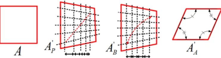
(𝑥, 𝑦) = +𝑋(𝑢, 𝑣), 𝑌(𝑢, 𝑣)., (1) where 𝑋 and 𝑌 are mapping functions for each coordinate. These functions create a point to point correspondence between images. Depending on the number of DoF used by the mapping functions in (1), different number of independent point to point correspondences are possible. To describe these mapping functions, some GTs may be used, namely, Projective, Bilinear or a simpler Affine GT, as illustrated in Fig. 1.
A. Projective geometric transformation
In order to simplify the mathematics used in this kind of GT, homogeneous coordinates are commonly used [35]. Thus, the Projective GT can be defined by a 3×3 matrix 𝑯 verifying (2):
[𝑥, 𝑦, 1] = [𝑢ℎ, 𝑣ℎ, ℎ]𝑯 . (2) The Projective matrix 𝑯 can be decomposed into three different submatrices, 𝑳𝒑, 𝑻𝒑 and 𝑷𝒑:
𝑯 = 8𝑳𝑻𝒑 𝑷𝒑 𝒑 1 9 𝑳𝒑= 8𝑙𝑙;; 𝑙;< <; 𝑙<<9, 𝑻𝒑 = [𝑡> 𝑡?], 𝑷𝒑𝑻= [𝑝> 𝑝?] (3)
Each submatrix is responsible for a different elementary type of GT: 𝑻𝒑 is responsible for the description of translations, 𝑳𝒑 is able to define linear transformations such as rotation, scaling, and shearing, and 𝑷𝒑 describes perspective transformations.
To fully exploit the capabilities of the projective matrix 𝑯, a four-point correspondence is necessary between blocks 𝐴 and 𝐴′. In this case, the full transformation matrix corresponds to the following system of equations:
⎩ ⎪ ⎨ ⎪ ⎧𝑥 = 𝑋(𝑢, 𝑣) =𝑙;;𝑢 + 𝑙<;𝑣 + 𝑡> 𝑝>𝑢 + 𝑝?𝑣 + 1 𝑦 = 𝑌(𝑢, 𝑣) =𝑙;<𝑢 + 𝑙<<𝑣 + 𝑡? 𝑝>𝑢 + 𝑝?𝑣 + 1 (4)
The system of equations (4) defines the necessary calculations for mapping the coordinates of every pixel of block A into the transformed block 𝐴′.
The number of available DoF is directly related with the number of known points of correspondence which exist between both images. For less than four points of correspondence, simpler transformations can be represented by the perspective model. For example, if one point is known, the only component that can be possibly described is a translation, i.e., 𝑻𝒑 = F𝑡>, 𝑡?G, 𝑷𝒑= [0,0]I and 𝑳𝒑= 𝑰. This case is defined by (5):
Fig. 1 - Examples of possible GTs applied to block 𝐴: Projective (𝐴KL),
4
[𝑥, 𝑦, 1] = [𝑢ℎ, 𝑣ℎ, ℎ] 8𝑻𝑰 𝟎
𝒑 19, (5)
which can be translated into the system of equations (6): O𝑥 = 𝑋(𝑢) = 𝑢 + 𝑡>
𝑦 = 𝑌(𝑣) = 𝑣 + 𝑡?. (6)
B. Bilinear geometric transformation
The Bilinear GT is an alternative to the Projective GT, defined by a 4×2 matrix 𝑩 verifying (7):
[𝑥, 𝑦] = [𝑢𝑣, 𝑢, 𝑣, 1]𝑩, (7) where: 𝑩 = Q 𝑷𝒃 𝑳𝒃 𝑻𝒃 S = T 𝑝> 𝑝? 𝑙;; 𝑙;< 𝑙<; 𝑙<< 𝑡> 𝑡? U, (8)
The Bilinear GT matrix 𝑩 can represent similar GTs as the Projective GT, with the same number of DoF. However, it performs a non-planar transformation, which makes it more flexible. Thus, only horizontal and vertical lines, as well as equispaced points along these directions, are preserved [36]. Diagonal lines, on the other hand, are not mapped as lines but as quadratic curves. This feature is illustrated in Fig. 1, where, in the case of the Bilinear GT, points along vertical parallel lines are kept equispaced, while the points along diagonal lines are mapped onto a quadratic curve (block 𝐴M). When the Projective GT (block 𝐴V) is used, points along the parallel vertical lines do not stay equispaced but points along diagonal lines are also mapped along a line. Another property of this GT, when compared to the Projective GT, is the need for simpler calculations per pixel, given by (9):
O𝑥 = 𝑋(𝑢, 𝑣) = 𝑢𝑣𝑝𝑦 = 𝑌(𝑢, 𝑣) = 𝑢𝑣𝑝>+ 𝑢𝑙;;+ 𝑣𝑙<;+ 𝑡>
?+ 𝑢𝑙;<+ 𝑣𝑙<<+ 𝑡?. (9)
C. Affine geometric transformation
When using either the Projective or the Bilinear GT, eight DoF are available. However, a simpler case exists, which is known as the Affine GT, that is able to describe GTs up to six
DoF. The Affine GT can be described as a particular case of Projective or Bilinear GTs, by using matrices 𝑯 and 𝑩 with 𝑷𝒑𝑻= [0 0] and 𝑷𝒃= [0 0], respectively. This GT only requires three points of correspondence between images, defined by (10):
O𝑥 = 𝑋(𝑢, 𝑣) = 𝑙𝑦 = 𝑌(𝑢, 𝑣) = 𝑙;;𝑢 + 𝑙<;𝑣 + 𝑡>
;<𝑢 + 𝑙<<𝑣 + 𝑡?. (10) IV. PROPOSED HIGH ORDER PREDICTION MODE This section proposes a LF image coding method, based on a high order prediction model, which is implemented as a block-wise prediction mode in HEVC. This HOP mode is added to the set of HEVC Intra prediction modes, i.e., Planar mode, DC mode and the 33 intra Directional modes.
The proposed HOP mode predicts each block by applying a GT between two quadrilaterals, the current block and a block in the reference region, the causal area of pixels already encoded. The algorithm for the proposed prediction mode can be described through the following steps:
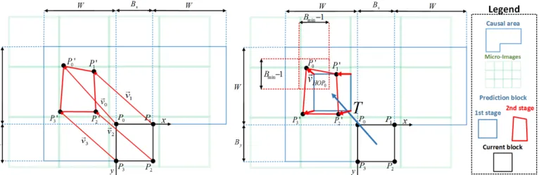
1) Selection of the next set of correspondence points to be evaluated: Selection of a quadrilateral in the causal area of pixels (from a set of pre-defined cases), with corners {𝑃ZL}, that is mapped into the block which is being predicted, with corners {𝑃Z} (see left side of Fig. 2); 2) Calculation of the GT parameters: Calculation of the
transformation parameters that map the quadrilateral defined by {𝑃ZL} into the one defined by {𝑃Z};
3) Inverse GT mapping: Mapping of the causal quadrilateral defined by {𝑃ZL} to the one defined by {𝑃Z}, using an inverse mapping procedure with the parameters calculated in the previous step, in order to compute the block prediction error; error and the estimated number of bits to transmit the GT parameters;
4) Estimation of the GT RD cost: Estimation of the rate-distortion (RD) cost, J, associated to the GT that is being evaluated, considering the computed block prediction; 5) Repeat the above steps to find the GT with minimum RD
cost: Evaluate iteratively all the pre-defined combinations of correspondence points and choose the one that has the minimum RD cost 𝐽.
IEEE Journal on Selected Topics in Signal Processing (JSTSP) - Special Issue on Light Field Image Processing 5
6) Encode the HOP mode information: The corner displacement between the quadrilateral in the causal area {𝑃ZL} and the block which is being predicted {𝑃Z} is signaled to the decoder.
The following sub-sections explain each step of the proposed HOP mode in more detail.
A. Selection of the correspondence points
The major challenges faced by the proposed algorithm are the computational complexity required to estimate the optimal set of GT parameters and the necessary bit-rate for transmitting this data. To tackle both problems, a rate-distortion-complexity tradeoff is defined. From Fig. 2 (left side) it can be inferred that, if all possible four-point correspondences between the prediction block and the current block to be encoded were evaluated, the number of tested transformations per block would be larger than (2𝑊`)a, i.e., for a search window (𝑊 = 128) more than 1.15 × 10<e correspondence possibilities per block exist. To reduce the number of tests to a practicable number, a two-stage minimization problem is proposed, aiming to determine a good approximation to the optimal HOP model, as illustrated in Fig. 2 (right side):
1) LOP Model Estimation
In the first stage, a pure translational LOP model (two DoF) is used. The result of this stage is, the bidimensional vector, 𝑻, with the lowest RD cost, pointing into the search window of the causal area (see the blue vector on the right side of Fig. 2). The search to determine 𝑻 is performed using a full search algorithm, as described in [30]. The LOP estimation stage of the proposed HOP mode is based on the Self Similarity (SS) prediction method. The prediction cost is minimized by testing all the possible positions inside the search window for a single vector that relates the current block to the prediction block. The 𝑻 vectors, generated by the first stage, can be either encoded explicitly, similarly to motion vectors in HEVC or using the SS-Skip mode, which creates a list of candidates that includes the 𝑻 vectors used to encode neighboring blocks. If one candidate from this list is selected to encode the current block, it is only necessary to encode the its index, as in the HEVC merge mode. Additionally, some predetermined vectors are added to the candidate list, referred to as MI-based candidates [30]. These candidates correspond to vectors that are very likely to be
selected by the SS prediction mode, such as, vectors pointing to the same spatial position of the current MI within the left, above and above-left MIs.
2) HOP Model Estimation
In the second stage, a HOP model (up to eight DoF) is used, employing as a starting point the result of the first stage (see, respectively, the red and blue quadrilaterals on the right side of Fig. 2). For this, a set of four vectors, f𝑣ghKij, is computed, each of them defining the position of one corner of the reference quadrilateral, thus defining the 2D GT.
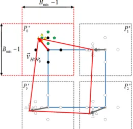
To further reduce the computational complexity of the second stage of this minimization problem, a 2D logarithmic fast search method has been adopted, which is applied to each corner of the prediction block (blue rectangle). In this case, the maximum number of search steps has been set to 𝑙𝑜𝑔`+𝑚𝑖𝑛(𝐵>, 𝐵?). − 1, depending on the size of the prediction block, i.e., 𝐵> (width) and 𝐵? (height). In each step, the searching points are defined according to a five-point small diamond-shaped basis pattern with an initial search step size equal to 𝑚𝑖𝑛(𝐵>, 𝐵?)/4 [37], [38]. This 2D logarithmic fast search method using the five-point small diamond-shaped basis pattern is graphically represented in Fig. 3 across three search steps, represented, respectively, by black circles, green pentagons and yellow triangles. After each search step, the point that minimizes the RD cost function is set as the center of the next step and the search step size is halved until a unitary step value is reached. In the example of Fig. 3, in the first corner (𝑃;), the five points associated with the first step, represented by the black circles, are tested. The point that minimizes the RD cost function for the first search step is the black circle on the top. For the second and third search steps, the points on left, respectively, green pentagon and yellow triangle, are the points that yield the lowest RD cost. The final point is selected to define the red arrow that describes the corner displacement of the first corner of the block.
Considering that the search procedure must be applied to all the corners of the prediction block over several search steps, there are two ways of implementing this second stage search: by jointly optimizing each step of the search procedure for the four corners or by independently optimizing each step of the search procedure. By considering five points for each of the S search steps of the 2D logarithm search, the required number of search points for each option is given by (5 × 𝑆)Z or 5Z× 𝑆, respectively where 𝑛 is the number of corners. In order to reduce the computational complexity, the second option was used, where each step is optimized individually.
The stop condition for this search method is met when the corner step size reaches the unit. Therefore, the example shown in Fig. 3 represents the unitary steps as the yellow triangles. Since the underlying codec uses variable block sizes, 𝑆 will depend on the block size. The search window for each corner is limited to 𝑚𝑖𝑛+𝐵>, 𝐵?. − 1, as illustrated in Fig. 3 (see the dashed red block).
The quadrilateral used by the HOP model estimation may be scaled to increase pixel precision. Fig. 2 and Fig. 3 illustrate the second stage applied to a blue rectangle with the same size of the block being predicted (in black) to not overload the figures. However, in our implementation, a rectangle, twice the size of the original block, is used to determine the HOP model. This
Fig. 3 – Fast search method adopted for each corner of the prediction block (blue rectangle) used to estimate the HOP model (red quadrilateral).
IEEE Journal on Selected Topics in Signal Processing (JSTSP) - Special Issue on Light Field Image Processing 6
modification means that an integer pixel displacement in one of the corners of the large quadrilateral corresponds to a sub-pixel displacement in the area of the original rectangle. For a block twice the size of the original block, one extra search step is performed by the 2D logarithmic search algorithm that is used at the HOP stage. This occurs because the stopping condition for the search algorithm is the unitary step size. The pixel precision can be further extended by using a rectangle with sides four or eight times the size of the original blue rectangle, which increase, the number of search steps by one or two, respectively. After extensive testing, the best solution in a RD sense was adopted, that is increasing the blue rectangle to twice the original size, despite requiring one extra step.
As the second stage of the HOP search can be biased by the first stage result, the global result of the search method also tests the 𝑻 vectors used in the previously encoded neighboring blocks (vector predictors), instead of considering only the best 𝑻 vector from the first stage. Additionally, other 𝑻 vectors can be tested in conjunction with the HOP model estimation, e.g. top ten candidates from the first stage. However, it was experimentally verified by the authors that the vectors that are more RD cost efficient are the 𝑻 vector predictors.
The proposed approach can be implemented using either the Projective GT defined in (3): 𝑯 = u𝟎 𝟎𝑻 0v + w𝑳𝒑 L 𝑷 𝒑 L 𝑻𝒑L 1x = w 𝑳𝒑L 𝑷𝒑L 𝑻 + 𝑻𝒑L 1x (11) or the Bilinear GT defined in (8):
𝑩 = Q𝟎𝟎 𝑻S + y 𝑷𝒃L 𝑳𝒃L 𝑻𝒃L z = y 𝑷𝒃L 𝑳𝒃L 𝑻 + 𝑻𝒃L z . (12)
Where 𝑻 is the vector estimated during the LOP stage and 𝑻′, 𝑳′ and 𝑷′ are the GT parameters that describe the HOP stage. B. Calculation of the GT parameters
After obtaining vector 𝑻 (see the right side of Fig. 2), it is possible to determine submatrices 𝑻L, 𝑷L and 𝑳L in equations (11) and (12), by using their width and height, 𝐵> and 𝐵?, respectively, and the small vectors associated with the corner position change of the blue rectangle:
⎩ ⎪ ⎨ ⎪ ⎧𝑣⃗ghK|= (𝑢;, 𝑣;) 𝑣⃗ghK}= (𝑢<− (𝐵>− 1), 𝑣<) 𝑣⃗ghK~= (𝑢`− (𝐵>− 1), 𝑣`− (𝐵?− 1)) 𝑣⃗ghK•= (𝑢€, 𝑣€− (𝐵?− 1)) (13)
Note that in the proposed two-stage approach, vectors 𝑣⃗Z, represented in the left of Fig. 2, correspond to the sum of vector 𝑻 from the first stage, with the four smaller vectors from the second stage, i.e.,𝑣⃗Z= 𝑇 + 𝑣⃗ghKi , represented in the right of Fig. 2. If the Projective GT is used some auxiliary variables are defined: ‚Δ𝑢Δ𝑢<`= 𝑢= 𝑢<€− 𝑢− 𝑢`` Δ𝑢€= 𝑢;− 𝑢<+ 𝑢`− 𝑢€ ‚Δ𝑣Δ𝑣<`= 𝑣= 𝑣<€− 𝑣− 𝑣`` Δ𝑣€= 𝑣;− 𝑣<+ 𝑣`− 𝑣€ . (14)
The Affine GT can be defined by any three of the four vectors (𝑣⃗ghK). In this paper, the first three vectors, 𝑣⃗ghK|, 𝑣⃗ghK}and 𝑣⃗ghK~ are generated using the second stage of the proposed
approach, where the remaining vector, 𝑣⃗ghK•, is calculated
assuming 𝛥𝑢€= 𝛥𝑣€= 0, thus resulting in 𝑣⃗ghK•= (𝑢;− 𝑢<+ 𝑢`, 𝑣;− 𝑣<+ 𝑣`− (𝐵?− 1)).Using (14), the individual parameters in the submatrices can then be calculated by (15) for the Projective GT: 𝑷𝒑L = ⎣ ⎢ ⎢ ⎢ ⎢ ⎡ < Mˆ‰< Š‹Œ‹•• ‹Œ~ • ‹•~Š Š‹Œ‹•} ‹Œ~ } ‹•~Š < MŽ‰< Š‹Œ‹•} ‹Œ• } ‹••Š Š‹Œ‹•} ‹Œ~ } ‹•~Š⎦ ⎥ ⎥ ⎥ ⎥ ⎤ and 𝑳𝒑L = ⎣ ⎢ ⎢ ⎡𝑢𝐵<− 𝑢; >− 1 + 𝑝>𝑢< 𝑢€− 𝑢; 𝐵?− 1 + 𝑝?𝑢€ 𝑣<− 𝑣; 𝐵>− 1 + 𝑝>𝑣< 𝑣€− 𝑣; 𝐵?− 1 + 𝑝?𝑣€⎦ ⎥ ⎥ ⎤ . (15)
Similarly, for the Bilinear GT, the corresponding submatrices are calculated by (16):
𝑷𝒃L𝑻= y Œ|‰Œ}’Œ~‰Œ• (Mˆ‰<)+MŽ‰<. •|‰•}’•~‰•• (Mˆ‰<)+MŽ‰<. z and 𝑳𝒃L = y Œ•‰Œ| MŽ‰< ••‰•| MŽ‰< Œ}‰Œ| Mˆ‰< •}‰•| Mˆ‰< z. (16)
For both cases we have:
𝑻𝒑L = 𝑻𝒃L = [𝑢; 𝑣;]. (17)
C. Inverse GT mapping
As previously mentioned, a GT between two blocks corresponds to a mapping of every pixel within one block into the other block, e.g., the mapping functions (4) and (9) correspond to the Projective and Bilinear GT, respectively. When the mapping is performed from the rectangular block to
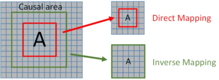
Fig. 4 - Example of Direct Mapping and Inverse Mapping when a scale GT is applied.
IEEE Journal on Selected Topics in Signal Processing (JSTSP) - Special Issue on Light Field Image Processing 7
be encoded to an arbitrary reference quadrilateral it is called a direct mapping, otherwise it is called an inverse mapping. An example of how both mapping procedures for a simple scaling GT can be found in Fig. 4. As can be observed in Fig. 4, when direct mapping is used the final quadrilateral shape (red block) does not match the desired reference block pixel grid, requiring to perform pixel interpolation prior to calculate the distortion between the transformed block and the reference block. For the sake of simplicity, an inverse mapping has been adopted, as it generates a rectangular prediction block with the same dimensions of the block to be encoded.
Thus, regardless of the size of the quadrilateral used for estimation, (4) and (9) take as input the coordinates of the block to be encoded, i.e., 𝑢 ∈ [0, 𝐵>− 1] and 𝑣 ∈ F0, 𝐵?− 1G, and generate as output the coordinates (𝑥, 𝑦) in the causal area, where the reference pixel value is going to be extracted from. Since 𝑥 and 𝑦 are typically fractional values, a bilinear interpolation filter is used to compute the actual pixel value. D. Estimation of the GT RD cost
The optimal HOP model for each block is determined through RD optimization, minimizing the associated Lagrangian cost, 𝐽 = 𝐷 + 𝜆𝑅, over the entire set of pre-defined GT. 𝐷 refers to the distortion between the prediction block and the current block, 𝑅 is the estimated number of bits used to encode the block using the GT under evaluation, and 𝜆 is the Lagrange multiplier, computed as in HM version 15.0 for Intra-coded frames. The parameter 𝜆 is the same for all prediction modes, including the intra modes, so no biases in terms of prediction mode selection are introduced. In this paper, 𝐷, is computed as the sum of absolute differences (SAD) in the pixel domain, in the first stage, and SAD in the Hadamard domain, in the second stage, as suggested in [39].
By using a two-stage method it is possible to evaluate if it is more advantageous to use LOP or HOP for each block, by comparing the associated costs, given by:
𝐽—hK= 𝐷—hK+ 𝜆𝑅—hK, and 𝐽ghK= 𝐷ghK+ 𝜆𝑅ghK ,
(18)
where 𝑅—hK and 𝑅ghK are the estimated number of bits for the corresponding coding mode.
The usage of LOP or HOP is conveyed to the decoder through a binary flag, 𝐹ghK. When LOP is considered more efficient in a RD sense, 𝐹ghK= 0, and only 𝑻 is transmitted in the bitstream. On the contrary, if HOP is used, all the elements that describe 𝑻 are transmitted, followed by 𝐹ghK= 1 and the four additional 𝑣⃗ghKi vectors.
The number of bits required to signal the HOP mode, 𝑅ghK, is the sum of 𝑅—hK and the estimated bits for encoding the four vectors, 𝑣⃗ghKi, that define the used HOP model. The rate of
these small amplitude vectors is estimated using the same procedure as vector 𝑻.
E. Encode the HOP mode information
After finding the optimal HOP model, the cost of the HOP mode, 𝐽ghK, is compared against the cost of the other intra prediction modes, i.e., DC, Planar and the 33 Directional modes, and the mode with the lowest RD cost is encoded. For this, the context adaptive binary arithmetic coding (CABAC) entropy coding method used by HEVC is used to encode the HOP mode information. The CABAC entropy coder is based on three steps: (i) binarization of syntax elements, (ii) context modeling, and (iii) binary arithmetic coding. In this implementation, these three steps have been maintained using, however, new contexts. Vectors 𝑻 and 𝑣⃗ghKi, and flag, 𝐹ghK,
are transmitted to the decoder using the HM approach for motion vectors and merge flags [40].
To encode 𝑻, the same syntax elements of HEVC for motion data are used, i.e., motion vector differences, MVP index, reference picture list (RPL) and RPL index.
The way the HOP model information is conveyed to the decoder can highly influence the coding efficiency. One possible approach is to send the GT parameters, i.e., in the 𝑯 or 𝑩 matrix, which need to be represented with high precision. Alternatively, as proposed in this paper, the encoder just sends the four vectors, 𝑣⃗ghKi, which can be represented with just a
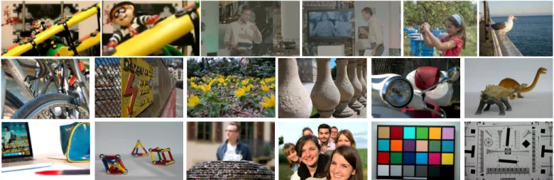
few bits. The major advantage of encoding the GT parameters matrix is that they do not need to be recalculated at the decoder side through equations (13) – (17). However, they need to be encoded with a very high precision because these values are not Fig. 5 - LF test images part of the experimental test setup. First row (from left to right): Plane and Toy (frame 0 and 150), Demichelis Spark (frame 0),
IEEE Journal on Selected Topics in Signal Processing (JSTSP) - Special Issue on Light Field Image Processing 8 TABLE I
BD-PSNR-Y AND BD-RATE RESULTS COMPARING HEVC,HEVC-SS(TWO DOF) AND HEVC-HOP, USING SIX DOF AND EIGHT DOF AND TWO DIFFERENT KINDS OF GEOMETRIC TRANSFORMATIONS Image HEVC-SS (2 DoF) vs HEVC HEVC-HOP-A (6 DoF) vs HEVC-SS (2 DoF) HEVC-HOP-P (8 DoF) vs HEVC-SS (2 DoF) HEVC-HOP-B (8 DoF) vs HEVC-SS (2 DoF) BD-
PSNR-Y BD-RATE PSNR-Y BD- BD-RATE PSNR-Y BD- BD-RATE PSNR-Y BD- BD-RATE Plane and Toy, frame 0 (PT0) 0.90 dB -14.64 % 0.23 dB -3.93 % 0.27 dB -4.66 % 0.23 dB -4.02 % Plane and Toy, frame 150 (PT150) 1.44 dB -19.02 % 0.64 dB -9.44 % 0.75 dB -11.05 % 0.71 dB -10.50 % Demichelis Spark, frame 0 (DS) 1.09 dB -31.43 % 0.23 dB -7.41 % 0.26 dB -8.39 % 0.26 dB -8.31 % Demichelis Cut, frame 0 (DC) 1.05 dB -29.25 % 0.26 dB -8.06 % 0.30 dB -9.14 % 0.29 dB -8.83 % Laura (LAURA) 2.26 dB -30.35 % 0.15 dB -2.76 % 0.27 dB -4.78 % 0.32 dB -5.62 %
Seagull (SEAGULL) 2.81 dB -42.78 % 0.22 dB -4.89 % 0.31 dB -6.82 % 0.43 dB -9.21 %
Bikes (BIKES) 0.81 dB -18.50 % 0.11 dB -2.91 % 0.13 dB -3.34 % 0.11 dB -2.97 % Danger de Mort (DANGER) 0.61 dB -14.67 % 0.10 dB -2.72 % 0.11 dB -2.94 % 0.10 dB -2.75 % Flowers (FLOWERS) 0.17 dB -4.10 % 0.03 dB -0.75 % 0.03 dB -0.77 % 0.03 dB -0.67 % Stone Pillars (STONE) 0.25 dB -6.31 % 0.02 dB -0.61 % 0.02 dB -0.57 % 0.02 dB -0.57 % Vespa (VESPA) 0.89 dB -28.73 % 0.10 dB -3.90 % 0.14 dB -5.30 % 0.12 dB -4.89 % Ankylosaurus & Diplodocus (ANKY) 1.43 dB -45.35 % 0.05 dB -1.26 % 0.06 dB -4.46 % 0.05 dB -2.91 % Desktop (DESKTOP) 0.48 dB -13.73 % 0.26 dB -8.05 % 0.25 dB -7.78 % 0.29 dB -8.93 %
Magnets (MAGNTES) 0.66 dB -22.95 % 0.06 dB -3.52 % 0.06 dB -5.19 % 0.05 dB -2.62 % Fountain & Vincent (FOUNTAIN) 1.49 dB -30.72 % 0.17 dB -4.39 % 0.20 dB -5.31 % 0.20 dB -5.28 % Friends (FRIENDS) 0.22 dB -8.10 % 0.05 dB -2.01 % 0.06 dB -2.21 % 0.06 dB -2.36 %
Color chart (COLOR) 1.49 dB -42.84 % 0.27 dB -11.19 % 0.31 dB -12.30 % 0.32 dB -12.62 %
ISO Chart (ISO) 1.42 dB -41.35 % 0.24 dB -9.28 % 0.27 dB -10.42 % 0.27 dB -10.47 %
AVG. FOC 1.59 dB -27.91 % 0.29 dB -6.08 % 0.36 dB -7.47 % 0.37 dB -7.75 %
AVG. UNF 0.83 dB -23.11 % 0.12 dB -4.22 % 0.14 dB -5.06 % 0.14 dB -4.75 % AVG. ALL 1.08 dB -24.71 % 0.18 dB -4.84 % 0.21 dB -5.86 % 0.21 dB -5.75 %
very robust to quantization [11]. Consequently, encoding the vectors, 𝑣⃗ghKi, leads to higher compression efficiency.
V. EXPERIMENTAL RESULTS
In this section the performance of the proposed lenslet LF coding solution, incorporating the HOP mode, is evaluated in comparison with state-of-the-art coding solutions based on LOP approaches. First, this section describes the test conditions, including the used lenslet LF test images, the benchmark solutions and the relevant test parameters. Afterwards, experimental results comparing the RD performance of different types of prediction models are presented and discussed. These results are complemented with some statistical information about prediction mode usage and an evaluation of the quality of the rendered views, as proposed in [23], using the coded LF images.
A. Test conditions
In order to evaluate the RD performance of the proposed LF coding solution, two types of LF images were selected for the experimental test setup. The first type of images were acquired using LF cameras with a focused (FOC) optical setup [41], [42]. The second type of images were acquired using a Lytro Illum camera that is commercially available and uses an unfocused (UNF) optical setup. This second set of images constitutes the dataset used for the 2016 ICME Grand Challenge on LF image compression extracted from the EPFL dataset [23]. The central rendered views of all the test images are shown in Fig. 5, where
the first row corresponds to the first type of images and the second and third rows correspond to the second one. This selection includes LF images with different resolutions, MI resolutions and types of microlens arrays, with different MI shape. Plane and Toy images have a resolution of 1920×1088 (MIs 28×28); Demichelis images have a resolution of 2880×1620 (MIs 38×38); Laura and Seagull have a resolution of 7240×5432 (MIs 75×75); EPFL images have a resolution of 7728×5368 pixels (MIs 15×15).
The proposed HOP mode was implemented into the HEVC test model version 15.0 (HM 15.0) as an additional intra prediction mode. This LF codec, corresponding to the proposed solution, will be referred to as HEVC-HOP, where HEVC using only the standard Intra modes is simply referred to as HEVC. Additionally, the work in [30] is used as benchmark for RD performance and it is referred to as HEVC-SS.
The common HM test conditions were adopted, using QP values of 22, 27, 32 and 37. The causal window size 𝑊 is 128 for both HEVC-HOP and HEVC-SS, for every encoded image. The number of available SS or 𝑻 vector predictors, used for coding, is 2. These 𝑻 vector predictors are used as additional vector 𝑻 candidates for the LOP model estimation stage. As mentioned in the previous section, these alternative vectors are tested in order to have a more unbiased result when estimating the HOP model. The number of candidates available for SS-Skip is 5 in both HEVC-SS and HEVC-HOP.
B. Experimental results
All the LF images in Fig. 5 are encoded and decoded using the HEVC, HEVC-HOP and HEVC-SS codecs, and the RD
IEEE Journal on Selected Topics in Signal Processing (JSTSP) - Special Issue on Light Field Image Processing 9 TABLE II
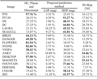
AVERAGE PREDICTION MODE USAGE ACROSS THE FOUR QPS, IN PERCENTAGE OF PIXELS, FOR THE HEVC-HOP-P CASE
Image DC, Planar and Directional Proposed prediction method SS-Skip [30] LOP stage HOP stage
PT0 57.76 % 3.32 % 22.81 % 16.12 % PT150 26.53 % 4.39 % 51.27 % 17.62 % DS 27.35 % 3.84 % 40.31 % 28.51 % DC 27.25 % 1.93 % 44.04 % 26.78 % LAURA 21.51 % 10.25 % 45.22 % 23.03 % SEAGULL 13.87 % 9.27 % 41.81 % 35.05 % BIKES 44.12 % 5.69 % 33.44 % 16.75 % DANGER 49.28 % 5.99 % 31.15 % 13.59 % FLOWERS 81.54 % 2.63 % 10.55 % 5.28 % STONE 82.66 % 2.75 % 9.60 % 4.99 % VESPA 38.42 % 7.94 % 30.03 % 23.61 % ANKY 24.39 % 10.89 % 30.26 % 34.46 % DESKTOP 57.50 % 2.67 % 15.68 % 24.14 % MAGNETS 28.88 % 9.57 % 28.42 % 33.14 % FOUNTAIN 30.12 % 8.38 % 37.66 % 23.84 % FRIENDS 78.01 % 3.08 % 11.35 % 7.57 % COLOR 15.62 % 8.94 % 38.14 % 37.30 % ISO 11.40 % 11.29 % 41.57 % 35.75 % TABLE III
BD-PSNR-Y AND BD-RATE RESULTS COMPARING HEVC,HEVC-SS(2DOF)
AND HEVC-HOP-P(8DOF) USING THE TESTING METHODOLOGY OF [23] Image
HEVC-SS vs HEVC HEVC-HOP-P vs HEVC-SS BD-PSNR-Y BD-RATE BD- PSNR-Y BD- RATE BIKES 0.78 dB -20.83 % 0.08 dB -2.41 % DANGER 0.57 dB -16.08 % 0.08 dB -2.41 % FLOWERS 0.17 dB -4.67 % 0.02 dB -0.69 % STONE 0.27 dB -8.43 % -0.03 dB 0.95 % VESPA 0.66 dB -32.79 % 0.09 dB -5.34 % ANKY 1.48 dB -62.57 % 0.11 dB -6.87 % DESKTOP 0.33 dB -15.23 % 0.10 dB -5.19 % MAGNETS 0.64 dB -37.90 % 0.08 dB -5.97 % FOUNTAIN 1.22 dB -35.38 % 0.12 dB -4.34 % FRIENDS 0.15 dB -10.40 % 0.03 dB -1.72 % COLOR 1.26 dB -58.40 % 0.18 dB -12.86 % ISO 1.49 dB -45.39 % 0.26 dB -10.81 % AVG. 0.75 dB -29.01 % 0.09 dB -4.81 % TABLE IV
CODEC COMPUTATIONAL COMPLEXITY COMPARISON
Encoder HEVC HEVC-SS HEVC-HOP-A HEVC-HOP-P HEVC-HOP-B Run time (h) 0.06 3.88 5.88 26.54 20.30 vs HEVC-SS 0.02 1 1.51 6.84 5.23 Decoder HEVC HEVC-SS HEVC-HOP-A HEVC-HOP-P HEVC-HOP-B Run time (s) 1.70 33.56 30.54 29.98 28.56 vs HEVC-SS 0.05 1 0.91 0.89 0.85 performance is evaluated using a Bjøntegaard Delta Metric. Additionally, several variants of HEVC-HOP are tested. These variants of HEVC-HOP are referred to as HEVC-HOP-A, HEVC-HOP-P and HEVC-HOP-B, respectively for Affine (six DoF), Projective (eight DoF) and Bilinear (eight DoF) GTs. Table I shows the RD performance comparison between HEVC and SS, and between SS and the various HEVC-HOP variants.
1) Comparison between LOP and HOP
Table I shows that HEVC-SS can outperform HEVC, for all tests, with bitrate savings up to 45.35%. Nevertheless, all versions of the proposed HEVC-HOP method are even more efficient than HEVC-SS to encode LF images. This increased
performance, with bitrate savings up to 12.62% for certain images relatively to HEVC-SS (49.82% relatively to HEVC), comes from the use of a higher order prediction model. Since HEVC-SS is limited to two DoF, it is not able to accurately describe block transformations more complex than a simple translation. When comparing the results by means of comparing the effectiveness of adding prediction tools with more than two DoF, it is possible to notice that for the encoded LF images, the best case is when eight DoF are used. If eight DoF are available, i.e., when HEVC-HOP-P is being used, four points of correspondence are transmitted, which allows the description of not only translations, but also rotations, scaling, shearing and perspective changes. In this case, although extra information needs to be encoded, relative to the HEVC-SS case, the bitrate savings increases to 5.86% (28.81% relative to HEVC), in average, for all tested LF images.
2) Comparison between the proposed GTs
The proposed prediction mode HEVC-HOP-B, using a Bilinear GT, can achieve similar results to HEVC-HOP-P for most images, both in terms of average PSNR (BD-PSNR) and bitrate savings. However, comparing the average performance of each method regarding the type of camera models (AVG. FOC and AVG. UNF) it is possible to observe that HEVC-HOP-P is slightly more efficient for the unfocussed model images and HEVC-HOP-B is slightly more efficient for the focused model images. In the case of HEVC-HOP-A only six DoF are available because only three points of correspondence are transmitted. When compared HOP-A to HEVC-HOP-P, the bitrate savings gains relatively to HEVC-SS are reduced to 4.84% (28.12% relatively to HEVC) on average considering all tested LF images, which may be due to the fact that HEVC-HOP-A is not able to compensate for perspective changes. However, in terms of computational complexity HOP-A is approximately 4.5 times faster than HEVC-HOP-P. Note that none of the implementations is optimized in terms of computational complexity; therefore, the reported values for comparison may vary. It is worthwhile mentioning that for some cases (e.g., STONE test image) HEVC-HOP-A can outperform both eight DoF GTs. In HEVC-HOP-P four correspondence points are always encoded, even if only three are necessary. Since in some cases, more information might be transmitted to describe the same GT, HEVC-HOP-P is, for this particular test image, less efficient than HEVC-HOP-A.
Regarding the computational complexity, a study was performed using the image VESPA, from the EPFL dataset of LF images. This image was encoded and decoded using the codecs, HEVC, HEVC-SS, HEVC-HOP-A, HEVC-HOP-P and HEVC-HOP-B, with QP=32. These tests were performed using a PC equipped with an Intel Xeon CPU E3-1240 [email protected] and 24GB of RAM, running Ubuntu 16.04. The obtained running time to encode and decode each image is depicted in Table IV. The computational complexity of the proposed schemes must be compared to HEVC-SS, as it is used as reference. The HEVC-SS complexity is equivalent to encoding a P-Slice in HEVC [30]. As can be seen from Table IV, the proposed algorithm increases the computational burden at the encoder side, where HEVC-HOP-A, HEVC-HOP-P and HEVC-HOP-B are 1.51, 6.84 and 5.23 times more complex than HEVC-SS, respectively. However, at the decoder the running time is reduced in relation to HEVC-SS. As the
IEEE Journal on Selected Topics in Signal Processing (JSTSP) - Special Issue on Light Field Image Processing 10
proposed method uses a more efficient prediction, the LF image encoder creates a lower number of partitions than the HEVC-SS.
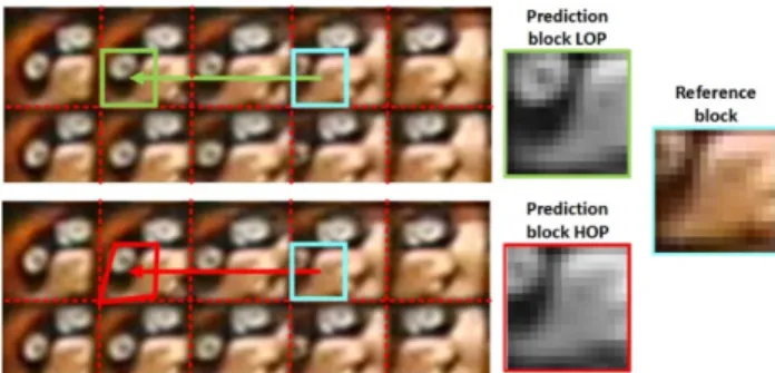
One of the most important advantages of the proposed prediction method is the ability to choose between the LOP stage and the HOP stage for each image block. This decision is taken based on RDO criteria, which allows the proposed HEVC-HOP to outperform HEVC-SS in all cases. In Table II it is possible to observe that despite the HOP stage of the proposed prediction method being used more frequently than the LOP stage, there is always a considerable part of the image that is encoded using only the LOP prediction mode. However, the fact that the HOP stage is used more often than the LOP stage alone indicates that, although the proposed method HEVC-HOP-P requires additional overhead for transmitting the prediction information, i.e., one flag (𝐹ghK) and four vectors (f𝑣⃗ghKij), it is very efficient in reducing the distortion between
the current block and prediction block, therefore reducing the RD cost. An example of this can be seen in Fig. 6 where a comparison between the generated prediction block using either the LOP method or the proposed HOP method is shown. As it is possible to see, the prediction block generated using the proposed HOP stage (𝐽ghK= 5080) is has a lower distortion when compared to the reference block than the prediction block using LOP (𝐽—hK= 7851). The parameters that describe the GT and that are transmitted to the decoder are the f𝑣⃗ghKij vectors, which in this specific case are {(3; 0), (4; 0), (2; −1), (2; 1)}. 3) Experimental results for rendered SAIs
To further evaluate the compression efficiency of the proposed HEVC-HOP-P, the objective quality of the SAIs extracted from the encoded LF images was tested. The experimental methodology adopted in [23] for the Lytro Illum unfocused camera setup was used. In this case, the PSNR-Y is calculated as an average of the PSNR-Y of 13×13 SAIs. This average PSNR-Y compares reference and reconstructed (i.e., encoded and decoded) SAIs. The processing chain designed to generate the SAIs consists in converting the hexagonal lenslet LF image to a square lenslet LF image (with 15x15 pixels per MI) and then, extracting one pixel, in a fixed position from each square MI, to render each SAI. For this case only the images from [23] have been used. The only difference to the methodology in [23] is that, instead of using fixed compression ratios, the results are calculated using the reconstructed images attained with fixed QPs (22, 27, 32 and 37), i.e., the number of bits is the same as in the previously used methodology.
From the results presented in Table III it is possible to observe that there is a coherence between the results for the
encoded LF images and the rendered SAIs. The average bitrate savings achieved by HEVC-HOP-P relative to HEVC-SS are very similar for both cases. Nevertheless, as the RD cost was not optimized on each SAI, the results are not exactly the same. As previously explained, when using the HEVC-HOP-P method the LF image is encoded “as is”, without the need to know any information about the used lenslet based LF camera. This may explain the bitrate increase for image STONE, as the proposed method calculates the RD cost based on the lenslet LF image, instead of the generated view or SAI.
Additionally, a comparison between the proposed HEVC-HOP-P and the state-of-the-art method [24] was performed. In [24], a comparison in relation to JPEG, using the EPFL dataset, reports a gain of 4.54 dB in the BD-PSNR. Similarly, this image set were encoded by the proposed HEVC-HOP-P, with QPs {22, 27, 32, 37}, achieving a BD-PSNR gain of 4.83 dB, in relation to JPEG. For a wider QP range {17, 22, 27, 32, 37}, the gain of HEVC-HOP-P decreases to 4.34 dB. Thus, it is fair to assume that the proposed HEVC-HOP-P has a very similar performance to the state-of-the-art method [24].
4) Results for different lenslet LF camera models
In general, the bitrate savings across the different codecs when compared to HEVC are higher when encoding LF images captured with cameras using a focused LF camera model. This is possible to see when comparing the average bitrate savings for the LF images captured with an unfocused camera model or the focused camera model in Table II. This occurs because HEVC-SS and HEVC-HOP are based on matching prediction tools. In the focused images, the MIs are focused, therefore sharper than the unfocussed images. In sharper MI, more prominent features exist and therefore the block matching is more reliable [34]. Additionally, since the incident light in the camera’s sensor in the unfocused case is focused at infinity, the disparity between MIs tends to be zero, which means that theoretically no perspective compensation can be matched. This can be justified by the noticeable lower relative prediction mode usage, shown in Table II, for the proposed prediction method as well as SS-Skip for most LF images captured with unfocused camera models.
The proposed HOP model is also more suited to adapt to non-rectangular shape MIs, e.g., hexagonal and circular shape, when compared to LOP model based methods. This happens because the corners of the prediction blocks, when using the proposed HOP model, are flexible to adapt for different block shapes.
VI. CONCLUSIONS
In this paper, a HOP mode for LF image coding was proposed, using geometric transformations of up to eight DoF. The proposed HOP mode is a two-stage block-wise approach that is able to achieve RD efficiency gains, relative to a LOP state-of-the-art solution for LF image coding and HEVC. These gains occur, regardless of the LF camera model, MI and LF image resolution and microlens array type. Experimental results show average bitrate savings of 5.86% and 28.81%, when compared to a LOP state-of-the-art solution and HEVC, respectively, across different types of LF images, when using the Projective GT. It is also possible to conclude that, the GTs with eight DoF, namely Projective and Bilinear, are generally more efficient than Affine GT in a RD sense.
Fig. 6 - Comparison between the prediction block generated by LOP and HOP stages.
IEEE Journal on Selected Topics in Signal Processing (JSTSP) - Special Issue on Light Field Image Processing 11 An additional testing methodology, based on the SAI
objective quality, was also used to confirm the bitrate savings when comparing HOP with LOP tools. In this case the average bitrate savings achieved is 4.81% and 31.77% when comparing the HOP mode with the state-of-the-art LOP solution and HEVC, respectively.
Future work will include the investigation of GT parameter prediction techniques and optimal HOP model selection, aiming to combine them in the same codec. Additionally, entropy encoding improvements will also be considered, namely, the binarization of the HOP model vectors.
REFERENCES
[1] T. Georgiev and A. Lumsdaine, “Rich Image Capture with Plenoptic Cameras,” in Proc. IEEE Inter. Conf. on Computational Photography, Cluj-Napoca, Romania, 2010, pp. 1–8.
[2] J. Arai, “Integral three-dimensional television (FTV Seminar),” Sapporo, Japan, ISO/IEC JTC1/SC29/WG11 MPEG2014/N14552, Jul. 2014.
[3] X. Xiao, B. Javidi, M. Martinez-Corral, and A. Stern, “Advances in Proc. three-dimensional integral imaging: sensing, display, and applications,” Appl. Opt., vol. 52, no. 4, pp. 546–560, Feb. 2013. [4] A. Lumsdaine and T. Georgiev, “The focused plenoptic camera,” in
Proc. IEEE Inter. Conf. Computational Photography, 2009, pp. 1–8. [5] C. Hahne, A. Aggoun, S. Haxha, V. Velisavljevic, and J. C. J.
Fernández, “Light field geometry of a standard plenoptic camera,” Opt. Express, vol. 22, no. 22, pp. 26659–26673, Nov. 2014.
[6] “JPEG PLENO Abstract and Executive Summary,” Sydney, ISO/IEC JTC 1/SC 29/WG1 N6922, Feb. 2015.
[7] S. Kumar and R. C. Jain, “Low complexity fractal-based image compression technique,” IEEE Trans. on Consumer Electronics, vol. 43, no. 4, pp. 987–993, Nov. 1997.
[8] H. Huang, J. W. Woods, Y. Zhao, and H. Bai, “Control-Point Representation and Differential Coding Affine-Motion Compensation,” IEEE Trans. on Circuits and Systems for Video Technology, vol. 23, no. 10, pp. 1651–1660, Oct. 2013.
[9] T. Wiegand, E. Steinbach, and B. Girod, “Affine multipicture motion-compensated prediction,” IEEE Trans. on Circuits and Systems for Video Technology, vol. 15, no. 2, pp. 197–209, Feb. 2005.
[10] M. Tok, M. Esche, A. Glantz, A. Krutz, and T. Sikora, “A Parametric Merge Candidate for High Efficiency Video Coding,” in Proc. Data Compression Conf., 2013, pp. 33–42.
[11] A. Krutz, A. Glantz, M. Tok, M. Esche, and T. Sikora, “Adaptive Global Motion Temporal Filtering for High Efficiency Video Coding,” IEEE Trans. on Circuits and Systems for Video Technology, vol. 22, no. 12, pp. 1802–1812, Dec. 2012.
[12] M. Tok, A. Glantz, A. Krutz, and T. Sikora, “Feature-based global motion estimation using the Helmholtz principle,” in Proc. IEEE Inter. Conf. Acoustics, Speech and Signal Processing, 2011, pp. 1561–1564. [13] R. C. Kordasiewicz, M. D. Gallant, and S. Shirani, “Affine Motion Prediction Based on Translational Motion Vectors,” IEEE Trans. on Circuits and Systems for Video Technology, vol. 17, no. 10, pp. 1388– 1394, Oct. 2007.
[14] X. San, H. Cai, J. G. Lou, and J. Li, “Multiview Image Coding Based on Geometric Prediction,” IEEE Trans. on Circuits and Systems for Video Technology, vol. 17, no. 11, pp. 1536–1548, Nov. 2007. [15] K. Müller et al., “3D High-Efficiency Video Coding for Multi-View
Video and Depth Data,” IEEE Trans. on Image Processing, vol. 22, no. 9, pp. 3366–3378, Sep. 2013.
[16] R. J. S. Monteiro, N. M. M. Rodrigues, and S. M. M. Faria, “Disparity compensation using geometric transforms,” in Proc. 3DTV-Conf.: The True Vision - Capture, Transmission and Display of 3D Video, 2014, pp. 1–4.
[17] R. J. S. Monteiro, N. M. M. Rodrigues, and S. M. M. Faria, “Geometric transforms and reference picture list optimization for efficient disparity compensation,” in Proc. Inter. Conf. on Image Processing Theory, Tools and Applications, 2015, pp. 370–375.
[18] A. Aggoun, “A 3D DCT Compression Algorithm For Omnidirectional Integral Images,” in Proc. IEEE Inter. Conf. on Acoustics, Speech and Signal Processing, 2006, vol. 2, pp. II–II.
[19] M. C. Forman and A. Aggoun, “Quantisation strategies for 3D-DCT-based compression of full parallax 3D images,” in Proc. Inter. Conf. on Image Processing and Its Applications, 1997, vol. 1, pp. 32–35. [20] A. Aggoun, “Compression of 3D Integral Images Using 3D Wavelet
Transform,” Journal of Display Technology, vol. 7, no. 11, pp. 586– 592, Nov. 2011.
[21] F. Dai, J. Zhang, Y. Ma, and Y. Zhang, “Lenselet image compression scheme based on subaperture images streaming,” in Proc. IEEE Inter. Conf. on Image Processing, 2015, pp. 4733–4737.
[22] A. Vieira, H. Duarte, C. Perra, L. Tavora, and P. Assuncao, “Data formats for high efficiency coding of Lytro-Illum light fields,” in Proc. Inter. Conf. on Image Processing Theory, Tools and Applications, 2015, pp. 494–497.
[23] “ICME 2016 Grand Challenge: Light-Field Image Compression.” [Online]. Available: http://mmspg.epfl.ch/files/content/sites/mmspl/ files/shared/LF-GC/CFP.pdf. [Accessed: 01-Dec-2016].
[24] D. Liu, L. Wang, L. Li, Z. Xiong, F. Wu, and W. Zeng, “Pseudo-sequence-based light field image compression,” in Proc. IEEE Inter. Conf. on Multimedia Expo Workshops, 2016, pp. 1–4.
[25] J. B. Jianle Chen Elena Alshina, Gary J.Sullivan, Jens-Rainer Ohm, “Algorithm description of Joint Exploration Test Model 3 (JEM3), ISO/IEC JTC1/SC29/WG11/N16276,” Jun. 2016.
[26] M. Magnor and B. Girod, “Data compression for light-field rendering,” IEEE Trans. on Circuits and Systems for Video Technology, vol. 10, no. 3, pp. 338–343, Apr. 2000.
[27] B. Girod, C.-L. Chang, P. Ramanathan, and X. Zhu, “Light field compression using disparity-compensated lifting,” in Proc. Inter. Conf. on Multimedia and Expo, 2003, vol. 1, p. I-373-6.
[28] Y. Li, M. Sjöström, and R. Olsson, “Coding of plenoptic images by using a sparse set and disparities,” in IEEE Inter. Conf. on Multimedia and Expo, 2015, pp. 1–6.
[29] Y. Li, M. Sjöström, R. Olsson, and U. Jennehag, “Scalable Coding of Plenoptic Images by Using a Sparse Set and Disparities,” IEEE Trans. on Image Processing, vol. 25, no. 1, pp. 80–91, Jan. 2016.
[30] C. Conti, L. D. Soares, and P. Nunes, “HEVC-based 3D holoscopic video coding using self-similarity compensated prediction,” Signal Processing: Image Communication, vol. 42, pp. 59–78, Mar. 2016. [31] C. Conti, P. Nunes, and L. D. Soares, “HEVC-based light field image
coding with bi-predicted self-similarity compensation,” in Proc. IEEE Inter. Conf. on Multimedia Expo Workshops, 2016, pp. 1–4.
[32] L. F. R. Lucas et al., “Locally linear embedding-based prediction for 3D holoscopic image coding using HEVC,” in European Signal Processing Conf., Lisbon, Portugal, 2014, pp. 11–15.
[33] Y. Li, M. Sjöström, R. Olsson, and U. Jennehag, “Coding of Focused Plenoptic Contents by Displacement Intra Prediction,” IEEE Trans. on Circuits and Systems for Video Technology, vol. 26, no. 7, pp. 1308– 1319, Jul. 2016.
[34] Y. Li, R. Olsson, and M. Sjöström, “Compression of unfocused plenoptic images using a displacement intra prediction,” in Proc. IEEE Inter. Conf. on Multimedia Expo Workshops, 2016, pp. 1–4.
[35] R. I. Hartley and A. Zisserman, Multiple View Geometry in Computer Vision, Second. Cambridge University Press, 2004.
[36] P. S. Heckbert, “Fundamentals of Texture Mapping and Image Warping,” EECS Department, University of California, Berkeley, UCB/CSD-89-516, Jun. 1989.
[37] J. Jain and A. Jain, “Displacement Measurement and Its Application in Interframe Image Coding,” IEEE Trans. on Communications, vol. 29, no. 12, pp. 1799–1808, Dec. 1981.
[38] C.-H. Cheung and L.-M. Po, “A novel cross-diamond search algorithm for fast block motion estimation,” IEEE Trans. on Circuits and Systems for Video Technology, vol. 12, no. 12, pp. 1168–1177, Dec. 2002. [39] J. R. Ohm, G. J. Sullivan, H. Schwarz, T. K. Tan, and T. Wiegand,
“Comparison of the Coding Efficiency of Video Coding Standards - Including High Efficiency Video Coding (HEVC),” IEEE Trans. on Circuits and Systems for Video Technology, vol. 22, no. 12, pp. 1669– 1684, Dec. 2012.
[40] F. Bossen, B. Bross, K. Suhring, and D. Flynn, “HEVC Complexity and Implementation Analysis,” IEEE Trans. on Circuits and Systems for Video Technology, vol. 22, no. 12, pp. 1685–1696, Dec. 2012. [41] A. Agooun, et al, “Acquisition, processing and coding of 3D holoscopic
content for immersive video systems,” in Proc. 3DTV-Conf.: The True Vision-Capture, Transmission and Dispaly of 3D Video, Aberdeen, 2013, pp. 1–4.
[42] G. Todor, “Gallery and Lightfield Data.” [Online]. Available: http://www.tgeorgiev.net/Gallery/. [Accessed: 01-Dec-2016].