Repositório ISCTE-IUL
Deposited in Repositório ISCTE-IUL: 2018-10-12
Deposited version: Post-print
Peer-review status of attached file: Peer-reviewed
Citation for published item:
Strobbe, T, Eloy, S., Pauwels, P., Verstraeten, R., De Meyer, R. & Campenhout, J. V. (2016). A graph-theoretic implementation of the Rabo-de-Bacalhau transformation grammar. Artificial Intelligence for Engineering Design, Analysis and Manufacturing. 30 (2), 138-158
Further information on publisher's website: 10.1017/S0890060416000032
Publisher's copyright statement:
This is the peer reviewed version of the following article: Strobbe, T, Eloy, S., Pauwels, P.,
Verstraeten, R., De Meyer, R. & Campenhout, J. V. (2016). A graph-theoretic implementation of the Rabo-de-Bacalhau transformation grammar. Artificial Intelligence for Engineering Design, Analysis and Manufacturing. 30 (2), 138-158, which has been published in final form at
https://dx.doi.org/10.1017/S0890060416000032. This article may be used for non-commercial purposes in accordance with the Publisher's Terms and Conditions for self-archiving.
Use policy
Creative Commons CC BY 4.0
The full-text may be used and/or reproduced, and given to third parties in any format or medium, without prior permission or charge, for personal research or study, educational, or not-for-profit purposes provided that:
• a full bibliographic reference is made to the original source • a link is made to the metadata record in the Repository • the full-text is not changed in any way
The full-text must not be sold in any format or medium without the formal permission of the copyright holders. Serviços de Informação e Documentação, Instituto Universitário de Lisboa (ISCTE-IUL)
Av. das Forças Armadas, Edifício II, 1649-026 Lisboa Portugal Phone: +(351) 217 903 024 | e-mail: [email protected]
1
A graph-theoretic implementation of the Rabo-de-Bacalhau transformation
grammar
Tiemen Strobbe a,*, Sara Eloy b, Pieter Pauwels a, Ruben Verstraeten a, Ronald De Meyer a, Jan Van Campenhout c
a
Department of Architecture and Urban Planning, Ghent University, J. Plateaustraat 22, 9000 Ghent, Belgium.
b
Department of Architecture and Urbanism, Instituto Universitário de Lisboa (ISCTE-IUL, ISTAR-IUL), Av. das Foras Armadas 1649-026, Lisbon, Portugal.
c
Department of Electronics and Information Systems, Ghent University, Sint-Pietersnieuwstraat 41, 9000 Ghent, Belgium.
*
Corresponding author, J. Plateaustraat 22, 9000 Ghent, Tel +32 9 264 3880, [email protected]
Short title: Graph-theoretic shape grammar implementation
Number of pages: 49
Number of tables: 2
2
A graph-theoretic implementation of the Rabo-de-Bacalhau transformation
grammar
Abstract:
Shape grammars are rule-based formalisms for the specification of shape languages. Most of the existing shape grammars are developed on paper and have not been implemented computationally, so far. Nevertheless, the computer implementation of shape grammar is an important research question, not only to automate design analysis and generation, but also to extend the impact of shape grammars towards design practice and computer-aided design tools. In this paper, we investigate the implementation of shape grammars on a computer system, using a graph-theoretic representation. In particular, we describe and evaluate the implementation of the existing Rabo-de-Bacalhau transformation grammar. A practical step-by-step approach is presented, together with a discussion of important findings noticed during the implementation and evaluation. The proposed approach is shown to be both feasible and valuable in several aspects; We show how the attempt to implement a grammar on a computer system leads to a deeper understanding of that grammar, and might result in the further development of the grammar; We show how the proposed approach is embedded within a commercial CAD environment to make the shape grammar formalism more accessible to students and practitioners, thereby increasing the impact of grammars on design practice; and the proposed step-by-step implementation approach has shown to be feasible for the implementation of the Rabo-de-Bacalhau transformation grammar, but can also be generalized using different ontologies for the implementation.
Keywords:
3
1. Introduction
1
Spatial grammars are rule-based, generative and visual formalisms for the specification of spatial
2
languages. Spatial grammars include set grammars, graph grammars, shape grammars, and other kinds
3
of grammars for describing spatial languages. This ‘uniform treatment’ of grammars is introduced in the
4
work of Krishnamurti & Stouffs (1993), and also used in later work of Hoisl & Shea (2011) and McKay et
5
al. (2012). The potential of shape grammars (a specific kind of spatial grammar) as a theoretical
6
framework for analyzing and generating (architectural) designs has been demonstrated through a broad
7
range of formal studies (Koning & Eizenberg, 1981; Duarte, 2005; Flemming, 1987; Stiny, 1977).
8
However, many existing grammars in architectural design (and other design disciplines) are developed
9
on paper, and relatively few grammars have been implemented computationally, so far. Some
10
exceptions can be found, including the work of Aksamija et al. (2010), Granadeiro et al. (2013), and Grasl
11
(2012). Nevertheless, the computer implementation of shape grammars remains an open research
12
question, because there seems to be no definite answer in the literature on how shape grammars can be
13
implemented to a computer system. For example, a recent overview of McKay et al. (2012) summarizes
14
the key limitations, benefits, and open challenges of the main representative shape grammar
15
implementations to date. The question how to implement shape grammars is also an important research
16
question, because computer implementations are beneficial in many cases, including: to automate
17
several aspects of design analysis and generation (especially for grammars that are too extensive to
18
explore manually), to learn from the computer implementation about the design of the shape grammar
19
itself, and to extend the impact of shape grammars towards design practice and computer-aided-design
20
tools by providing tools to apply shape grammars in practice.
21
In this paper, we describe a method for the implementation of a shape grammar, originally developed on
22
paper, on a computer system using a graph-theoretic representation of this grammar. We start from a
4
literature review of previous research efforts in which spatial grammars are implemented to a computer
24
system (Section 2). In particular, the definition and characteristics of different kinds of spatial grammars
25
are compared, thereby focusing on shape grammars since they are often used for analyzing and
26
synthesizing architectural and creative designs. Also, an overview of previous shape grammar
27
implementation approaches is given. Next, we describe the research method, in which we point out a
28
practical step-by-step approach for the computer implementation of shape grammars (Section 3). In the
29
following section (Section 4), the proposed approach is evaluated through the implementation of the
30
Rabo-de-Bacalhau (RdB) transformation grammar, originally developed by Eloy (2012). In particular,
31
three relevant types of rules that are used in the RdB transformation grammar are implemented: (1)
32
assignment rules, (2) rules to connect spaces by eliminating walls, and (3) rules to divide spaces by
33
adding walls. A discussion of several issues encountered during the implementation and an evaluation of
34
the proposed approach is given in Section 5. Finally, conclusions and future research are described in
35
Section 6.
36
The work presented in this paper contributes to the current state of the art in shape grammar
37
implementations in several ways. First and foremost, a practical step-by-step approach is presented for
38
the computer implementation of a shape grammar. While the proposed approach builds further on
39
existing research on the graph-theoretic representation of shapes, such as recent work of Grasl (2013)
40
and Wortmann (2013), the proposed approach is also different because it can be applied in different
41
contexts, ranging from simple shape grammars to more complex grammars. Second, the implementation
42
of the RdB transformation grammar (Eloy, 2012) is in itself a useful contribution, because it
43
demonstrates how shape grammar implementations can be applied in architectural design practice. In
44
most papers on shape grammar implementations, the approach is validated through a rather
45
straightforward “showcase” grammar, while the RdB transformation grammar is more complex due to
46
the parallel representation of designs, rule conditions, etc., but it is also an example of a grammar that is
5
being used in practice. One of the most common criticisms to shape grammars is that there is little
48
evidence of their use in practice, so the implemented RdB transformation grammar serves as an example
49
application in architectural design practice, in particular, the development of a (semi)automated
50
methodology for supporting mass housing refurbishment. Third, the case study of implementing the
51
existing RdB transformation grammar reveals several findings on how grammar designers can learn from
52
the implementation about the design of the original grammar, and about the implications on the original
53
grammar itself. Finally, the proposed approach is embedded within a commercial computer-aided design
54
(CAD) environment to make the shape grammar formalism more accessible to students and practitioners
55
(architects, product designers), and therefore, it might increase the impact of shape grammars on design
56
practice.
57
2. Related work
58
In this section, we compare the definition and characteristics of different kinds of spatial grammars. In
59
particular, we focus on shape grammars since they are often used for analyzing and synthesizing
60
architectural and creative designs. Also, we provide a literature review of previous research efforts in
61
which a graph formalism is used for shape grammar implementations.
62
2.1.
Spatial grammars
63
Grammars, in general, are formal mathematical structures for specifying languages. All different kinds of
64
grammars (string grammars, shape grammars, graph grammars, and set grammars) share certain
65
definitions and characteristics (Krishnamurti & Stouffs, 1993). In particular, a grammar is defined as a
4-66
tuple (N, T, R, I) where:
67
N is a finite set of non-terminal entities;
68
T is a finite set of terminal entities;
6 R is a finite set of rewriting rules or productions;
70
I is an initial entity, a subset of N ∪ T.
71
A rewriting rule (or production) has the form lhs → rhs and can be considered as an “IF-THEN”
72
statement. The left hand side (lhs) contains entities from T and N, but cannot be empty. The right hand
73
side (rhs) also contains entities from T and N, but can be empty. A rule can be applied if the left hand
74
side of the rule matches a part of the given object, under a certain transformation (f). If this is the case,
75
the matching part of the given object is replaced by the right hand side of the rule, under the same
76
transformation f. As a result, a grammar defines a language that contains all objects generated by this
77
grammar.
78
Spatial grammars, in particular, are specific kinds of grammars that operate on objects in an Euclidean
79
space E² (for two-dimensional objects) or E³ (for three-dimensional objects). Krishnamurti and Stouffs
80
(1993) describe four kinds of grammars that can serve as spatial grammars: string grammars, set
81
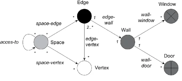
grammars, graph grammars and shape grammars. String grammars deal with a single string of symbols,
82
in which each symbol corresponds to a geometrical entity represented as a graphical icon. Set grammars
83
deal with spatial objects that are described as sets of geometrical entities. For example,
three-84
dimensional solids can be represented as collections of faces, edges and vertices. An example that
85
combines string and set grammars can be found in the work of Woodbury et al. (1992). Graph grammars
86
deal with a set of entities (nodes) where some pairs of entities are connected by links (edges). A common
87
characteristic of string grammars, set grammars and graph grammars is that spatial objects are
88
represented using symbolic entities: strings, sets and graphs, respectively.
89
Unlike other spatial grammars, shape grammars operate directly on spatial objects (shapes), rather than
90
through symbolic entities (Stiny, 2006). A powerful feature of shape grammars is that shapes and their
7
properties can be reinterpreted continuously during the process of rule application, allowing emergence
92
of shape features or properties that are not apparent in the initial definition of the shapes (Knight, 2003).
93
In shape grammar theory, algebras are used to represent shapes. An algebra Uij consists of a set of
94
geometrical shapes defined in dimension i = 0, 1, 2 or 3, which are points, lines, planes and solids,
95
respectively. These shapes are combined in a dimension j ≥ i. Also, labels and weights are introduced to
96
define new algebras Vij and Wij (Stiny, 1991).
97
In the architectural design domain, shape grammars are often used for analyzing and generating creative
98
designs (Koning & Eizenberg, 1981; Duarte, 2005; Flemming, 1987; Stiny, 1977). Relatively few of such
99
shape grammars have been implemented to a computer system, with some exceptions available
100
(Aksamija et al., 2010; Grasl, 2012; Granadeiro et al., 2013). Typically, the user of such unimplemented
101
shape grammars is meant to interpret the grammar and manually apply the rules in order to generate
102
designs (see the work of Chase (2002) for an overview of interaction strategies with shape grammars).
103
For computer implementations of shape grammars, on the other hand, the computer system should
104
automatically determine where and how rules are to be applied. While human designers are extremely
105
good at recognizing possible rule applications and readily make meaning from visual fragments, there is
106
general agreement that the ability of computer systems for shape recognition and interpretation is
107
below human capacities. For example, Jowers (2010) has successfully applied automatic object
108
recognition techniques (in particular, a method called Hausdorff distance) to interpret shapes without an
109
underlying representation. However, this implementation is also limited; for example, it may not be able
110
to identify spaces in a floor plan, while a (trained) human person can almost immediately detect
111
different spaces by just looking at the floor plan. While computer systems often rely on predefined
112
representations in order to interpret given information, shape grammars rely on emergence and
113
continuously changing representations, thus making them not particularly amenable for computer
114
implementation. Even for shape grammars that do not support emergence, the detection of applicable
8
rules is a complex task to solve for computer, such as finding subshapes for rule application
116
(Krishnamurti, 1981).
117
A large spectrum of shape grammar types can be identified (Knight, 1999; Yue & Krishnamurti, 2014),
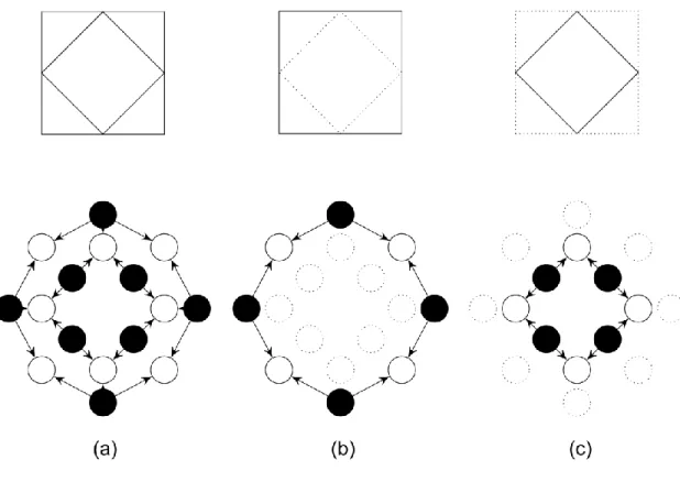
118
including subshape-driven versus label-driven shape grammars, nonparametric versus parametric shape
119
grammars, rectilinear versus curvilinear shape grammars, and shape grammars with or without
120
emergence enabled. As Yue & Krishnamurti (2014) point out, the complexity and choice of the
121
implementation approach depends on the type of shape grammar to be implemented. In this paper, we
122
propose an implementation approach that consists of translating a shape grammar to a graph-theoretic
123
equivalent grammar. Graphs provide an elegant way to describe topological compositions and incidence
124
relations of spatial objects, but can also account for geometrical properties by associating attributes to
125
the graph objects. Moreover, practical solutions and algorithms for (sub)graph matching and automatic
126
rule application exist in the literature (Geiβ et al., 2006; Taentzer, 2004). This graph-based approach is
127
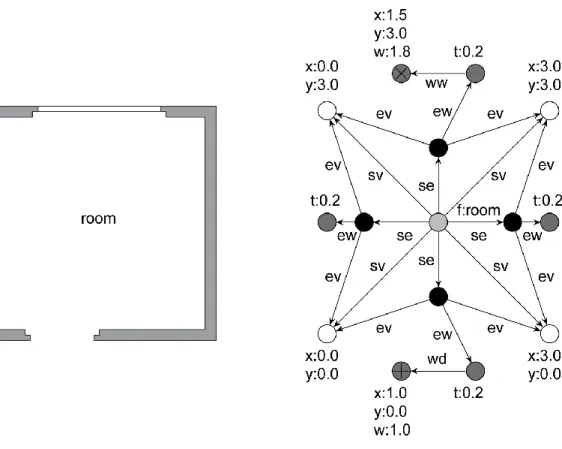
applicable for shape grammars that are either subshape-driven or label-driven and support parametric
128
shapes. Another important benefit of using such a graph-based implementation approach is that shape
129
grammars can also be implemented with emergence enabled. A short discussion of this can be found in
130
Section 3.1 and other research work of Grasl (2013) and Wortmann (2013), however, enabling
131
emergence is not the main topic of this paper. An aspect that is not considered in this paper is how to
132
support curvilinear shapes, but a good discussion of this can be found in the work of Jowers & Earl
133
(2011). An overview of existing shape grammar implementations, including graph-based approaches and
134
other approaches, is presented in the following section.
9
2.2.
Previous implementation approaches
136
The implementation of shape grammars has been the subject of many research efforts since the original
137
conception of shape grammars in the 1970s (Stiny & Gips, 1971). The dilemma, addressed by Gips
138
(1999), is the tension between the visual nature of shape grammars and the inherently symbolic nature
139
of computer representations and processing. An overview of more recent research efforts is given in the
140
work of Gips (1999 and Chase (2010). Chase (2010) summarizes the main representative shape grammar
141
implementation systems (Li et al., 2009; Trescak et al., 2012; Hoisl & Shea, 2011; Jowers & Earl, 2011;
142
Ertelt & Shea, 2010; Correia et al., 2010). These systems are analyzed and compared in terms of form,
143
semantics, definition interface and generative capabilities. McKay et al. (2012) analyze these systems
144
according to four characteristics: representation and algorithms, user interaction and interface, support
145
for particular problems, support for specific stages of the development process. Currently available
146
implementations, although still prototypes and each focusing on just a few particular aspects, have made
147
valuable contributions on enabling subshape recognition, emergence, parametric rules, curvilinear
148
shapes, and present more user friendly interfaces and flexible representation processes.
149
A fundamentally different approach towards shape grammar implementation is the use of graphs as an
150
underlying framework for representing shapes. Graphs are data structures that represent a set of
151
entities (nodes) where some pairs of entities are connected by links (edges). Graphs offer a natural
152
framework to model spatial entities (solids, faces, edges, and vertices) and the relations between these
153
entities. The use of graphs to represent spatial shapes or designs is not uncommon in the architectural
154
design domain. For example, Fitzhorn (1990) uses graphs to represent three-dimensional solids and
155
Steadman (1976) describes a graph-theoretic representation of architectural arrangements. If graphs are
156
used to represent shapes or designs, graph rewriting systems can be used to create new graphs out of an
157
original graph, similarly to how it occurs for shape grammars. Graph grammars are used for divergent
10
purposes, but they can also be used to develop formal languages of spatial objects. Among the first
159
attempts to describe such formal languages is the approach of Fitzhorn (1990). In this approach, a graph
160
grammar is defined to generate boundary representations of three-dimensional solids. These solids are
161
defined as sets of geometrical entities (solid, face, edge and vertex) and their corresponding topological
162
relations. The production rules of the grammar are defined as Euler operators in order to generate solids
163
that are syntactically correct. This approach was adopted and extended in the work of Heisserman
164
(1994). In this approach, three-dimensional solids are represented as labeled boundary graphs, and
165
boundary solid grammars are used to develop spatial languages. Other examples include the work of
166
Shea & Cagan (1999), in which graph-like shapes are applied to produce structural forms, and the work
167
of Helms & Shea (2012) on representing designs as graphs. In other recent work, it has been
168
demonstrated how graph grammars can also represent parametric shape grammars, and how
169
emergence, a foundational feature of shape grammars, can be supported (Grasl, 2013; Wortmann,
170
2013). In recent work of Grasl & Economou (2013), a graph-based shape grammar library called GRAPE is
171
proposed that provides a general framework for graph-based shape grammar implementations.
172
In conclusion, several shape grammar implementation systems are available, each having a specific focus
173
and purpose. The shared focus of these systems is to allow designers or shape grammar users to
174
implement their shape grammar on a computer system. Still, computer implementations of complex
175
shape grammars are seldom. An interesting counterexample can be found in the work of Grasl (2012), in
176
which a graph-theoretic equivalent of the Palladian shape grammar is described that can generate the
177
same language of Palladian villas as the original shape grammar introduced by Stiny & Mitchell(1978). In
178
the next section, an approach for the implementation of shape grammars is proposed that, on the one
179
hand, builds further on existing research on the graph-theoretic representation of shapes and shape
180
grammars (Grasl, 2013; Wortmann, 2013), but it is also more general than previous approaches and it
181
can be applied in different contexts.
11
3. Method: Implementing a shape grammar
183
In order to translate a shape grammar, specified on paper, to a computer-amenable and graph-theoretic
184
grammar, several steps are needed. In this section, a step-by-step approach is given to define a
graph-185
theoretic representation of the shape grammar to be implemented.
186
3.1.
Step 1: Defining the ontology
187
The first step in the proposed translation of a shape grammar to a graph-theoretic grammar is to
188
construct an ontology that defines the node types, node properties and relations between the nodes. A
189
graph is a mathematical structure that represents relations between nodes. Therefore, the node types
190
that are used and the possible relations between different node types of the graph-theoretic grammar
191
must be defined. In other words, this corresponds to defining an ontology beforehand, which allows
192
computers to more easily interpret given visual information in terms of this predefined ontology. The
193
predefined ontology should describe the different entities considered and how they relate to other
194
entities (spaces, walls, edges, vertices, and other kinds of geometric, semantical, or spatial entities). This
195
ontology determines what information can be expressed in the computerized grammar and how this
196
information will be interpreted by the computer system. The definition of an ontology depends on the
197
given shape grammar and on the envisioned functionality of the grammar implementation; for example,
198
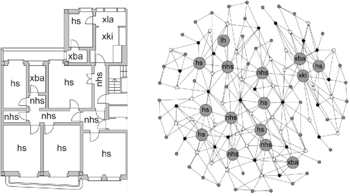
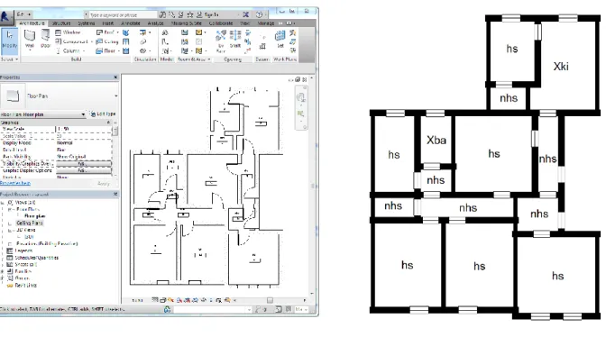
if the given shape grammar concerns only two-dimensional shapes, the ontology needed is more limited
199
than for shape grammars that operate with more complex semantic entities (such as walls, spaces, and
200
other architectural concepts).
201
As an example, an ontology with six different node types is considered: vertex, edge, space, wall, door,
202
and window. With such an ontology, the computer system is able to recognize both geometrical entities
203
(vertex and edge) and non-geometrical entities (space, wall, door and window. Also, seven different
204
relations between the predefined node types are defined: vertex, space-edge, space-vertex,
12
wall, wall-door, wall-window, and access-to. In the domain of graph grammars, a type graph provides a
206
useful way to represent which node types are allowed and which edge types can be used to define
207
relations between the nodes (which is exactly the ontology). Figure 1 shows the type graph for the six
208
node types and seven edge types. Both geometrical and non-geometrical node types are shown as
209
circles, using different colors to indicate the different types. The multiplicity of a node type specifies the
210
number of other nodes (using a lower and upper bound) that can be connected to this node, using a
211
given edge type. Depending on whether the multiplicity is defined at the end or source of the edge type,
212
this defines the number of incoming or outgoing edges, respectively. If an indefinite number of
213
connections is allowed, this is indicated using an asterisk (*).
214
Figure 1: The type graph defines the node and edge types used for the grammar implementation.
If an indefinite number of nodes or connections is allowed between node and edge types, this is
indicated using an asterisk (*).
For unimplemented shape grammars (developed on paper), architectural designs and objects (spaces,
215
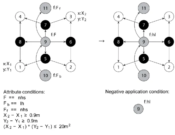
walls, doors, and windows) are all represented as shapes. The power of these shape grammars lies in the
216
fact that shapes and their properties can be reinterpreted continuously (Stiny, 2006), allowing the
217
emergence of features which are not apparent in the initial definition of a shape. For a good theoretical
13
overview of emergence in shape grammars, we refer to the work of Knight (2003). Using a graph-based
219
ontology to implement a grammar, shapes are now considered in terms of finite sets of entities, relations
220
between these entities, and entity properties. One of the main advantages is that computer systems are
221
now able to ‘interpret’ the visual information using the underlying graph representation. For many
222
simple shape grammars, an ontology that contains only geometrical node types (vertex, edge) would be
223
sufficient. Moreover, in the work of Grasl (2013) and Wortmann (2013) it is shown that when shapes are
224
represented as graphs with geometrical nodes, the characteristic features of shapes (emergence and
225
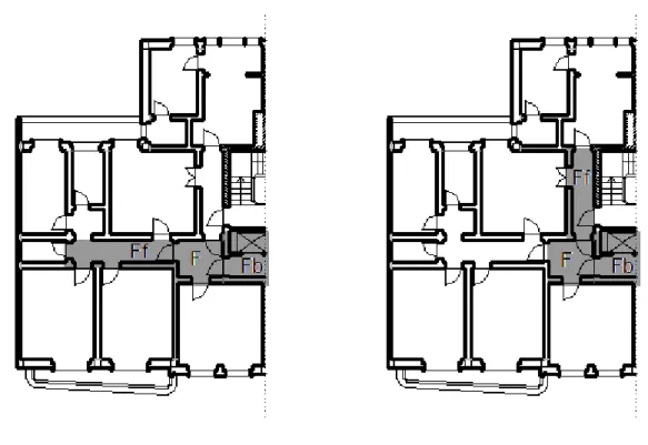
reinterpretation of shapes) can be maintained. In particular, GRAPE (Grasl, 2013) is a shape grammar
226
implementation system in which shape emergence is supported by continuously translating graphs to
227
shapes, and Wortmann (2013) describes several algorithms to translate simple two-dimensional shapes
228
in the algebra U12 to graphs. In other words, none of the essential features of shapes are lost when
229
translating shapes to this kind of graphs. While (architectural) designs can be represented as (collections
230
of) shapes, and thus be translated to graphs with only geometrical nodes, this would result in very large
231
graphs, especially when a lot of semantic elements or details are involved.
232
In order to avoid overly large graphs, architectural design elements (space, wall, door, window) are
233
treated as non-geometrical (symbolical) entities in the ontology shown in Figure 1. This separation of
234
geometrical and non-geometrical data is well-established in Building Information Modelling (BIM)
235
(Eastman et al., 2008). In this case, the “meaning” of designs or shapes becomes disambiguated, thereby
236
omitting the freedom of interpretation that is typical for shape grammars. As Grasl (2012) correctly
237
points out, for many shape grammars that focus on modeling an extensive, finite corpus of designs,
238
emergence is not needed or could prove to be counterproductive. Both approaches (using only
239
geometrical node types, and using also non-geometrical node types) may have merit in different design
240
situations, which indicates the importance of letting the designer choose her own ontology.
14
3.2.
Step 2: Constructing attributed part-relation graphs
242
The second step is to construct a graph representation of the shape grammar, based on the predefined
243
type graph or ontology. These graphs can be constructed in several ways, some of which are summarized
244
in the work of Wortmann (2013): maximal graphs, direct graphs, complete graphs, inverted graphs, and
245
elaborate graphs. In the context of our proposed implementation approach, the use of elaborate graphs
246
is the most appropriate, because all geometrical and non-geometrical entities can then be represented
247
as the nodes of the graph, and their relations as the edges of the graph. In this paper, we will
248
consistently use the term part-relation graph to refer to elaborate graphs, which is also the case in the
249
work of Grasl & Economou (2013). Moreover, a part-relation graph can be attributed, which means that
250
attributes are assigned to the nodes and edges of the graph, resulting in a so-called attributed
part-251
relation graph. If such attributed part-relation graphs are used with only geometrical node types, they
252
support “the embedding and part relations and multiple intersections” (Wortmann, 2013), however, they
253
can also easily be extended with other kinds of node types (such as architectural or semantical entities).
254
Depending on the ontology that is chosen beforehand, part-relation graphs can represent designs in a
255
compact way (compared to for example, direct or maximal graphs). In order to construct attributed
part-256
relation graphs, the following steps are needed.
257
First, the geometrical topology of the shape is to be determined. The main issue here is that shapes need
258
to be represented in such a way that the pattern shape of rules should be detected as a (sub)shape in
259
the given shapes. In order to do this, maximal lines are created, after which the intersections and
260
endpoints of these maximal lines are calculated in order to obtain a complete representation. Maximal
261
lines (Stiny, 1980) are lines created by combining all collinear line segments that touch or overlap. The
262
use of maximal lines results in an unambiguous interpretation of the shape, in which lines do not consist
263
of smaller line segments. These maximal line entities are represented as edge nodes in the graph. Also,
15
the intersections and endpoints of the maximal lines are detected in the floor plan, and added as vertex
265
nodes in the graph. The edge-vertex relations between the edge and vertex nodes are added to complete
266
the geometrical topology of the graph. At this moment, the resulting graph represents the topology of
267
the shape, but the shape is not limited to a specific geometrical realization. In this sense, the graph
268
accounts for several parametric variations of the shape, which can be constrained by adding
269
(geometrical) attributes to the nodes of the graph. The vertex nodes are attributed with coordinate
270
geometry to constrain the graph to specific geometrical shapes. In particular, vertex nodes have “x” and
271
“y” attributes, though this could be generalized for the three-dimensional case, for example in the work
272
of Heisserman (1994) or Grasl (2013). To some extent, this approach allows the implementation of
273
parametric shape grammars, because the graph can also be constrained to a set of geometrical
274
variations instead of a single value. Figure 2 (a) shows an example of a simple two-dimensional shape
275
and the part-relation graph constructed so far. This graph representation highly facilitates the
276
computation of possible rule matches, because the two squares in the shape can be found using an
277
identical graph search pattern (see Figure 2.b and 2.c). This example illustrates how shapes represented
278
as part-relation graphs behave in a similar way as plain shapes, which is a result of the maximal line
279
representation. By continuously translating shapes to graphs, and vice versa, the shape grammar
280
implementation also supports the emergence of new shapes that arise, or are formed from the shapes
281
generated by rule applications (Grasl & Economou, 2013).
16
Figure 2: (a) Example of a shape of one square embedded in another, and its corresponding part
-relation graph with vertex nodes (white), edge nodes (black), and edge -vertex -relations (arrow).
Because the shape is represented using maximal lines, the two squares can be found using
identical graph search patterns (b and c). The node attributes are not shown in this figure.
Second, non-geometrical objects in the shape, if available, are to be determined, including walls, spaces,
283
windows and doors. These objects are typically represented as shapes in hand-made drawings, and can
284
easily be recognized by the human eye. This is not the case for computer implementations, and
285
representing these entities using vertex and edge nodes in the graph would make the graph overly large
286
and complex. Also, since the calculation time of rule matching and application in graph rewriting systems
287
heavily depends on the number of graph objects (Strobbe et al., 2015), compact graph representations
288
are preferable. Following the ontology described in Figure 1, non-geometrical objects are represented as
289
wall, space, window, and door nodes in the graph representation. Also, the relations between the
290
different nodes are identified and added to the graph representation, following the ontology. Finally,
17
attributes are associated with the nodes for different purposes: to characterize material properties of
292
wall objects, to include additional information about the function of spaces, or to describe geometrical
293
properties of doors and windows. An example of a drawing of a floor plan and the corresponding
294
attributed part-relation graph is shown in Figure 3. In the visual representation (Figure 3 left), a wall is
295
drawn as a filled rectangular shape, which is a common way to draw walls in architectural floor plans. In
296
the graph representation (Figure 3 right), wall entities are defined symbolically using wall nodes and
297
their corresponding center edges (axis lines). Attributes are used to specify the function of the space “f” ,
298
to characterize element properties (thickness “t” and width “w”), and to constrain the graph to a specific
299
geometrical realization (“x” and “y”).
300
Figure 3: (left) Example of a floor plan. (right ) Attributed part -relation graph with geometrical
and non-geometrical nodes. The relations between the nodes are indi cated by edges: edge -vertex
18
3.3.
Step 3: Adding conditional statements
301
In order to implement the grammar rules, both the left-hand side and the right-hand side of the shape
302
part of the rules need to be described using the graph representation described in the previous section.
303
The left-hand side of a rule describes the pattern graph that needs to be matched to a given graph
304
representation of a dwelling. The right-hand side describes the replacement graph that will replace the
305
matched part of the given graph. A grammar rule can include deleting or manipulating existing graph
306
nodes, creating new graph nodes, and performing computations on the graph node attributes.
307
For graph grammar rules, additional rule application conditions are needed, for example to constrain the
308
pattern graph to specific geometrical realizations, or to specify other conditional statements that are
309
associated with shape grammar rules. In the domain of graph grammar theory, such application
310
conditions can be defined using either Attribute Conditions (AC) or Negative Application Conditions (NAC)
311
(Ehrig et al., 2006). Attribute conditions define restrictions on the attributes of graph objects. These ACs
312
are defined as logical expressions using logical operators (including the equality operator, and the
313
relational operator). Therefore, ACs can be used to describe conditional descriptive requirements, such
314
as geometrical requirements (for example, area and proportion) and functional requirements. For
315
example, considering a rule that detects a non-habitable space in a floor plan drawing (Figure 3), the
316
pattern graph of this rule is associated with an AC “f==nhs” to constrain the matches found to spaces
317
that have an attribute “f” equal to the value “nhs” (non-habitable space).
318
Negative application conditions specify requirements for non-existence of graph objects. While an AC is
319
defined over attribute variables, NACs define conditions about the non-existence of graph nodes, edges,
320
or even a specific subgraph. NACs do not have a direct equivalent in the shape grammar formalism,
321
however, they are useful to guide and control rule application. NACs can be used to ensure that rules are
322
applied only if specific graph objects are non-existent. For example, considering a rule that assigns a
19
specific function to a space in the floor plan, only if this function has not yet been assigned to another
324
space, a NAC can be used to ensure that no other spaces with this function exist.
325
3.4.
Methodology
326
In order to evaluate the feasibility of the implementation approach described in the previous section, we
327
have implemented part of the RdB transformation grammar, originally developed by Eloy (2012). The
328
implementation is based on a JAVA development environment for graph rewriting, called AGG
329
(http://user.cs.tu-berlin.de/~gragra/agg/). The existing editor in AGG is used to develop the grammar,
330
and the available algorithms are used for automatic rule matching and rule application (Taentzer, 2004).
331
We have built an interface on top of the underlying graph framework that shows a visual representation
332
of the shape grammar derivation process. In other words, the graphs are used for the computer
333
representation and computation of shapes, rules, and grammars, while a visual representation is shown
334
to the designer. This corresponds to Tapia’s characterization of a shape grammar interpreter: “the
335
computer handles the bookkeeping tasks (…) and the designer specifies, explores, develops design
336
languages, and selects alternatives.” (Tapia, 1999). The focus of this paper is on the implementation of
337
the RdB transformation grammar to a graph-theoretic grammar, and not so much on the interface of the
338
presented tool. Nevertheless, several approaches exist for providing designers with visual and interactive
339
functionality to develop and explore grammars (McKay et al., 2012; Strobbe et al., 2015). Automated
340
shape grammar tools have several levels of automation, ranging from a stand-alone tool, in which the
341
generation of a solution is totally controlled by the computer, to a lower level of automation where
342
derivation and exploration is guided by the designer (Chase, 2010).
343
The proposed implementation approach is also embedded within a commercial CAD environment to
344
make the shape grammar formalism more accessible to students and practitioners. In particular, shapes
345
drawn in a common CAD format can be converted to attributed part-relation graphs. At the moment, it is
20
possible to convert Industry Foundation Classes (IFC) files to graphs, which are described in an Extensible
347
Markup Language (XML) format. IFC is an object-based data model that is intended to describe building
348
and construction industry data. Following the approach described in section 3, geometrical (vertex, edge)
349
and non-geometrical entities (space, wall, door and window) found in the IFC model are first added as
350
nodes to the graph. More specifically, these entities correspond to IfcCartesianPoint, IfcPolyline,
351
IfcSpace, IfcWallStandardCase, IfcDoor and IfcWindow in the IFC model, respectively. In the next step,
352
the relations between the nodes are determined and connected by links. Subsequently, when the IFC
353
model is imported to the shape grammar implementation tool, the properties of the IFC entities are read
354
(for example, wall material properties, the width and height of doors and windows, and other
355
properties), and they are added to the corresponding graph nodes. Figure 4 shows how the grammar
356
implementation system is integrated within a wider CAD environment. A more elaborated user interface
357
that supports enhanced exploration abilities is described in previous work (Strobbe et al., 2015). The
358
output results of the graph transformation process are shown (visually) in the interface, allowing
359
designers to automatically generate designs in the language of the grammar.
360
Figure 4: Integration of the shape grammar implementation system within a wider CAD
environment. The output results of the graph transformation process are shown i n the visual
21
4. Case-study: Rabo-de-Bacalhau transformation grammar
361
In this section, we describe the implementation of the RdB transformation grammar, developed on
362
paper by Eloy (2012). The RdB transformation grammar provides an answer to the need for mass
363
refurbishment of the existing housing stock in Lisbon (Portugal). In particular, a large part of the existing
364
housing stock in Lisbon shows several constructional and functional problems, resulting in unsuitable
365
housing in terms of contemporary comfort and accessibility standards. The RdB transformation grammar
366
constitutes a formal methodology to generate alternative housing solutions that meet the current
367
standards, depending on specific client needs and cost requirements. Moreover, the grammar includes
368
various customized transformation strategies to adapt existing RdB houses to the current standards,
369
depending on specific client needs. These transformation strategies describe how an existing dwelling is
370
transformed to meet the standards and requirements in the form of transformation rules. In recent
371
work, Eloy & Duarte (2014) describe the process undertaken to develop the RdB transformation
372
grammar, and discuss how both the knowledge of the designer and knowledge acquired from other
373
experiences of refurbishment are incorporated in the grammar. The implementation of this grammar to
374
a computerized grammar can be seen as the next step in the development of a (semi)automated
375
methodology to support mass housing refurbishment.
376
4.1.
The original RdB transformation grammar
377
The original RdB transformation grammar uses a compound representation of the designs and the rules.
378
For example, Figure 5 shows the compound representation of an existing RdB dwelling using five
379
different representations, corresponding to five algebras U12, U02.U12, U22, V02, and W02. In
380
particular, the algebra U12 combines lines in a two-dimensional plane to represent floor plans of
381
dwellings (Figure 5.a), the algebras U02 and U12 are used to represent topological relations between
382
spaces of dwellings (Figure 5.b), and the algebra U22 is used to represent spatial voids in floor plans of
22
dwellings (Figure 5.c). Further, an algebra V02 consists of labels and is used to control rule application or
384
to associate non-geometrical information with shapes. In this case, labels are attributed to each space in
385
a RdB dwelling (Figure 5.d), for example: habitable space (hs), non-habitable space (nhs), existing kitchen
386
(Xki), and existing bathroom (Xba). An algebra W02 consists of weights and is used to incorporate shape
387
properties, for example to characterize construction systems for walls (Figure 5.e), including brick walls
388
(dark gray), structural elements, side walls (black) and partition walls (light gray). As a result, a dwelling is
389
described using five different representations in the RdB transformation grammar.
390
Figure 5: Compound representation of an existing RdB dwelling: (a) floor plan representation of
the dwelling, (b) topological configuration of spaces in the dwelling (continuous lines for door
connections and hidden lines for adjacency between rooms), (c) representation of spatial voids in
23
The rules of the RDB transformation grammar define the different transformation strategies that can be
391
applied in order to meet the current standards and requirements. These rules are also defined using a
392
compound representation. First, the rules consist of a shape part using two or more of the
393
representations discussed in the beginning of this section. At least two representations are needed: for
394
example, the graph representation and the labels are sufficient for rules that consider topological
395
aspects only. However, in other cases, a combination of multiple or even all representations is needed to
396
incorporate the desired design knowledge in the rules. Second, the rules consist of a conditional part to
397
express additional rule application conditions considering dimensional or functional aspects of the
398
shape. These application conditions provide a mechanism to control rule application towards specific
399
limited cases. Third, a descriptive part is added to keep track of spaces required by the transformation
400
strategy, spaces already assigned to the given dwelling, and spaces still available for assignment. In the
401
original RdB transformation grammar, three sets are used to control the assignment of spaces: a set of
402
existing spaces (E), a set of required spaces not yet assigned (Z), and a set of spaces already assigned to
403
the proposed dwelling (Z’). In general, the descriptive part is defined as a transformation on a tuple of
404
elements. Several example rules are shown further in this paper (Figure 8, Figure 11, and Figure 13),
405
indicating the different rule parts. An extensive overview of the RdB transformation grammar rules is
406
given in the work of Eloy (2012).
407
The RdB transformation grammar provides an interesting case study for implementation, because the
408
grammar is extensive (142 shapes rules) to explore manually, and the implementation serves as the next
409
step in the development of a (semi)automated approach for supporting mass housing refurbishment.
410
Also, it provides an interesting case study to investigate the proposed implementation approach,
411
because the grammar uses multiple representations (in different algebras), subshape detection, labels,
412
and parametric rules. Another difficulty in implementing this grammar is how to implement the large
413
number of conditional statements that are associated with the rules.
24
4.2.
Translation of the original grammar to a computerized grammar
415
Following the approach described in section 3.1–3.3, the first step is the definition of the ontology. The
416
RdB transformation grammar involves the transformation of existing dwellings to dwellings that meet
417
the current standards and client needs. These dwellings are represented in multiple ways: a
two-418
dimensional floor plan, a topology graph, a spatial void representation, and the representation of labels
419
and weights. The goal is to find a type graph (ontology) for an attributed part-relation graph that can
420
account for all these representations in one. The type graph shown in Figure 1 proves to be sufficient for
421
this purpose. Indeed, the geometrical node types vertex and edge are used to represent the geometry of
422
the floor plan, the node type space and the relation access-to are used to represent the topology graph
423
and spatial voids, and the node types wall, door, and window are used to represent non-geometrical
424
entities in the floor plan.
425
In order to construct the attributed topology graph, attributes are associated with the nodes to
426
characterize construction systems for walls (brick walls, structural elements, side walls and partition
427
walls), to include information about the functionality of spaces, and to describe geometrical properties
428
of doors and windows. In particular, information about the construction system is added as an attribute
429
“s” to the wall nodes in the graph. Also, labels “cx”, “cy”, “wi” and “he” describe the position, width and
430
height, respectively, of doors and windows. In some cases, labels are used to add information not
431
provided by shapes (such as the function of spaces and information about technical appliances (smoke
432
detector, temperature detector). The label “f” describes the function of a space (e.g. habitable space
433
“hs”, non-habitable space “nhs”). In other cases, labels are used to control rule application or, in other
434
words, to specify which rules can be applied at a specific moment in the transformation process. As a
435
result, the floor plan is represented as an attributed part-relation graph that is at the same time compact
436
and maintains sufficient semantic meaning.
25
Figure 6 shows the visual and graph representation of an existing RdB dwelling, described in the work of
438
Eloy (2012). For illustrative purposes, the edge types are not shown, and only one node attribute is
439
shown (function “f”). The resulting graph contains 113 nodes, 294 edges, and 126 attributes. The graph
440
representation is used for the computation of shapes, rules, and grammars, while the visual
441
representation is shown to the designer. This dwelling is one possible starting point for the
442
transformation process using the RdB transformation grammar.
443
Figure 6: (left) Original floor plan from a RdB dwelling described in the work of Eloy (2012).
(right) Attributed part-relation graph of the floorplan. For illustrative purposes, the edge types
26
For the RdB transformation grammar, there is no predefined initial shape. Instead, there are countless
444
possibilities, because the initial shape can be the floor plan of any existing RdB dwelling. The
445
development of these initial floor plan shapes (using a graph-based representation) is not part of the RdB
446
transformation grammar, but they are usually drawn in traditional CAD environments. Figure 7
447
demonstrates the conversion from an initial RdB dwelling (modelled in Autodesk REVIT 2014) to the
448
graph rewriting environment, using the IFC file format. Some details of the floor plan (e.g. balcony and
449
constructional elements) are deliberately left out because they are less relevant in the scope of this
450
experiment.
451
Figure 7: Model of a RdB dwelling in Autodesk REVIT 2014 (left) and visual representation of the
27
4.3.
Three example rule types
452
In order to demonstrate the feasibility of the proposed approach, we discuss three relevant types of
453
rules from the RdB transformation grammar: (1) assignment rules, (2) rules to connect spaces by
454
eliminating walls, and (3) rules to divide spaces by adding walls (Eloy, 2012). For each rule type, an
455
example rule from the original grammar is shown, together with the corresponding implemented rule.
456
Assignment rules
457
Assignment rules allow the required functions to be assigned to the existing spaces. An example
458
assignment rule is shown in Figure 8. This rule transforms a non-habitable space (label “nhs”) to a new
459
hall space (label “hl”) by modifying the label from the matched space, both in the floorplan
460
representation and the topology representation. As mentioned in Section 4.1, each rule contains three
461
parts: a shape part, a conditional part, and a descriptive part. The shape part of the rule consists of a
462
parametric shape to create correspondence between the geometries of the different spaces within the
463
dwellings studied (parameters w, l, w1, w2, l1, and l2). The conditional part of the rule defines
464
dimensional conditions (size and area) on the one hand, and functional conditions on the other. In
465
particular, a space can only be assigned as a hall space, if this space is connected to a lift hall (label “lh”)
466
and another non-habitable space. The descriptive part of the rule is described as an operation on a
four-467
tuple with the following format: <Dn: Fb, Ff; F; Z’; E> → <Dn: Fb, Ff; F1; Z’ + {F1}; E – {F}, E + {F1}>, where
468
Dn denotes the stage in the derivation, Fb and Ff denote the back and front space, F denotes the
469
function of the space involved, Z’ denotes the set of spaces assigned to the proposed dwelling, and E
470
denotes the set of existing spaces. The rule in Figure 8 removes only the non-habitable space that is
471
under consideration in the rule (using a unique identifier) from the set of current spaces E, and adds the
472
hall space to both the list of current spaces E and the list of already assigned spaces Z’. Please refer to
473
(Eloy, 2012) for an elaborated discussion on the assignment rules of the RdB transformation grammar.
28
Figure 8: Example rule from the RdB transformation grammar: assignment of hall. This image is
adapted from Eloy (2012).
The graph representation of this rule is given in Figure 9. The pattern graph of the rule consists of three
475
space nodes with the functions Fb, F and Ff, together with the geometrical vertex and edge nodes of the
476
middle space. In the original rule, the spatial void is drawn as a parametric shape in order to apply to all
477
different geometries that can be found. In the implemented graph rule, the topology of all quadrilateral
478
shapes (square, rectangle, parallelogram) with different dimensions is represented. As a result, the
479
implemented graph rule is a parametric rule in the sense that all geometrical realizations of a
480
quadrilateral shape can be matched. Since most spaces in the RdB dwellings are quadrilateral, such
481
representation is sufficient in most cases. Nevertheless, the original rule also includes irregular spaces
482
(w1, w2, l1, and l2), and therefore, a pattern graph should be implemented for each topology that can be
483
found (pentagon, hexagon, and other polygons). In other words, the pattern shape of the original rule
484
has multiple pattern graph equivalents. Several ACs are used to specify the conditional requirements of
485
the original rule: the length (Y4-Y1)>0.9m, the width (X4-X1)>0.9m, the area (Y4-Y1)*(X4-X1)<20m², and
29
some functional conditions concerning the spaces F, Fb, and Ff. Also, a NAC is added to the replacement
487
graph to ensure that a hall space has not already been assigned to the dwelling. In other words, NACs
488
provide the functionality to keep track of the spaces already assigned, and spaces still available for
489
assignment. The rule morphism specifies which graph objects of the pattern graph are preserved in the
490
replacement graph, which is indicated in Figure 9 by showing identical numbers for each graph object in
491
both rule sides. In this case, the replacement graph of the rule is nearly identical to the pattern graph
492
(the rule does not change the topology), but the f attribute is changed to “hl” in order to assign the hall
493
space in the dwelling.
494
Figure 9: Graph representation of the hall assignment rule, consisting of a pattern graph (left), a
replacement graph (right), attribute conditions and negative application conditions (bottom). The
30
The implementation of the rule on a computer system demonstrates that the original rule is in fact
495
under-constrained. In particular, the pattern graph of the original and implemented rule can be matched
496
to two different sets in the dwelling, returning two identical results. Indeed, the space nodes with labels
497
Fb and F are matched to the lift hall and the entrance adjacent to the lift hall, respectively, but the third
498
space node with label Ff can be matched to two different non-habitable spaces in the dwelling (Figure
499
10). Therefore, the rule results in two distinct, but identical, rule application results. This behavior of the
500
rule is difficult to foresee, because such forms of ambiguity in the rules often remain unnoticed.
501
However, this is not the case for computer implementations of grammars, in which such form of
502
ambiguity becomes directly noticeable. This is an example of how designers can learn from the computer
503
implementation about the grammar itself.
504
Figure 10: Two possible rule applications of the assignment rule. The space nodes with labels Fb
and F are matched to the lift hall and the entrance adjacent to the lift hall, respectively. The
space node with label Ff can be matched to two different non -habitable spaces in the RdB
31 Connection rules
505
Connection rules connect spaces by eliminating parts of a straight wall , thereby connecting (or
506
enlarging) spaces. An example rule to connect two adjacent spaces, if several conditions are satisfied, is
507
shown in Figure 11. In this case, the representation of the rule is simplified for illustrative purposes: only
508
the conditional requirements for private spaces are shown (bottom Figure 11), while requirements for
509
other spaces are omitted. The conditional part of the rule describes that only specific adjacent spaces
510
can be connected, for example single, double, or triple bedrooms (label values “be.s”, “be.d”, and “be.t”,
511
respectively) with non-habitable spaces and corridors (label values “nhs” and “co”, respectively). The
512
descriptive part of the rule is described as an operation on a tuple, having the following format: <Dn: F1,
513
F2; w * wcs(F1, F2)> → <Dn: F1, F2; w’ * wcs(F1,F2)>, where w denotes the width of the wall, and wcs
514
denotes the wall construction system. In particular, a part (w) of the existing brick wall (wub) is
515
demolished to allow for a door opening in the wall between two spaces (w*Ø). Please refer to (Eloy,
516
2012) for an elaborated discussion on the connection rules of the RdB transformation grammar.