UNIVERSIDADE NOVA DE LISBOA

Faculdade de Ciências e Tecnologia

Departamento de Química

Heavy-metal resistance in Marinobacter aquaeolei 617

Insights into copper resistance

Franklin Luzia de Nóbrega

Dissertação apresentada na Faculdade de Ciências e Tecnologia da Universidade Nova de Lisboa para obtenção do grau de Mestre em Biotecnologia

Orientador: Doutora Sofia Rocha Pauleta

Lisboa

Durante a realização da minha tese de mestrado, muitos foram os que de uma forma

directa ou indirecta tiveram um papel importante. Gostaria de referir alguns:

Quero aqui deixar expresso o meu profundo agradecimento à minha orientadora, a

Doutora Sofia Pauleta, por todo o conhecimento que me transmitiu, pelas inúmeras

discussões científicas, bem como pela a sua amizade. Foi um ano fantástico, aprendi muito

contigo e espero continuar a poder aprender.

À Doutora Maria Gabriela Almeida pelos ensinamentos transmitidos na Proteómica,

pela abertura de horizontes numa área até então desconhecida, bem como pelas discussões

e a sua pronta ajuda para melhorar o trabalho.

To Professor Bart Devreese from the University of Ghent, Mass Spectrometry

Proteomics group (L-ProBE), for the mass analysis and helpful advices.

À Professora Isabel Moura e ao Professor José Moura por me terem aceite nos seus

grupos de investigação, possibilitando-me fazer parte de um grupo extraordinário, bem

como pelas sempre pertinentes pequenas grandes discussões científicas.

À Isabel Ribau, companheira de luta na “nautica”; à Célia Silveira, por toda a ajuda,

por aturar a frustação na Proteómica, boa disposição e amizade; à Luisa Maia, pelos

conselhos e excelentes conversas tardias; à Marta Carepo pela boa disposição e amizade; à

Ana Teresa que muito foi o seu apoio, bem como prontidão na resposta a qualquer pedido;

ao Pablo González pela sua ajuda com o EPR; e por último a ti Rui Duarte que nunca serás

esquecido. Agradeço ainda a todo o grupo BioProt e BioIn, pela boa camaradagem durante a

realização da minha tese.

Ainda, a todos aqueles que apesar de não terem estado relacionados directamente

com o trabalho, o seu apoio e amizade tornou os momentos difíceis em pequenos

obstáculos, são eles: Catarina Baptista, Jorge Dias, Inês Osório, amigos o meu Muito

Obrigado por me aturarem. Finalmente, à Raquel Barros por ter sido um verdadeiro pilar

durante todo o tempo.

Por fim, quero agradecer a minha família, especialmente aos meus Pais por sempre

ABSTRACT

Heavy metal resistance in Marinobacter aquaeolei (Ma.aq) 617in aerobic conditions was studied for three different ions, cadmium, cobalt and copper. The main aim of this work

was the study of a putative copper resistance operon, copSRXAB, located in the chromosome of Marinobacter and the biochemical characterization of a unique copper binding protein

CopX (proposed designation), associated with the copper resistance system.

Growth under heavy metal ion stress was performed for those three heavy metals

and the Minimum Inhibitory Concentration (MIC) / Maximum Tolerant Concentration (MTC)

was determined using two different approaches, solid artificial sea water (ASW) plates and

liquid ASW medium, supplemented with lactate and yeast extract, as carbon sources. The

MIC/MTC of cadmium, cobalt and copper ions was found to be 200 µM, 4-6 mM, and 1.6

mM, respectively. These values classify Ma.aq strain 617 as cadmium, cobalt and copper resistant strain. Moreover, during the cobalt resistance studies we observed the production

of an unknown protein or compound, which is proposed be a cobalamine containing protein

and/or cobalamine itself.

Under the scope of copper resistance, preliminary proteomics analysis of the Ma.aq

periplasmic fraction was performed. CopX, identified by MALDI TOF-TOF mass spectrometry,

was shown to be differentially expressed under copper stress. This demonstrated that the

proposed copper operon, copSRXAB, has a role in the Ma.aq copper resistance.

CopX was successfully heterologously expressed in Escherichia coli (Es.coli), and purified for the first time using usually two chromatographic steps (anionic exchangeand size

exclusion) with a yield of 5.7 mg or 1.8 mg of purified CopX, per L of LB or M9 medium,

respectively. Mass spectrometry Electron Spray Ionisation (ESI) and N-terminus analysis

revealed that the signal peptide of CopX comprises 21 residues, and is efficiently processed

by the Sec system of Es.coli.

Biochemical characterization of CopX proved that it is a periplasmic monomeric type

1 copper protein, with a molecular weight of 17253.25 ± 0.30 Da, determined by mass

spectrometry (ESI), that binds approximately 1 copper ion per polypeptide chain. The

apparent molecular weight of CopX, 20.4 kDa, determined by size-exclusion chromatography

was found to be 3.8 mM-1cm-1, according to the copper content. CopX EPR spectrum is axial.

The 15N HSQC NMR spectra of CopX confirms that it is folded, with 131 out of 147 backbone

amide resonances identified, showing that it is amenable to NMR solution structure

determination.

CopX presents some unique features, such as, a ratio between A440nm and A580nm of

0.94 and a high hyperfine coupling constant, 170 G. Taking into account the biochemical

properties, CopX is proposed to be part of a new class of the type 1 copper proteins, shown

RESUMO

Neste trabalho, efectuou-se o estudo de resistência a três metais pesados, cádmio,

cobalto e cobre em Marinobacter aquaeolei (Ma.aq) 617 em condições aeróbias. O principal objectivo deste trabalho foi o estudo de um operão, localizado no cromossoma,

putativamente envolvido na resistência ao cobre, copSRXAB, e o estudo bioquímico de uma proteina deste sistema que liga cobre, CopX (designação proposta).

Dois métodos distintos foram utilizados para efectuar os crescimentos em elevadas

concentrações de metais pesados, crescimentos em placa (meio sólido) e em meio líquido. O

meio de crescimento utilizado foi a água do mar sintética, suplementada com lactato e

extracto de levedura como fontes de carbono. As concentrações minimas inibitórias (MIC) /

concentrações máximas toleradas (MTC) obtidas para o ião cádmio, cobalto e cobre foram

200 µM, 4-6 mM e 1.6 mM, respectivamente. Estes dados permitiram classificar a bactéria

Ma.aq estirpe 617 como resistente ao cádmio, cobalto e cobre. Crescimentos na presença de elevadas concentrações de CoCl2 revelaram a produção de uma proteína desconhecida

ou composto, que se pensa ser uma proteína contendo cobalamina e/ou cobalamina.

Em relação à resistência ao cobre, a análise do proteoma foi efectuada por técnicas

de electroforese 2D, permitindo a identificação preliminar da CopX por espectroscopia de

massa MALDI-TOF-TOF. Foi ainda possível observar que esta proteína só é expressa em

elevadas concentrações de cobre, indicando preliminarmente que a transcrição do operão

proposto de resistência ao cobre, copSRXAB, está envolvido no mecanismo de resistência. CopX foi expressa heterologamente em Escherichia coli e purificada pela primeira vez, usando normalmente dois passos cromatográficos (coluna de troca aniónica e uma

coluna de exclusão molecular), obtendo-se 5.8 mg e 1.8 mg de CopX por L de meio LB ou

meio M9, respectivamente.

A caracterização bioquímica da CopX demonstrou que esta é uma proteína

periplasmática de cobre tipo 1, com uma massa molecular de 17253.25 ± 0.30 Da,

determinada por espectrometria de massa – ionização por electrão (IES), contendo

aproximadamente um cobre por cadeia polipeptídica. A massa molecular aparente,

determinada por cromatografia de exclusão molecular, é de 20.4 kDa não sendo dependente

720 nm. O coeficiente de extinção molar determinado a 580 nm, por cobre, é de 3.8 mM -1

cm-1. CopX apresenta um espectro de EPR do tipo axial. A análise preliminar do espectro 15N

HSQC, confirma o enrolamento da proteína, tendo sido identificadas 131 das 147

ressonâncias das amida da ligação peptídica. Este dado confirma a possível determinação de

estrutura por esta técnica.

A proteína apresenta características únicas, como a razão entre A440nm e A580nm de

0.94 e a constante hiperfina de acoplamento de 170 G. Tendo em conta as suas

propriedades bioquímicas, é proposto que a proteína CopX faça parte de uma nova classe de

proteínas de cobre tipo 1. Pela primeira vez, de uma forma preliminar, uma proteína deste

ABBREVIATIONS

Ø: Diameter

μ: Specific growth rate

Abs: Absorbance

Amp: Ampicillin

APS: Ammonia Persulphate

Asc: Ascorbate

ASW: Artificial Sea Water

ATP: Adenosine triphosphate

BCA: Bicinchoninic acid

BLAST: Basic Local Alignment Search Tool

bp: Base pair

BSA: Bovine Serum Albumin

CARA: Computer Aided Resonance Assignment

cbp: copper-binding protein

cDNA: Complementary DNA

cp: copper protein

DNA: Deoxyribonucleic acid

EPR: Electron Paramagnetic Resonance

ESI: Electron Spray ionisation

GL: Glass

HK: Histidine kinase

HSQC: Heteronuclear Single Quantum Coherence NMR experiment

ICP: Inductively couple plasma

IEF: Isoelectric Focusing

IPTG: Isopropyl β-D-thiogalactopyranoside

Kav: Gel-phase distribution coefficient

L: Liter

LB: Luria-Bertani broth

MIC: Minimum Inhibitory Concentration

min: minutes

MEGA: Molecular Evolutionary Genetic Analysis

MTC: Maximum Tolerant Concentration

MW: Molecular Weight

NCBI: National Center for Biotechnology Information

NMR: Nuclear Magnetic Resonance

No: Number

nr: Non-redundant protein sequence database

OD: Optical Density

ORF: Open Reading Frame

P: Phosphate

PA: Alkaline phosphatase

PAGE: Polyacrylamide gel electrophoresis

PCR: Polymerase Chain Reaction

PHYLIP: Phylogeny Inference Package

Pi: Sodium Phosphate

pI: Isoelectric point

pmf: Peptide mass fingerprinting

REC: Signal Receiver domain

rpm: Rotation per minute

RT: Room Temperature

Sec pathway: Secretory pathway

SDS: Sodium dodecyl sulphate

SH: Sulfhydryl or Thiol group

TAE: Tris-acetate-EDTA buffer

td: mean generation time or doubling time

TEMED: N - N - N’- N’ – tetramethyl - 1,2 diaminemetane

Tm: Melting temperature

Vo: Void volumn

Amino acid one- and three-letter code

A or Ala: Alanine

C or Cys: Cysteine

D or Asp: Aspartic acid

E or Glu: Glutamic acid

F or Phe: Phenylalanine

G or Gly: Glycine

H or His: Histidine

I or Ile: Isoleucine

K or Lys: Lysine

L or Leu: Leucine

M or Met: Methionine

N or Asn: Asparagine

P or Pro: Proline

R or Arg: Arginine

Q or Gln: Glutamine

S or Ser: Serine

T or Thr: Threonine

V or Val: Valine

W or Trp: Tryptophan

Y or Tyr: Tyrosine

Heavy metal resistance systems, mechanisms and transporters

Cad: Cadmium resistance system

CBA: Three polypeptide chemiosmotic antiporter

CDF: Cation Diffusion Facilitator

Cus: Copper sensing locus (resistance mechanism)

Czc: Cadmium, Zinc and Cobalt resistance system

Czr: Cadmium and Zinc resistance mechanism

HoxN: High-affinity nickel transport

MFP: Major Facilitator Protein

MFS: Major Facilitator Superfamily

MIT: Metal inorganic transport

Ncc: Nickel, Cobalt and Cadmium resistance mechanism

Pco: Plasmid copper resistance system

RND: Resistance-Nodulation-Cell Division

TAT-pathway: Twin-arginine translocation pathway

yohLMN: Cobalt and Nickel resistance system

Microorganisms

sp.: Species

str.: Strain

Al. borkumensis or Al. b.: Alcanivorax borkumensis Ac.ferrooxidans: Acidithiobacillus ferrooxidans Ag.tumefaciens: Agrobacterium tumefaciens Ba.licheniformis: Bacillus licheniformis Br.melitensis: Brucella melitensis Br.suis: Brucella suis

Es. coli: Escherichia coli En. hirae: Enterococcus hirae

H.influenzae: Haemophilus influenzae K.pneumoniae: Klebsiella pneumoniae

M.: Marinobacter

Ma.aq: Marinobacter aquaeolei My.bovis: Mycobacterium bovis

Methanotroph: Methane oxidizing bacterium

Me.loti: Mesorhizobium loti

O. Antarcticus: Octadecabacter antarcticus Ps.aeruginosa or Ps.a: Pseudomonas aeruginosa Ps.alcaligenes: Pseudomonas alcaligenes

Ps.c: Pseudomonas chlororaphis

Ps. fluorescens: Pseudomonas fluorescens

Psd.haloplanktis: Pseudoalteromonas haloplanktis Ps.mendocina: Pseudomonas mendocina

Prot.mirabilis: Proteus mirabilis Pa.multocida: Pasteurella multocida

Ps. nautica: Pseudomonas nautica Ps. putida or Ps.p: Pseudomonas putida Prov.rettgeri: Providencia rettgeri

Pseudomonad:Any of the gram-negative bacteriumof the genus Pseudomonas Ps. syringae or Ps.sy: Pseudomonas syringae

Ps.stutzeri: Pseudomonas stutzeri

Ra. metallidurans: Ralstonia metallidurans Ro. nubinhibens: Roseovarius nubinhibens Rh.leguminosarum: Rhizobium leguminosarum Ra.solanacearum: Ralstonia solanacearum Strec.agalactiae: Streptococcus agalactiae Sta.aureus: Staphylococcus aureus

Stret.coelicolor: Streptomyces coelicolor Sy.elongatus:Synechococcus elongatus Si. medicae: Sinorhizobium medicae Si.meliloti: Sinorhizobium meliloti Sh.oneidensis: Shewanella oneidensis Sa.typhi: Salmonellatyphi

V.parahaemolyticus: Vibrio parahaemolyticus V.vulnificus: Vibrio vulnificus

TABLE OF CONTENTS

CHAPTER 1 - INTRODUCTION

1. General Introduction……….……… 1

2. Biological important heavy metals……….……... 2

3. Heavy metal resistant bacteria……….……….………… 3

3.1. Heavy metal transporters………... 4

3.2. Heavy metal repressors and activators……….. 7

4. Cadmium and Cobalt bacterial mechanisms………... 8

4.1. Cadmium resistance………. 9

4.2. Cobalt resistance………. 10

4.3. Cadmium and Cobalt resistance systems in Gram-negative bacteria The Czc system………. 10

The Czr system………. 11

The Cnr system………. 11

The Ncc system………. 12

5. Copper bacterial mechanisms 5.1. Copper homeostasis………. 13

5.2. Copper acquisition and resistance………. 14

5.3. Gram-negative bacteria – Copper resistance systems 5.3.1. Es.coli-like bacteria……….. 15

Cue (Cu-efflux) regulon………. 15

Cus (Cu-sensing) locus……… 16

Pco plasmid copper resistance………. 17

5.3.2. Pseudomonads-like bacteria Cop operon……… 19

Cue operon………... 21

6. Small-copper binding proteins……… 22

7. Marinobacter aquaeolei case study……… 22

7.1. Copper Regulon……….…….……… 23

7.2. Cobalt and Cadmium system………..……….. 24

CHAPTER 2 - MATERIAL AND METHODS

1.1. Operon Analysis 1.1.1. Genome comparison………..……... 25

1.1.2. Protein Homology study……… 25

CopR and CopS……….……… 25

A novel copper protein……….. 26

1.2. Protein phylogeny CopR………. 26

CopX………. 27

2. Growth of bacterial cells 2.1. Marinobacter aquaeolei 617………..…………. 27

3. SDS-PAGE……….. 31

3.1. Staining procedure………. 31

4. Determination of protein concentration………... 32

4.1. BCA method.………... 32

5. Proteomics analysis 5.1. Isoelectric focusing………. 33

5.2. 2D electrophoresis……….. 33

5.3. Staining Procedure and Gel analysis……….. 34

5.4. Mass spectra spot analysis………. 34

6. Molecular biology techniques 6.1. Preparation of CopX cloning 6.1.1. Genomic DNA extraction………... 34

6.1.2. PCR amplification and primers used……….….. 35

6.1.3. Agarose gels……….…. 36

6.2. Construction of over-expression plasmid 6.2.1. Double digestion……….…..…. 36

6.2.2. Ligation………..…... 36

6.2.3. Transformation……….….. 37

6.2.4. DNA sequencing……….…. 37

6.3. Production of recombinant CopX in Es.coli 6.3.1. Transformation……….…… 37

6.3.2. Growth conditions……….. 38

6.4. Cell fractionation……….. 38

7. Protein purification……… 39

7.1. Protein sequencing – N-terminus………. 41

7.2. Preparation of samples for mass spectra……… ………. 41

8. Biochemical characterization 8.1. Spectroscopic techniques 8.1.1. UV-Visible spectroscopy……….. 42

8.1.2. Nuclear Magnetic Resonance 8.1.2.1. Sample preparation………..…….. 42

8.1.2.2. Data acquisition and processing……….……… 42

8.1.3. Electron Paramagnetic Resonance ……….. 42

8.2. Copper and Zinc determination………... 43

8.3. Determination of the extinction coefficient of CopX……….………. 43

8.4. Gel Filtration 8.4.1. Calibration of size-exclusion column………. 43

8.4.2. Molecular exclusion chromatography 8.4.2.1. Molecular weight determination and Ionic strength equilibrium………. 44

CHAPTER 3

–

RESULTS AND DISCUSSION

1.1.1 CopR and CopS……….… 46

1.1.2. A novel copper protein, CopX………..… 52

2. Determination of MIC/MTC values - Solid and Liquid media assays………..…… 54

2.1. Cadmium Stress 2.1.1. Solid Media………..…… 55

2.1.2. Liquid Media……….…….. 56

2.2. Cobalt Stress 2.2.1. Solid Media... 59

2.2.2. Liquid Media... 60

2.3. Copper stress 2.3.1. Solid Media……….……….. 62

2.3.2. Liquid Media……….……… 64

3. Expression of the Resistance System in Marinobacter aquaeolei 617 3.1. Stress induced by Co2+ - Analysis of the cell content………….……….….….... 66

3.1.1. UV-visible spectra of cellular fractions………..………... 68

3.2. Stress induced by Cu2+ Preliminary proteomic analysis………..………... 69

3.2.1. 2D Electrophoresis………..…………. 70

3.2.1.1. 3-10 pH range………..……….…. 70

3.2.1.2. 4-7 pH range………... 71

3.2.1.3. Maldi-TOF-TOF-MS identification……….…………... 74

4. Heterologous expression and purification of CopX………..……… 76

4.1. Construction of the expression plasmid 4.1.1. PCR amplification……….………..…. 76

4.1.2. Digestion with the restriction enzymes………. 77

4.1.3. Ligation……….…………... 78

4.1.4. Isolation of expression vector pET-CopX………..… 79

4.1.5. DNA sequencing……….………. 80

4.2. Heterologous expression……….. 82

4.3. Protein purification……… 83

5. Biochemical characterization……….. 88

5.1. N-terminal sequence……… 88

5.2. UV-Visible spectra………..……….….. 89

5.2.1 Determination of the extinction coefficient of CopX………. 91

5.3. EPR spectroscopy………. 92

5.4. Molecular weight determination………. 93

5.4.1. Mass spectrometry……….. 93

5.4.2. Molecular exclusion chromatography………... 94

5.5. Preliminary 2D NMR analysis - 1H-15N HSQC ………..……. 96

CHAPTER 4

–

CONCLUSION………... 99

CHAPTER 5

–

FUTURE PERSPECTIVES………...……….……… 101

CHAPTER 6

–

REFERENCES……….……….….… 103

APPENDIX D

–

APPENDIX E

–

APPENDIX F

–

APPENDIX G

–

FIGURE INDEX

Figure 1 – Overall architecture of Cu (I) P-type ATPases. The number of MBDs at the N-terminus ranges from one to six depending on the organism [19].

Figure 2 – Bacterial ABC transporters. The models show the diversity of the domain organization in the transporters. A) All four domains are encoded by separate genes. B) The transmembrane domains are encoded by separate genes while the nucleotide-binding domains are present in two copies, encoded by the same gene. Both cases require a binding protein. Adapted from [21].

Figure 3 – Schematic model of the membrane topology of MFS proton-driven pumps in Gram-negative bacteria. Adapted from [23].

Figure 4 – Model of a CDF family protein [25].

Figure 5 - Schematic representation ofRND efflux systems in gram-negative bacteria. Adapted from [28].

Figure 6 – Molecular model of the efflux RND chemiosmotic antiporter, czcCBA with cadmium (II) being transported [15].

Figure 7 –CopA ATPase and CueO multicopper oxidase from Es.coli. These systems are activated at

50 μM copper sulfate under aerobic conditions. Adapted from *87] and [75]. Figure 8 – The Cus system of Es.coli. Adapted from [87]

Figure 9 - The Pco systems of Es.coli. The Cop system from Ps.syringae is homologous to Pco, with the expection of PcoE that is not present in this bacterium. Adopted from [87]

Figure 10 – Loci (150214 – 163665) organization of the putative copper regulon in Ma.aqcopSRXAB

operon, copper binding P1B-type ATPases, CopA, and cusCBA. Arrow highlights the transcription orientation.

Figure 11 – Ma.aq grown in liquid medium for 24 h. The culture was visualized using an optic microscope (Olympus-BX51), amplification 1000x.

Figure 12 – Calibration curve used in the BCA method for the extinction coefficient determination of CopX. Protein curve obtained was Abs 562 = 0.0012[Protein] – 0.0015 with an R value of 0.9903. Similar curves were obtained in other assays. The standard protein was BSA.

Figure 13 – Primers used for the amplification and isolation of copX. The forward primer presents a melting temperature (Tm) of 50°C, and the reverse a Tm of 48°C. Legend: Restriction sites, showed underlined were included in the primers to enable the cloning into the expression vector. Nucleotides in bold correspond to the initiation codon, forward primer, and STOP codon, reverse primer. Strikes indicate the restriction nuclease action, in the forward primer NdeI and in the reverse primer NotI.

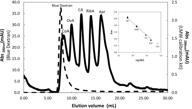
calibration kit void volumn (Vo) determination (Solid Line). Profile shows mixtureA and MixtureB, two different injections overlapped. See LMW Gel Filtration Calibration Kit protocol for details [151]. Insert - Calibration curve for the molecular weight determination using LMW Gel Filtration Calibration Kit. Kav = - 0.3771 Log (Mr) +1.9482. CoA was dispised due to Superdex 75 10/300 high molecular weight limit (75000 Da). Double Apr and RibA points corresponds to the same proteins in MixtureA and MixtureB for calibration of Superdex 75 10/300 GL, see LMW Gel Filtration Calibration Kit protocol for details [151]. The profiles correspond to independent injections.

Figure 16– Alignment of regulators protein sequences of CopR with known copper resistance regulators. Alignment was performed using Clustal X (version 2.0) [118].Legend: Green –

Dimerization interface; Dark green - Intermolecular recognition site; Yellow – Phosphorylation site; Turquoise – REC site; Gray – DNA binding site. Asterisk – Identical residues in all the alignment; Colon

– Conserved substitutions; Dot – Semi-conserved substitutions. For the accession numbers see Appendix B – Table 2 App.B.1(A).

Figure 17 – Alignment of the protein sequences obtained by the BLAST query of CopS and known copper resistance sensors. Alignment was performed using Clustal X (version 2.0) [118]. Legend: Green – ATP binding site; Dark green – G-X-G motif; Yellow – Mg2+ _{binding site; Turquoise –} Phosphorylation; Red – Dimer interface. Underlined – Transmembrane region. Asterisk – Identical residues in all the alignment; Colon – Conserved substitutions; Dot – Semi-conserved substitutions. For the accession numbers see Appendix B – Table 4 App. B.2 (B).

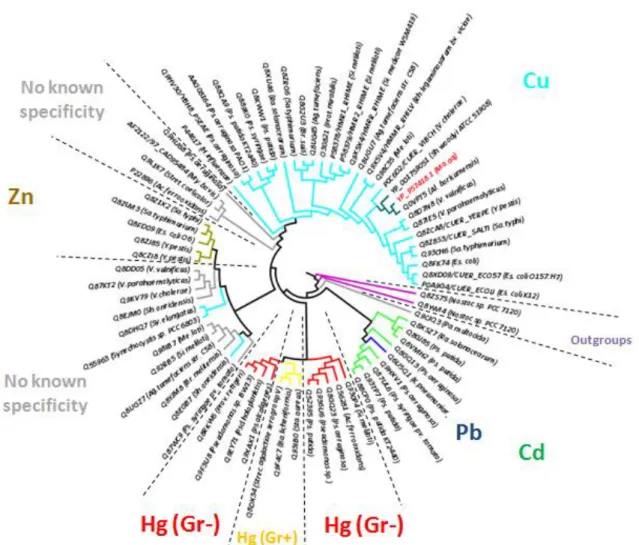
Figure 18 – Neighbor-joining algorithm regulators cladogram tree (proteins accessions numbers –

Appendix C – Table 7 App.C.1). Polar representation. Legend: Light blue - Cu ion region; Green - Cd; Dark blue - Pb; Yellow - Hg Gr+; Red - Hg Gr-; Gray - No known specificity; Teal - Ma.aq (studied sequences). Bootstrap values above 80% (data not shown for figure clarity). Clade distances relates to evolutionary distances. Identical to the other algorithms used, see Material and Methods, Chapter 2 –1.2 (data not shown).

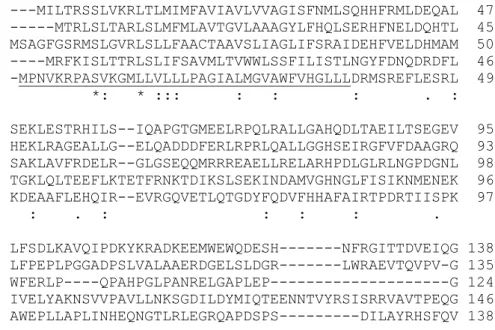
Figure 19 – Alignment of CopX with other blue type 1 copper protein (1) (proteins accessions numbers Appendix B –Table 6 App.B.3) and known copper resistant function protein (2), CopC. Legend: Gray residues correspond to type 1 blue copper protein motif. Asterisk – Identical residues in all the alignment; Colon – Conserved substitutions; Dot – Semi-conserved substitutions.

Figure 20 – Neighbor-joining algorithm CopX phylogenic inference (proteins accessions numbers Appendix C – Table 7 App.C.3). Legend: Blue - Known copper associated resistance proteins. Yellow - CopX (and homologous ORF and proteins). Black - Copper proteins. Clade distances do not relate to evolutionary distances. Homologs to the other algorithms used, see Material and Methods, Chapter 2 - 2.1 (data not shown).

Figure 21 – A) Ma.aqcontrol growth in ASW agar after 48 h incubation. B) Ma.aq growth in ASW

agar with 100 μM CdCl2 after 48 h incubation.

Figure 22 – Ma.aq growth curve in the presence of different cadmium ion concentration. The growths were followed for nearly 48 h. Legend:  0 CdCl2 (ASW control growth);  75 µM CdCl2;  100 µM CdCl2 and  250 µM CdCl2.

44

47 and 48

48 and 49

51

52

53

55

Figure 23 – A) Ma.aq control growth in ASW media agar plate, after 72 h incubation. B) Ma.aq

growth in ASW agar plate, in the presence of 0.5 mM CoCl2, after 72 h incubation. C)Ma.aq growth in ASW agar plate, in the presence of 4.0 mM CoCl2, after 96 h incubation. Arrows highlight isolated colonies for comparison.

Figure 24 – Ma.aq growth curve in the presence of different cobalt concentrations. The growths were followed for nearly 48 h. Legend:  0.75 nM CoCl2 (ASW control growth);  100 µM CoCl2; ▲750 µM CoCl2;  1.0 mM CoCl2.

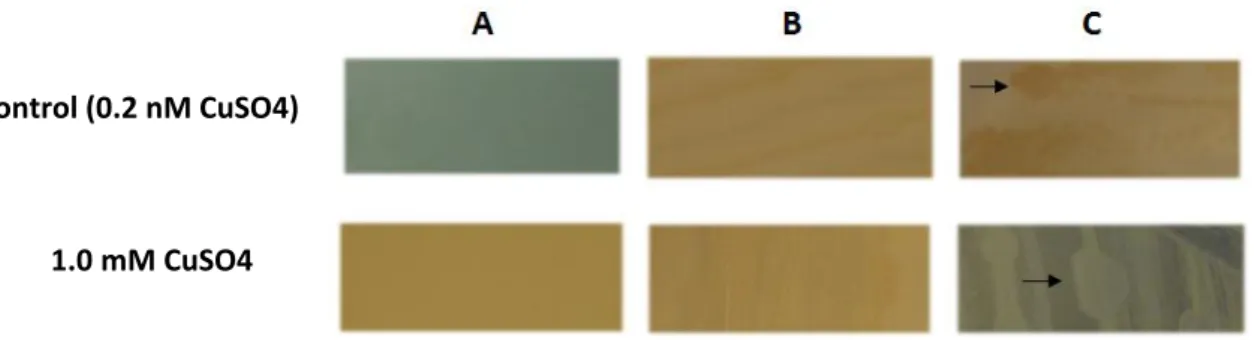
Figure 25 – ASW agar control plates and copper plates with a CuSO4 concentration of 1.0mM. (A) Control plate after 24h incubation. Plate containing 1 mM CuSO4 before inoculation (B), after inoculation and incubation for 24 h (C), and 120 h (control with dark background for picture clarity). Arrows highlight colonies differences.

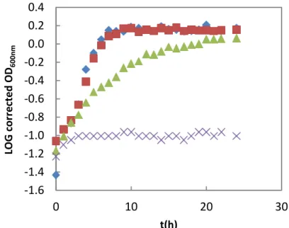
Figure 26 - Ma.aq growth curve of copper ion stress followed during 24h. Legend:  0.2 nM CuSO4 (ASW control growth);  100 µM CuSO4▲1.0 mM CuSO4 1.6 mM CuSO4.

Figure 27 – SDS-PAGE analysis of the cellular fractions of Ma.aq 617 grown under cobalt ion stress. Legend: 0 – control, 0.75 nM CoCl2; 1.0 – 1.0 mM CoCl2; MW – Low molecular weight marker. The samples were normalized by total protein content (10 µg). Arrow highlights possible differential proteins. 12.5 % polyacrylamide gel stained with Coomassie blue.

Figure 28 – UV-visible spectra of the periplasmatic fraction of the control growth, 0.75 nM CoCl2 (green line), and of the growth in the presence of 1.0 mM CoCl2 (blue line).

Figure 29 – 2D electrophoresis of the periplasmatic proteome of Ma.aq in 3-10 NL pH 13 cm Immobiline DryStrip. A) Control growth with 0.2 nM CuSO4 (30 µg protein applied); B) Copper stress growth with 1.0 mM CuSO4 (30 µg protein applied). 12.5% Acrylamide gel stained by Silver staining.Legend: White squares highlights region with visible differences

Figure 30 – 2D periplasmatic proteome electrophoresis of Ma.aq in 4-7 pH 13 cm Immobiline DryStrip. A) Control growth with 0.2 nM CuSO4 (30µg applied); B) Copper stress 1.0mM CuSO4 (30µg applied). 12.5% Polyacrylamide gel. Visualization method – Silver staining. Legend: Black and Blue circles indicate major highlights comparison.

Figure 31 – 3D view analysis of the low molecular weight area of the 2D gels presented in Figure 29. Images were obtained using GE 2D ImageMaster (Gray images) 7.0 and Ludesi REDFIN3 (Blue images). A) 0.2 nM CuSO4 periplasmic proteome. B) 1.0 mM CuSO4. Legend: Blue arrows correspond to protein spots only present in copper stress periplasmic proteome. Green arrows correspond to protein spots only present in control periplasm. Red plus and Black arrow indicate protein spot. Black circles – expected CopX area.

Figure 32 - 2D gel electrophoresis of the periplasmatic proteome of Ma.aq grown under copper stress (in the presence of 1 mM CuSO4; 60 µg of protein were applied to a 4-7 pH 13 cm Immobiline DryStrip. 12.5 % polyacrylamide gel. Legend: Dashed lines correspond to molecular weight migration experiments. Red circles indicate the protein spots analyzed. † Indicates protein spots analyzed from another gel (periplasmic fraction of a control growth, 0.2 nM CuSO4 but with 6 times more carbon source) and spot matching was performed using GE ImageMaster and Jvirgel 2.0 approach (Material and Methods, Chapter 2 –5.3). Visualization method – Coomassie blue.

light.

Figure 34 – A) Double digestion test of pET21c over time, with NotI and NdeI. Legend: 1kb – DNA ladder; 1 – Incubation time 1h; 2 – Incubation time 2h; 3 – Incubation time 3h; 4 – Incubation time 4h; Ctrl – Control undigested pET-21c(+). B) Purified double digested PCR product, copX, with NotI and NdeI. Legend: Incubation time 4h. 100bp – DNA ladder; 5 – copX double digested. C) Double digestion of pET-21c(+) with NotI and NdeI. Legend: Incubation time 4h. 1kb – DNA ladder; 6 – pET-21c(+) double digested; Ctrl – Control undigested pET-21c(+). All gel electrophoresis were run in 0.8 % agarose gel, stained with SybrSafe and visualized under blue light.

Figure 35 – Cloning vector pET-CopX (5975bp). Legend: DNA insert in orange, CopX (534bp). Cloning at the multiple cloning site, between NotI (located at 166 bp in pET21-c(+)) and NdeI (located at 238 bp in pET21-c(+)). Image was created using pDRAW32 (version 1.1.106) [165].

Figure 36 - pET-CopX clones screening. Syber safe under blue light visualization. Legend: 1 to 10 –

Colony number. 1kb - DNA ladder. 1% Agarose (image correspond to two different gels with colonies of the same plate).

Figure 37 – Positive clones screening. Syber safe under blue light visualization. Legend: 1 to 10 –

Colony number. 100bp and 1kb - DNA ladders. 1% Agarose (image correspond to two different gels with colonies of the same plate).

Figure 38 – Alignment of the nucleotide sequences obtained by the DNA sequencing (sequencing was performed by StabVida (www.stabvida.net)) from the 3 sent clones (1, 2 and 3) from the positive transformation, agains the reference gene, CopX (X) retrived from the Ma.aq VT8 chromosomal genome. Alignment was performed using Clustal X (version 2.0) [116]. Legend: Asterisk – Identical residues in all the alignment; Dot – Semi-conserved substitutions.

Figure 39 – Alignment of the amino acid sequences obtained by the DNA translation sequencing (sequencing was performed by StabVida (www.stabvida.net) and translation was performed by Expasy translate tool [164]) from the 3 sent clones (1, 2 and 3) from the positive transformation, agains the reference gene, CopX (X) retrived from the Ma.aq VT8 chromosomal genome. Alignment was performed using Clustal X (version 2.0) [116]. Legend: Asterisk – Identical residues in all the alignment.

Figure 40 – SDS-PAGE analysis of the expression profile of CopX in two growth media (LB and M9). Legend: MW – Molecular weight marker; 1 – Inoculum; 2 – LB before induction; 3 – M9 before induction; 4 – M9 2h IPTG induction; 5 – M9 4h IPTG induction; 6 – M9 7h IPTG induction; 7 - LB 2h IPTG induction; 8 - LB 4h IPTG induction; 9 - LB 7h IPTG induction; 10 – LB overnight IPTG induction. 12.5 % Polyacrylamide gel, stained with Coomassie blue.

Figure 41 - SDS-PAGE analysis of the periplasmic, cytoplasmic and membrane/insoluble fractions prepared from growths in rich and minimum media. Legend: MW – Molecular weight marker; 1 – Cytoplasmatic fraction; 2 – Periplasmatic fraction; 3 – Insoluble fraction. 12.5 % Polyacrylamide gel, stained with Coomassie blue

78

78

79

79

80 and 81

81

82

Figure 42 –UV-visible spectra of the periplasmatic fraction obtained from a growth in LB medium with 0.5 mM CuSO4 added in the inoculums moment, untreated fraction and oxidized with potassium ferricyanide.

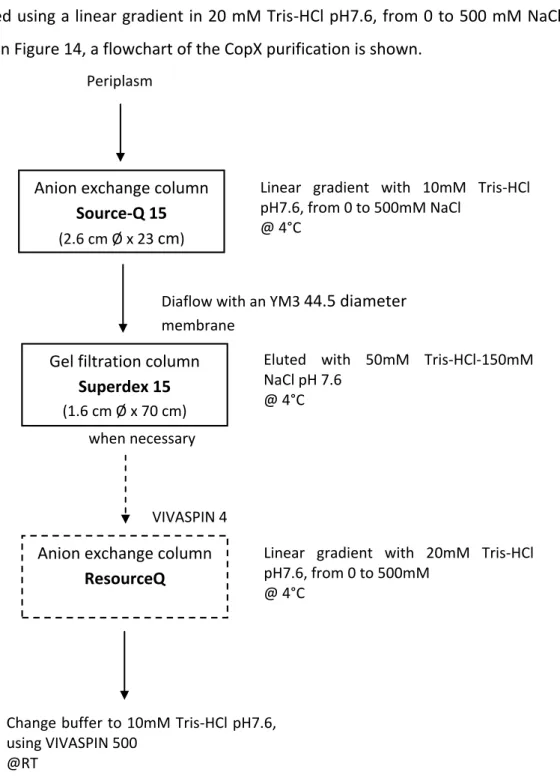
Figure 43 –– Elution profile of the first step of CopX purification, Source-Q 15. Legend: Black line - Protein content followed at 280nm. Gray line - Linear gradient in 10 mM Tris-HCl, pH7.6, from 0 to 500 mM NaCl. CopX eluted at 285 mM NaCl (highlighted with an arrow).

Figure 44 – Elution profile of the second chromatographic step of CopX purification, Superdex 75, eluted with 50 mM Tris-HCl, pH7.6, 150 mM NaCl. Protein content followed at 280nm. CopX peak is highlighted with an arrow.

Figure 45– Elution profile of the third step (optional) of CopX purification, ResourceQ 1 mL. CopX peak is highlighted with an arrow. Legend: (Gray line) linear gradient in 20 mM Tris-HCl, pH7.6, from 0 to 500 mM. (Black line) Protein content followed at 280 nm. CopX eluted at 285 mM NaCl.

Figure 46 – SDS-PAGE analysis of the different purification steps. Legend: MW – Molecular weight marker. PF – Periplasmatic fraction contained after expression of pETCopX in Es.coli BL21(DE3). S15 –

First chromatographic step, Source -15 column; S75 – Second chromatographic step, Superdex 75 column; RQ – Third chromatographic step, resource-Q column. 12.5% Polyacrylamide gel, stained with Coomassie blue.

Figure 47 – N-terminal sequence of the purified CopX. Legend: Underlined residues correspond to uncertained residues and X - amino-acids correspond to failed sequenced residue.

Figure 48 – CopX residue sequence. Legend: Gray highlights predicted signal peptide identified using SignalP 3.0 server [163]. Green highlights the N-terminal sequence i), in red bold correspondent residues; Brown bold highlights N-terminal sequence ii).

Figure 49 – UV-visible spectra of 27.3 M heterologously expressed CopX, in 10 mM Tris-HCl, pH 7.6. Legend: (Green line) Untreated CopX; (Blue line) Reduced CopX with sodium ascorbate; and (Red line) Fully oxidized with potassium ferricyanide.

Figure 50 – EPR spectra of 0.83 mM heterologous expressed untreated CopX in 10 mM Tris-HCl pH 7.6. Legend: Exp – Experimental result obtained using WinEPR (version 2.11) [169]; Sim – Simulated EPR spectrum obtained using and SimFonia (version 1.25) [170]. Experimental conditions: temperature 70K, 1 scan, microwave frequency 9.65 GHz, gain 105_{, attenuation 40 dB and} modulation amplitude 30 mT.

Figure 51 – Electro Spray ionization mass spectra of hetereologous expressed CopX in 50% ACN, 50% Water and 0.1% HCOOH. A) Mass-to-charge spectrum, the code at the top of each peak contains the number of positive charges for that m/z peak B) Deconvoluted spectrum. (The mass spectra was performed by Dr. Bart Devreese, in Belgium).

Figure 52- (Blue line) Elution profile ofheterologous expressed CopX in a Superdex 75 10/300 GL. Protein was eluted with 50mM Tris-HCl-150mM NaCl pH 7.6 at 4°C. (Black line) Elution profile of using LMW Gel Filtration Calibration Kit from a Superdex 75 10/300 GL Column eluted with 50mM Tris-HCl-150mM NaCl pH 7.6 at 4°C. Legend: Apr – Aprotinin, RibA – RibonucleaseA, CA – Carbonic Anhydrase, OvA – Ovalbumin, CoA – Conalbumin. Insert - Calibration curve for the molecular weight determination using LMW Gel Filtration Calibration Kit in Superdex 7510/300 GL. Trendline equation obtained Kav = - 0.3591 Log (Mr) +1.8352. CoA was dispised due to Superdex 75 10/300 high

Figure 53 – Ionic strength dependence of the apparent molecular weight ofCopX determined using Superdex 75 10/300 GL.

Figure 54 – 15_{N HSQC spectrum of 0.1 mM CopX in 10 mM NaPi, pH 6.0, 298 K. The spectrum was} acquired on a Bruker AvanceIII 600 NMR spectrometer equipped with a cryoprobe.

APPENDIX FIGURE INDEX

Figure 1 App.A. – Gene Ortholog Neighborhoods analysis of the putative copper operon, copSRXAB, from the Ma.aq chromosome using the copX (>) as the neighborhood reference (between dashed lines). Query was performed in Eubacteria (against genomes present at the DOE Joint Genome Institute databank). First, high similar, 7 obtained results are shown with the correspondent accession numbers. Legend: Same color genes belong from the same ortholog group, except light yellow that correspond to no ortholog assignment. White color corresponds to pseudo gene. Image obtained from the graphic interface Gene Ortholog Neighborhoods using the Integrated Microbial Genome system [116].

Figure 2 App.B.1(B) - Alignment of the nucleotide sequences obtained by the BLAST query of copR

and known copper resistance regulators. Alignment was performed using Clustal X (version 2.0) [118]. Legend: Asterisk – Identical nucleotides in all the alignment. For the accession numbers see Table App.3.

Figure 3 App.B.1(C) - Alignment of the peptides sequences obtained by the NCBI query of cueR (NP_752588.1) in Es.coli and Ma.aq CopR. Alignment was performed using Clustal X (version 2.0) [118]. Legend: Asterisk – Identical residues in all the alignment; Colon – Conserved substitutions; Dot

– Semi-conserved substitutions.

Figure 4 App.B.2(B) – Alignment of the nucleotide sequences obtained by the BLAST query of copS

and known copper resistance sensors. Alignment was performed using Clustal X (version 2.0) [118]. Legend: Asterisk – Identical nucleotides in all the alignment. For the accession numbers see App. Table 5.

Figure 5 App.B.2(C) - Alignment of the peptides sequences obtained by the NCBI query of Es.coli

CueS (NP_752587.1) and Ma.aq CopR. Alignment was performed using Clustal X (version 2.0) [118]. Legend: Asterisk – Identical residues in all the alignment; Colon – Conserved substitutions; Dot –

Semi-conserved substitutions.

Figure 6 App.C.2 – The tree of regulators from the E.A. Permina et al. 2005 study (Figure I). Different specificity is shown by the color code. Legend: Red and magenta are for negative and Gram-positive members of MerR subfamily, respectively. Light blue is for members of CueR and HmrR subfamily, green and deep blue are for members of CadR and PbrR subfamilies and orange is for members of ZntR subfamily. The identificators are given according to SWISSPROT Database. Black denotes regulators, whose specificity could not be specified. Figure from [120].

96

97

117

119 to 121

121

122 to 126

126 and 127

Figure 7 App.D.1 – CopX sequence was retrived from the Ma.aq VT8 chromosomal genome, locus coordinates 152394-152927. The sequence has 534 bp. Green highlight correspond to the START codon and red highlight correspond to the STOP codon.

Figure 8 App.D.2 – Graphical backbone representation of the expression plasmid, pET – 21c (+) (5441bp) used to clone copX. Image was retrived from EMB Biosciences – Novagen pET system manual [144].

Figure 9 App. D.3 – Restriction map of CopX, obtained using NEBcutter (version 2.0) [178].

Figure 10 App. E.1 – Selected OD values at 600nm of M.aq growth curve of cadmium ion stress followed during two days (nearly 48h). 0 h (inoculum moment), 24 h and 48 h of incubation.

Figure 11 App. E.2 – Temperature effect in plastes used in the solid assays. Control plates – 0.2 nM CuSO4 and stress plates 1.0 mM CuSO4. A) 24h incubation; B) 72 h incubation, C) 120 h incubation at 30 °C.

Figure 12 App. E.3– Selected low and high copper ion concentrations OD values at 600nm ofMa.aq

growth curve for copper ion stress. The growth was followed during two days (nearly 48h). 0 h (inoculums moment), 24 h and 48 h incubation at 30 °C.

Figure 13 App. F.1– UV–visible spectra of the Ma.aq citoplasmatic fraction of the control growth, 0.75 nM CoCl2 (green line), and of the growth in the presence of 1.0 mM CoCl2 (blue line).

Figure 14 App.F.2– UV–visible spectra of the Ma.aq membrane fraction of the control growth, 0.75 nM CoCl2 (solid green line), diluted 0.75 nM CoCl2 (dashed green line) and of the growth in the presence of 1.0 mM CoCl2 (solid blue line), diluted 1.0 mM CoCl2 (dashed blue line).

Figure 15 App G.1– 3D view and gel range variation analysis of the12.5% Polyacrylamide gel of 4-7 pH 13 cm Immobiline DryStrip run, highlighting the low molecular weight area, see Figure 30. A) Reference gel/control growth; B) Copper stress gel/growth in the presence of 1.0 mM CuSO4. Analysis was performed using Ludesi REDFIN3 [138].

Figure 16 App G.2 – 2D periplasmatic proteome electrophoresis of Ma.aq in 4-7 pH 13 cm Immobiline DryStrip. A) Control growth with 0.2 nM CuSO4 (30µg protein applied); B) Copper stress by 1.0 mM CuSO4 (30µg protein applied). 10% Polyacrylamide gel. Visualization method – Silver staining.

131

131

132 133

133

134

135

134

136

Table 1 – Composition of ASW medium. This solution is adjusted to pH 7.5 with HCl. The yeast extract was only added after the pH adjustment. Solution was sterilized by autoclaving. To prepare solid medium add 8 g/L of agar to the medium before autoclaving.

Table 2 – Compositon of Starkey, phosphate and iron solutions. The phosphate solution was sterilized by autoclave process and the Starkey and iron solutions were sterilized by filtration using

0.2 μM diameter filters (Sarstedt).

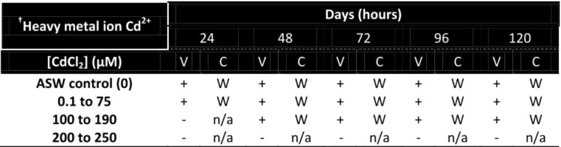
Table 3 – Results obtained in the determination of the MIC value for cadmium ions using solid media. Growth was followed during 5 days to register qualitative changes in the colony and media. Legend: V – Visible Growth; - No growth; + Growth; C – Colonies Color; W- White; n/a - Not applicable. Control ASW plates correspond to a non-stress growth of Ma.aq.

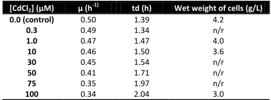
Table 4 – Specific Ma.aq 617 growth rate (µ) and generation time (td) of Ma.aq growths in the presence of difference CdCl2 concentrations. Values were determined from an exponential phase (1st to the 5th _{hour) semilog plot using logarithms to the base 10. Legend: n/r – not-recovered.}

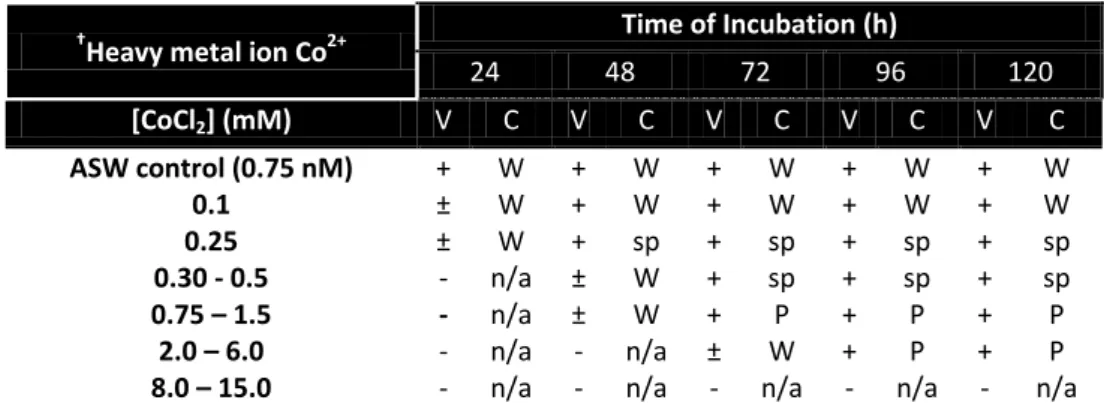
Table 5 – Results obtained in the determination of the MIC value for cobalt ions using solid media.

Ma.aq growth was followed during 5 days to register qualitative changes of colony and media. Legend: V – Visible Growth; - No growth; + Growth; C – Colonies Color; sp – Slightly pink; P – Pink; n/a - Not applicable. Control ASW plates correspond to a non-stress growth of Ma.aq.

Table 6 – Specific Ma.aq 617 growth rate (µ) and generation time (td) of cobalt ion stress concentration range tested by liquid media in Ma.aq. Values were determined by an exponential phase (1st to the 6th hour) semilog plot using logarithms of base 10.

Table 7 – Results obtained for the determination the Ma.aq MIC value for copper ions using solid media. The plates were incubated during 5 days to register changes in media and colony color and aspect. Legend: V – Visible Growth; - No growth; ± Small colonies; + Growth; C – Colonies Color; W- White; b – Slightly brown; B – Brown; n/a – Not applicable. Control ASW plates present 0.2 nM CuSO4.

Table 8 – Specific Ma.aq 617 growth rate (µ) and generation time (td) of the growth under copper ion stress. Values were determined by an exponential phase (1st to the 6th hour) semilog plot using logarithms of base 10. Legend: n/r – non-recovered.

Table 9 – Total protein content of cellular fractions obtained of the growths in the presence of different cobalt chloride concentrations.

Table 10 – Purification Table with the amounts of CopX recovered at the different stages of purification, for both media per L of growth with the CuSO4 added in the inoculum moment. Legend: n/p – not performed.

Table 11 – Values of the extinction coefficient (mM-1 cm-1) at 580 nm for heterologous expressed CopX.

Table 12 – Values used to simulate theCopX EPR spectrum.

APPENDIX TABLE INDEX

Table 1 App.A – BLAST score of the target gene for the ortholog study, copX (>).The algorithm used wasblastn (somewhat similar sequences) [117]. For the corresponding accession numbers see Figure App.1.

Table 2 App.B.1(A) – Accession numbers of the National Center for Biotechnology Information (protein sequence database) from the BLAST protein query of CopR (†), first 4 most similar sequences of known copper resistance regulators. Algorithm used was blastp (protein-protein BLAST) [117]. Table 3 App.B.1(B) - Accession numbers of the National Center for Biotechnology Information (nucleotide sequence database) from the BLAST nucleotide query of copR (†), first 4 most similar sequences of known copper resistance regulators. Algorithm used was blastn (somewhat similar sequences) [117].

Table 4 App.B.2(A) – Accession numbers of the National Center for Biotechnology Information (protein sequence database) from the BLAST protein query of CopS (†), first 4 most similar sequences of known copper resistance sensors. Algorithm used was blastp (protein-protein BLAST) [117].

Table 5 App.B.2(B) - Accession numbers of the National Center for Biotechnology Information (nucleotide sequence database) from the BLAST nucleotide query of copS (†), first 4 most similar sequences of known copper resistance sensors. Algorithm used was discontiguos megablast (more dissimilar sequences) [117].

Table 6 App.B.3 - Accession numbers of the National Center for Biotechnology Information (protein sequence database) from the BLAST protein query of CopX (†), first 4 most similar sequences of copper binding proteins. Algorithm used was blastp (protein-protein BLAST) [117]. Last protein was added for comparison with alignment Ps.sy CopC.

Table 7 App.C.1 – Accession numbers of the National Center for Biotechnology Information (protein sequence database) for proteins used in the phylogenic inference of Ma.aq CopR (†). Protein regulators are Eubacteria related heavy metal resistance regulators [120, 121].

Table 8 App.C.3 – Accession numbers of the National Center for Biotechnology Information (protein sequence database) for proteins used in the phylogenic inference of Ma.aq CopX (†). Sequences of copper-biding proteins and small copper proteins associated with copper resistance were used [120]. Table 9 App. G.3 – Maldi-TOF-TOF-MS analysis of the protein spots removed from the 2D gel electrophoresis, Figure 32. Legend: _† - Protein spots were analyzed from a different gel (periplasmic fraction of a control growth, 0.2 nM CuSO4 but with 6 times more carbon source).

Table 10 App.H.1 – Apparent molecular weight values of heterologous expressed CopX determined by size-exclusion chromatography at different [NaCl] in 50 mM Tris-HCl, pH 7.6.

118

119

119

122

122

127

128

130

137

INTRODUCTION

1. General Introduction

It was previously thought that resistance to heavy metals appeared as a result of the

recent year’s pollution. However, nowadays it is believed that it has been present since the

beginning of life, in an already metal-polluted world [1]. This idea is in line with the antibiotic

resistance determinants that are preexistent to recent human antibiotic handling [2, 3].

Although this is a clear conclusion for the antibiotic resistance, it requires caution when

referring to heavy metal resistance since it lacks experimental validation [1].

The heavy metals are 53 out of the 90 naturally occurring elements. This designation

is determined by the density value above 5 g/cm3. Almost, for each and every inorganic

cation or anion that is found in natural environments, organisms have mechanisms to

regulate their metabolic movement [3]. This specific complex homeostasis mechanisms

control their acquisition from the environment. Inside the cell, they control the

sequestration of the metal ions (that cannot be free inside the cell), by controlling the

expression of metal chaperones or other specific proteins that either store or expell the

excess of metal ions (heavy metals or metalloids) [4].

Since the origin of life, microorganisms have been exposed to heavy metal cations

and oxyanions, and the fact that these metal ions are able to form complex compounds

(redox-active or not) makes them essential trace elements, a feature that is related with the

unfilled d orbital of most heavy metals [3, 5].

Nevertheless, at higher concentrations most heavy metals are toxic. The toxicity is

related with the formation of unspecific complex compounds inside the cell that has toxic

effects. This can turn highly required trace elements into strong toxic complexes, which

makes them too dangerous for any physiological function. Therefore, the intracellular

concentration of heavy metals has to be tightly controlled [5].

Heavy metal resistance is just a specific component of the heavy metal homeostatic

system in each living cell. Throughout the years, several studies have discovered specific

genes and systems for transport of essential metals and for resistance to toxic heavy metal

The study of these systems is important because the insights into the interactions

between microorganisms and metals will be useful to understand the relation of toxic metals

with higher organisms, such as plants and mammals [7]. This knowledge has a vast

application, such as, in the study of copper transport diseases, like the Menkens and

Wilson’s diseases. These diseases are due to mutations in ATPases pumps, ATP7A in the case

of Menkes disease [8] and ATP7B in the case of Wilson disease [9], and these diseases are

related with copper starvation and copper excess, respectively. To strength this view, it was

found that those proteins are homologous to bacterial copper transport proteins. Therefore,

the understanding the bacterial versions of these ATPases pumps will contribute to a better

understanding of those diseases and possibly help finding a “cure” for them [10, 11].

Another example of an application is biotechnology. There are three main areas

where this could be achieved. First, adding metal resistance to a microorganism may

facilitate a biotechnological process, which may or may not be linked to heavy metals.

Second, heavy metal resistant bacteria may be used for bio-mining, either directly or by

recovering from effluents of industrial process. Third, use of heavy metal resistant bacteria

to bioremediation of metal-contaminated environments [5].

2. Biological important heavy metals

Although the definition of heavy metal is not consensus, there are 53 elements

considered as that, but not all of these are toxic. This is simply because some of the heavy

metals are not available in the ecosystems to the living organism, due to its low quantity in

the earth’s crust or its low solubility. To summarize these two factors, and distinguish the trace elements from the 53 existing heavy metals, sea water is used as an “average environment”. Depending on the concentration of these elements in sea water, they can be

grouped in four classes: frequent elements with concentration between 100 nM and 1 μM,

such as Fe, Zn and Mo; elements with concentrations between 10 nM and 100 nM, such as

Ni, Cu, As, V, Mn, Sn and U; rare elements, such as Co, Ce, Ag and Sb, and finally the ones

that exist at 1 nM level, such as Cd, Cr, W, Ga, Zr,Th, Hg and Pb. The remaining 31

The importance of the mentioned 22 heavy metals is directly related with the

solubility of their ions under physiological conditions, which eliminates Sn, Ce, Ga, Zr and Th

(insoluble), and to their toxicity which involves its affinity to sulfur and their interaction with

macrobioelements. From the 17 elements/heavy metals that are soluble, Fe, Mo and Mn are

important trace elements with low toxicity; Zn, Ni, Cu, V, Co, W and Cr are toxic elements

with high to moderate importance; and As, Ag, Sb, Cd, Hg, Pb and U, have limited beneficial

functions and are considered highly toxic [5, 12].

3. Heavy metal resistant bacteria

In bacteria, the heavy metal ions have to enter the cell in order to cause toxicity.

When inside the cell, the heavy metal cations, especially those with high atomic numbers,

tend to bind to -SH groups. The Minimal Inhibitory Concentration (MIC) or Maximum

Tolerant Concentration (MTC) of the metal ions is directly related with the complex dissociation constant of the respective sulphides. The binding of these metal ions to the

sulfide groups of proteins/enzyme can inactivate them and as a consequence inhibit

metabolic pathways [5].

In other cases, the cations of these heavy-metals can interact with the physiologic

ions inhibiting its function [5]. In gram-negative bacteria, cations can bind to glutathione

resulting in bisglutathionate complexes that react with oxygen species, and causes oxidative

stress [13]. Oxyanions can also interfere with related non-metal structures producing

radicals [5].

When the cell is in an environment with high concentrations of heavy metals, these

ions are transported to the cytoplasm, through unspecific transporters (constitutively

expressed) even when there are no metabolic needs. This “open gate” event is one of the

reasons why heavy metal ions are toxic. Indeed, it was observed that mutations in genes

coding for these transporters decreases the unspecific transport, and the organisms become

metal-tolerant [14].

However, many organisms have molecular systems for heavy metal resistance. One is

the ion efflux “pumping”, the most well-known bacterial heavy metal resistance system,

which can decrease the accumulation of heavy metal ions inside the cell. Another is the

into complex compounds rendering them insoluble and less toxic. Thirdly, the organism can

have molecular mechanisms for enzymatic detoxification (oxidation, reduction, methylation,

and demethylation) modifying the heavy metal ion to a less toxic or less available form.

Many heavy metal homeostasis and resistance system can involve two or three of these

mechanisms [2, 5, 15].

Another mechanisms that can be considered important for resistance is the

bio-accumulation (intracellular or at the cell surface) or bio-sequestration (conversion of the

toxic ion through biological processes – “indirect” resistance system) [2].

Addressing the heavy metal metabolism, detoxification by reduction can only occur if

the redox potential of the heavy metal is between the hydrogen/proton couple (- 421 mV)

and the oxygen/hydrogen couple (+ 808 mV) (at 30°C and pH 7.0, which is the physiological

redox range for most aerobic cells [12]. After reduction, the metal ion has to diffuse out of

the cell to avoid re-oxidation. Therefore, the organism must present an efflux system to

export the reduced metal ion. For a fast-growing organism, the cost of complexation for

efflux is very high. Thus, complexation occurs mainly at low metal concentrations. Therefore,

detoxification through efflux systems, alone or in combination, is the only possible option for

a fast-growing organism in an environment contaminated with high concentrations of heavy

metals. Thus, heavy metal metabolism can be described as transport metabolism [16].

3.1 Heavy metal transporters

The ion uptake by the cell is directly dependent of its structure. Looking at the ions

structure, all mono- or divalent cations are small and structurally very similar, when

compared with oxyanions that differ widely in structure and are bigger. Thus, uptake

systems have to bind the metal ions tightly to differenciate them, which is possible at the

cost of energy [17].

The transport of toxic cations or oxyanions found in bacterial resistance systems are

mainly ATPase membrane pumps and chemiosmotic membrane pumps. These systems can

be divided into seven major types:

- Two types of ATPases:

located in the inner (cytoplasmic) membrane and they can transport ions to the cytoplasm

or can operate as expulsion systems, removing ions from the cytoplasmatic space.

Nevertheless, these ATPases need to be associated to outer membrane proteins to expel the

ions to the exterior. The members of the P-type ATPases present eight transmembrane

helices (TM), a large citoplasmatic region that binds to ATP (ATPBD, composed of N and P

domains) and also several cysteines residues that “trap” the ions that are being expelled

(actuator A domain) (Figure 1). Between the transmembrane helix six and seven there is a

proline residue preceded by a probable metal-binding residue, the CPX motif that is

essencial for its function. At the N-terminal, there is a soluble metal binding domain (MBDs)

(Figure 1) [7, 18, 19].

Figure 1– Overall architecture of Cu (I) P-type ATPases. The number of MBDs at the N-terminus ranges from one to six depending on the organism [19].

(2) ABC ATPases (ATP binding cassette without phosphorylated intermediates) consists of a cytoplasmatic membrane associated with an ATPase subunit, one or two

membrane embeded pump channels, an ion-binding protein, and an outer membrane porin

protein. In bacteria, the ABC ATPases are organized in four domains, requiring additionally a

binding protein (Figure 2). The pumps of this family do not function as metal ions efflux

systemm, only uptake [20, 21].

- Five efflux pump classes that are chemiosmotic ion/proton exchangers:

(3) the single membrane polypeptides of the Major Facilitator Superfamily (MFS), generally a single polypeptide that transverses the membrane 12 or 14 times primarily in an

alpha helical structure (Figure 3) [22, 23].

Figure 3 – Schematic model of the membrane topology of MFS proton-driven pumps in Gram-negative bacteria. Adapted from [23].

(4) the Cation Diffusion Facilitator (CDF) family [24] are medium size polypeptides (less than 400 residues), with six transmembrane segments, that function as homodimer in

the inner membrane and are H+ antiporter (for metal efflux) or H+ symporter (for metal

uptake). In this chemiosmotic ion transport process there is the participation of histidine

(HRR – histidine-rich region), aspartate and glutamate residues (Figure 4) [7, 25].

Figure 4 – Model of an CDF family protein [25].

(5) The Resistance-Nodulation-cell Division (RND) superfamily are transporters that have different roles in bacteria, namely resistance, nodulation and cell division. The inner

membrane segment is composed of around 1000 residues, that expelles the ions. The

auxiliary segments are a small protein from the outer membrane, and a protein that

connects the outer and inner membrane segments, forming a complex that spans over the

Figure 5 - Schematic representation of aRND efflux system in gram-negative bacteria. Adapted from [28].

- The last two chemiosmotic pumps have narrower substrate range:

(6) the Chromate efflux system (CHR) [29], and

(7) the Arsenite and Antimonite efflux systems that can function alone or with energy from ATP, being named as A-type ATPases [30].

There are two other transport system that differ from the ones presented above, the

mercury uptake system [31] and the arsenic efflux system [32] which constitute their own group [15, 33].

3.2 Heavy metal repressors and activators

Bacterial chromosomes have genes for transport and/or for confering resistance to

inorganic nutrient cations and oxyanions (such as NH4+, K+, Mg2+, Co2+, Fe3+, Cu2+, Mn2+, Zn2+),

to other trace cations, to PO3-4 and SO2-4, and to other less abundant oxyanions [3]. There

are also bacterial vectors that present genes for resistance to metals ions, such as Ag+, AsO2-,

AsO43-, Cd2+, Co2+, CrO42-, Cu2+, Hg2+, Ni2+, Sb3+, TeO32-, Tl+ and Zn2+. Plasmid resistance to

B4O72-, Pb2+ and organo-tin compounds has also been reported [2] [3]. Together, this

genetically-defined resistance accounts for a few hundred genes [3].

All bacterial heavy metal resistance systems are constituted by regulons, sometimes

as operons (units of mRNA transcription), or clusters of contiguous genes (from two to more

than ten) regulated by a protein that binds to the upstream operator DNA regions. Metal

of transport and storage proteins. In general, there are four classes of metal-responding

transcriptional regulators:

(1) the Mer family of homo-dimeric activator proteins that bind to usually long 10-35 RNA polymerase-binding operator regions, with 19 or 20 nucleotide spacing [34];

(2) the ArsR/CadC/SmtB family, which act negatively, binding to the 17-spaced –

10-35 operator region preventing the binding of the RNA polymerase. When the protein binds

to the co-repressor ion, the repressor is released from the DNA allowing transcription of the

genes controlling the resistance to the metal ions [35];

(3) the two-component systems, in which the transmembrane histidine kinase membrane sensor (S) autophosphorylates at a conserved His residues, in response to an

extracellular stimulus. The phosphate is then transferred to a conserved aspartate on the

second responder (R) regulatory protein, which is then either activated or inactivated for

DNA-binding transcriptional control [36];

(4) the YXH complexes, in which the H proteins are sigma factor subunits of RNA polymerase and respond to environmental cation addition, and the Y and X proteins bind to

anti-sigma factors. Multiple promoter sites are found, one for the regulatory genes and

another for genes determining the efflux pump [37].

In addition to the first level of regulatory proteins there is a second level. These

proteins are directly involved in gene regulation and are at the same time chaperones:

intracellular carrier proteins with the role of picking up the toxic ions, reducing their free

cellular levels, and specifically transfering the inorganic ion to the transcriptional regulator

or to other specific protein that binds metals ions as a cofactor [38].

4. Cadmium and Cobalt bacterial mechanisms

Cadmium has almost no known biological function, and can lead to cell damage and death even at low concentrations [39].

On the other hand, cobalt is an essential micronutrient for many bacteria, as a

cofactor in different enzymes that catalyze a diverse array of reactions, such as production

of adenosylcobalamin (one of the two natural cofactor forms of vitamin B12). Cobalt is