Rational Choice with Categories

Rational Choice with Categories

∗

Bruno A. Furtado

Leandro Nascimento

Gil Riella

February, 2017

Abstract

We propose a model of rational choice in the presence of categories. Given a subjec-tive categorization of the space of alternasubjec-tives, the choosable alternasubjec-tives from a given choice problem are the ones which are optimal inside at least one category. Represen-tation theorems are given in which the decision maker always satisfies a weaker form of the Weak Axiom of Revealed Preference and different postulates are imposed on a gen-eral notion of revealed preference relation. They identify a class of choice functions that is nested between choice functions represented by multiple rationales and the standard model of rational choice. In particular, our weaker model of categorization generalizes the maximization of incomplete preferences, and is a special case of what is called a pseudo-rational representation. When we have pairwise disjoint categories, the unique representation becomes a special case of the maximization of an incomplete preference relation, while the model reduces to standard rational choice when there is only one category. Finally, we show that the main insights we learn in the deterministic choice setup can sometimes be exported to other setups. As examples, we show how the ideas developed here can be used to derive categorization models in the setups of random choice and preferences over menus.

JEL classification: D01, D60

Keywords: Categorization, weak categorization, rational choice, pseudo-rational choice, incomplete preferences.

∗_{We thank Pietro Ortoleva for very helpful comments. Riella gratefully acknowledges the financial support} of CNPq of Brazil, grant no. 304560/2015-4.

†_{Ministério da Fazenda do Brasil. E-mail: bruno.furtado@fazenda.gov.br.}

‡_{Departamento de Economia, Universidade de Brasília. E-mail: lgnascimento@unb.br.}

1

Introduction

Choice behavior is frequently based on heuristics. Especially in situations involving a wide range of choices, people rarely make a fully rational deliberation and employ instead heuris-tic procedures to first reduce the complexity of the problem they face and only then make a decision (Payne, 1976; Payne et al., 1988). In fact, in many problems of individual choice the decision maker (henceforth DM) is not able to express preferences over all pairs of alter-natives, and decides what category to spend her money on before screening the alternatives within the relevant category (Schwartz, 2000), or allocates her income into different cate-gories of bundles of goods and selects the best alternative from each one (Heath and Soll, 1996). Here the DM compartmentalizes her world into categories and need not necessarily behave as if there were a single category containing all conceivable and completely ranked alternatives as in the standard model of rational choice.

Examples of decision-making procedures which employ a categorization of the choice set are well documented and range from ordinary consumer purchase decisions (e.g., Gutman, 1982; Cohen and Basu, 1987) to portfolio allocation and long-term planning decisions made by investors (see Barberis and Shleifer, 2003). They are all based on the intuitive idea that, especially during the process of making decisions, people group their alternatives into differ-ent sets or classes of objects that are somehow related. Indeed, categorization is considered one of the most fundamental and pervasive cognitive procedures, functioning as an organiz-ing principle that helps us obtain the maximum information from the perceived world with the least cognitive effort (Rosch, 1978).

Even though categorization and concept formation have central roles in the study of cog-nition, and therefore of rationality, they are seldom explicitly taken into account in economic models. In fact, a recurring criticism of the standard theory of rational choice is that it fails to take into account the role of category formation to the human decision-making process, in spite of its importance in many applications. We therefore develop a model that departs from the traditional rational choice framework precisely in that it allows for categorization to play a key part in the choice process.

This paper examines the properties of a choice function where choices are represented by the union of the best alternatives available from each category according to a preference relation (a reflexive and transitive binary relation) that is complete inside each category. More formally, given a grand set of alternativesX, a family of choice problemsΩX ⊆2X\{∅},

and a choice function

we give in this paper an axiomatic characterization of a DM who divides the space of alter-natives into a collection of categories S, has a preference relation % on X that is complete inside each category S ∈ S, and makes her choices by selecting the most preferred elements from each category. In other words, if we denote the set of maximum elements in Y with respect to R by max(Y, R) := {x ∈Y : xRy for all y ∈ Y}, for any set Y ⊆ X and binary relationRonX, we characterize a choice function that can be represented by the expression

c(A) = [

S∈S

max(A∩S,%), for every A∈ΩX. (2)

We will refer to the representation in (2) as a weak categorization representation if the categories in S are allowed to intersect each other, and we will call it a categorization repre-sentation whenever S is a partition of X.

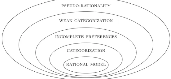
It turns out that the weak categorization and categorization models described above are nicely nested among some traditional models in the rational choice literature. For example, the weak categorization model is a special case of the very general pseudo-rational repre-sentation axiomatized by Aizerman and Malishevski (1981). Recall that the pseudo-rational representation is composed of a set of rationales and the choosable alternatives in each choice problem are the ones that maximize at least one of the rationales.

We also show that weak categorization is a more general model than the maximization of a possibly incomplete preference relation, while categorization is a special case of that type of representation. Finally, the rational choice model, that is, the model that maximizes a single complete preference relation, is simply a categorization model with only one category. Figure 1 summarizes all these connections.

pseudo-rationality

weak categorization

incomplete preferences

categorization

rational model

Looking closely at the connections between the categorization models and the other mod-els described above, we identify a general rationality postulate, which is a natural relaxation of the Weak Axiom of Revealed Preference (WARP) that is satisfied by all models discussed in this introduction. Moreover, at least in finite choice spaces, all the differences among the models above can be captured by variations on the properties satisfied by a general notion of revealed preference we discuss here.

Interestingly, we observe that the main insights we develop here in a deterministic choice setting can sometimes be applied even when the available data is in a different format than a deterministic choice function. Specifically, we show how the same principles used in a deterministic choice setting can be utilized to obtain versions of the weak categorization and categorization models when the data available is in the form of a random choice function or a preference relation over choice problems (preferences over menus). For example, in the random choice setup, if we start with a random choice function that has a random orderings (or random utility) representation, which is in some sense the natural translation of the pseudo-rational model to that setup, we arrive at the weak categorization model by imposing the acyclicity of a suitably defined notion of revealed preference, which is also the property that characterizes weak categorization representations in a deterministic choice setup. Similarly, the version of the categorization model in the setup of random choice is obtained through a natural translation of the postulate used in the deterministic choice setting to that setup. These very same steps also deliver versions of our categorization models in the preferences over menus setup. In the case of preferences over menus, the model we consider to be the natural translation of the pseudo-rational model is the subjective state space representation introduced by Kreps (1979).

that the random choice function has a random orderings representation. Finally, we relegate all proofs of the results presented in the main text to Appendix D.

2

Setup and Definitions

For an arbitrary set X, a binary relation % on X is simply a subset of X ×X. As usual, we write x%y to represent the fact that (x, y)∈ %. We say that % is reflexive ifx%x for every x∈ X, and say it is transitive if x %y and y %z imply x% z, for everyx, y, z ∈X. A reflexive and transitive binary relation is called a preorder or a preference relation. Given a subset Y of X, we say that % is complete on Y if, for every x, y ∈ Y, we have x % y or

y % x. The symmetric and asymmetric parts of % are denoted by ∼ and ≻, respectively. Formally, for eachx, y ∈X, x∼y if x%yand y %x, andx≻y if x%y, but it is not true that y % x. Finally, we say that % is antisymmetric if ∼ ⊆ {(x, x) : x ∈ X}. We call an antisymmetric preorder a partial order.

Now, letX be any set and letΩX be a collection of nonempty subsets ofX. We interpret

X as the grand set of alternatives andΩX as the collection of all conceivable choice problems

the DM may face. For notation, we denote byF(X)the set of all finite and nonempty subsets of X.

We will follow Eliaz and Ok (2006) and work with the following definition:

Definition 1. We say that(X,ΩX)is a choice space if

(i) {x} ∈ΩX for every x∈X;

(ii) A∪B ∈ΩX whenever A, B ∈ΩX.

In words, the definition above says that (X,ΩX)is a choice space whenever all singletons

belong to ΩX, and ΩX is closed under finite unions. Given a choice space (X,ΩX), we say

that a functionc: ΩX →2X\ {∅}is a choice function wheneverc(A)⊆Afor everyA∈ΩX.

We can now formally introduce the models of categorization that are the subject of this paper.

Definition 2. LetX be an arbitrary set and% a preorder on X. Aweak categorization of

the set X relative to % is a family S of nonempty subsets of X such that X = ∪S and % is complete on every S ∈ S. Any S ∈ S is referred to as a category. If in addition all sets

S ∈ S are pairwise disjoint, so that S is a partition of X, we say that S is a categorization

of X relative to %.

individual to have Chinese Food as a category, with Chinese Noodles as a separate category within the first, and another category, say Pasta, that also contains Chinese Noodles but is not a subset of Chinese Food. Such intersecting categories may arise if, for example, multiple criteria are used for the categorization procedure, and these criteria overlap. For instance, television sets can be categorized according to size, price range, brand and picture quality, and hotels by service, comfort and location.

Implicit in the definition above is the idea that categories are, at least in part, subjec-tive. Notice that the manner in which the DM categorizes alternatives is dependent on her (subjective) preferences. Thus, categories are not assumed to be observable, except perhaps indirectly from the DM’s choice behavior. An outside observer cannot assume, for instance, that Chinese Food and Mexican Food will be relevant categories to the DM in any particular application. This is in line with studies in cognitive psychology, which reveal disagreement among individuals about which categories certain objects belong to (e.g., Mervis and Rosch, 1981), and also suggest that the type of categorization process used by an individual – whether it is rule-based or similarity-based, for instance – impacts the resulting categories in a predictable way (Smith et al., 1998).

Definition 3. Given a choice space(X,ΩX)and a choice functioncon(X,ΩX), we say that

c admits a weak categorization representation if there exist a preorder % on X and a weak categorization S of X relative to % such that c can be expressed as in (2). If S is in fact a categorization ofX relative to%, then we say thatcadmits acategorization representation.

In a categorization or weak categorization representation, the choice function c selects the best elements from each category among the available alternatives. That is, the set

is indeed indifferent between them.

3

Representation Theorems

In this and the next section we will restrict our attention to finite choice spaces. That is, we will assume that X is a finite set andΩX := 2X\ {∅}. Letcbe a choice function on(X,ΩX).

As we have discussed in the Introduction, the analysis here will be based on a general notion of strict revealed preference. Formally, consider the following definition:

Definition 4. Define the binary relation⊲⊆X×X byx⊲y if, and only if, there exists a

choice problemA ∈ΩX such that y∈c(A) but y /∈c(A∪ {x}), for anyx and y in X.

In words, the relation ⊲ declares x to be preferred to the alternative y if there exists at least one situation where y stops being chosen because x is added to the set of available alternatives.

Throughout the paper our axioms will always imply that the binary relation ⊲ is asym-metric (that is, x⊲y implies that y⊲x is not true), so that we can indeed interpret it as a form of strict revealed preference. As we have discussed in the Introduction, all models studied in this paper satisfy a basic rationality property and differ from each other only with respect to the properties of the relation ⊲. Formally, consider the following weakening of the standard Weak Axiom of Revealed Preference (WARP):

Axiom 1 (Pseudo-WARP). For all A, B ∈ΩX: if x ∈c(B)∩A and c(B∪ {y})⊆B for

ally∈A, thenx∈c(A).

As we have said above, Pseudo-WARP is a basic rationality property satisfied by several models. In that postulate, x is one of the choices from the set B and x also belongs to

A. On top of that, none of the alternatives in A\B is good enough to become a choice when added toB. When this happens, Pseudo-WARP demands thatxbe also a choice from

A. In contrast to that, WARP says that x must belong to c(A) whenever c(A)∩B 6= ∅. Since WARP implies that y ∈ c(B ∪ {y}) for any alternative y ∈ c(A∪B), we must have

(A\B)∩c(A∪B) =∅whenever c(B∪ {y})⊆B for every y∈A. But then c(A∪B)⊆B

and, by WARP, this can happen only if x ∈ c(A∪B). Applying WARP again, we obtain that x∈c(A). This shows that WARP is indeed stronger than Pseudo-WARP.

Axiom 2 (Acyclicity). The binary relation ⊲ is acyclic. That is, for any finite collection

{x1, . . . , xn} ⊆X, ifx1⊲· · ·⊲xn, then it is not true that xn⊲x1.

Acyclicity can also be seen as some basic rationality postulate imposed on the indirectly revealed strict preference relation ⊲. We note that if a choice function c has a weak cate-gorization representation (%,S) and x⊲y for some pair of alternativesx, y ∈X, then it is clear that we must have x ≻ y. Therefore, the fact that the acyclicity of the relation ⊲ is a necessary condition for a choice function c to have a weak categorization representation is an immediate implication of the transitivity of the preorder % that is part of that type of model. At the same time, it is easy to verify that any choice function that has a weak categorization representation satisfies Pseudo-WARP. Our first main result shows that these two postulates exactly characterize the choice functions which admit a weak categorization representation.

Theorem 1. LetX be a finite set andc be a choice function on(X,2X_{\ {∅}). Thenchas a}

weak categorization representation if, and only if, it satisfies Pseudo-WARP and Acyclicity.1

Theorem 1 is an immediate corollary of Theorem 11 below, so we omit its proof. Still, it is important to mention that two aspects of our axioms are key to the sufficiency part of the proof of Theorem 1. First, they imply that if an alternative x is chosen from a choice problem A, then it is also chosen from all choice problems smaller than A in whichx is still available. We refer to this property as Chernoff’s axiom or Sen’s α postulate (see Section 4 below). Second, they imply the existence of an acyclic binary relation≻∗ _{onX such that, for}

any pair of choice problems Aand B inΩX withB ⊆A, ifx∈X is such thatx∈c(B), but

it is not true that x∈c(A), then there existsy∈A\B with y≻∗ _{xand y∈c(B∪ {y}). We}

can see this property as a partial form of binariness (representability by a binary relation), since, for every A∈ΩX and x∈A, x∈max(A,≻∗) :={y ∈A:for no z ∈A it is true that

z ≻∗ _{y} impliesx∈ c(A). Moreover, it turns out that these two properties characterize the}

choice functions that admit a weak categorization representation even in arbitrary choice spaces. We have a detailed discussion of this fact in Appendix A.

We now turn to the case of a DM who divides the set of alternatives into a family of pairwise disjoint categories. Here we are taking into consideration that in many particular applications the process of categorization gives rise to disjoint categories, and every element of the choice set must belong to one, and only one, category. For instance, if the only relevant categories for a DM are Food and Shelter, it is unlikely that any given element of

1_{Theorem 1 does not actually require the grand set of alternativesXto be finite. It is sufficient to assume} that every choice problem is a finite set, that is,ΩX =F(X). Therefore, the axioms also characterize a weak

the choice space will belong to both groups. More broadly, according to the more classical view of categorization held in psychology and philosophy, going back to Aristotle, categories are discrete entities whose elements obey necessary and sufficient conditions for membership, and should be clearly defined, mutually exclusive and collectively exhaustive. Categories are thus disjoint by definition.2

Again, the analysis will rely on the properties of the relation ⊲. In particular, we will have to restrict how ⊲interacts with the DM’s choices from two-element sets. We will need the following definition, from Ribeiro and Riella (2017):

Definition 5. Let (X,ΩX) be a choice space and c a choice function on ΩX. We say that

x, y ∈X are behaviorally indifferent if, for every A∈ΩX,

(i) x∈c(A∪ {x}) if, and only if,y ∈c(A∪ {y});

(ii) c(A∪ {x})\ {x, y}=c(A∪ {y})\ {x, y}.

As Ribeiro and Riella (2017) point out, two alternatives x and y are behaviorally indif-ferent if they are practically indistinguishable in terms of choices. It is as if one alternative is simply a duplicate of the other.

Given a set A, we write |A| to represent the cardinality of A. We can now state the following postulate:

Axiom 3 (Compatibility). For allx, y, z ∈X: if x⊲y, then|c({x, z})|=|c({y, z})| orz

is distinct fromx and y, but behaviorally indifferent to one of them.

Define a binary relation ⊲∗ ⊆X×X byx⊲∗yif, and only if, {x}=c({x, y}), for every pair of distinct alternativesx, y ∈X. There are two forces behind the compatibility axiom. First, in the presence of Pseudo-WARP, it implies that the revealed preference relation ⊲ is completely characterized by choices from two-element subsets of X. That is, ⊲ = ⊲∗. Now suppose that x⊲y and pick an alternative z distinct from x and y. The compatibility postulate then imposes that, unlessz is behaviorally indifferent toxory, we must have that

x and z are strictly ranked according to ⊲∗ _{if, and only if, y and z are also strictly ranked}

according to⊲∗_.

The next theorem shows that Pseudo-WARP and Compatibility are necessary and suffi-cient conditions for a choice function to have a categorization representation. It also char-acterizes the uniqueness properties of this type of representation.

Theorem 2. Let X be a finite set and cbe a choice function on (X,2X _{\ {∅}). Then c has}

a categorization representation if, and only if, it satisfies Pseudo-WARP and Compatibility. Moreover, two categorizations (S,%) and(S′_,%′_{)represent the same choice function if, and}

only if, {S ∈ S : max(S,%)6= S} = {S ∈ S′ _{: max(S,%}′_{) 6=S}, and %, %}′ _{coincide inside}

any of the categories in the collection {S ∈ S : max(S,%)6=S}.

Theorem 2 is an immediate corollary of Theorem 12 below, so we also omit its proof. We note, however, that Theorem 2 characterizes which choice functions admit a categorization representation and also shows that this type of representation has strong uniqueness prop-erties. Given a categorization (S,%), let’s agree to call a category S degenerate if x ∼ y

for every x, y ∈ S. In words, the uniqueness part of Theorem 2 says that all categorization representations of the same choice function have exactly the same non-degenerate categories and agree on how to compare any pair of alternatives that belong to the same category of that type. Therefore, two different categorization representations of the same choice function can disagree only on the collection of degenerate categories. Notice, however, that this disagree-ment is completely immaterial, since you can always redistribute the degenerate categories anyway you want without affecting choices.

As we have discussed in the Introduction, the categorization models discussed in this section connect several traditional models of the literature on rational choice. In the next section, we show how we can keep Pseudo-WARP and vary only the properties of the revealed preference relation⊲in order to characterize models that range from the very general pseudo-rational model of Aizerman and Malishevski (1981) up to the standard pseudo-rational choice model, where the DM maximizes a complete preorder.

4

Rational Choice and Categorization

Our models of choice with categories can be placed within the wider context of rational choice by recalling Figure 1. Moreover, Pseudo-WARP can be seen as a very basic ratio-nality postulate and, as we shall see soon, all the models in Figure 1 are characterized by different properties of the binary relation⊲. We begin by recalling the definition of a pseudo-rationalizable choice function, first axiomatized by Aizerman and Malishevski (1981).3

Definition 6. Given a choice space (X,ΩX) and a choice function c on (X,ΩX), we say

that c has a pseudo-rational representation if there exists a family P of complete preorders onX such that

c(A) = [ %∈P

max(A,%),

for every A∈ΩX.

Two classical axioms introduced by Chernoff (1954), Postulates 4 and 5∗_{, characterize}

the choice functions that have a pseudo-rational representation. They are subsumed by the following equivalent (in finite choice spaces) version of Pseudo-WARP.

Axiom 4 (Pseudo-WARP∗_{). For all A, B ∈ Ω}

X: if x ∈ c(B)∩A and c(A) ⊆ B, then

x∈c(A).

Pseudo-WARP∗ contains two general principles of rational choice. One is Chernoff’s axiom, which was discussed in the previous Section. The second principle asserts that when more options are added to the set of alternatives and none of the new options is chosen, the choices from the smaller set are also choices in the larger set of alternatives. This principle expresses a weaker form of binariness than is assumed in the traditional model of rational choice (namely, that every element that is chosen in pairwise comparisons with the alternatives in a given set it belongs to is also a choice from the set). It is sometimes referred to as Aizerman’s axiom.

Chernoff ’s Axiom For allA, B ∈ΩX with B ⊆A: c(A)∩B ⊆c(B).

Aizerman’s Axiom For all A, B ∈ΩX with B ⊆A: if c(A)⊆B then c(B)⊆c(A).

We have the following result:

Theorem 3. LetXbe a finite set. A choice functioncon(X,2X_{\{∅})has a pseudo-rational}

representation if, and only if, it satisfies any of the following conditions.4

(i) Chernoff and Aizerman’s axioms. (ii) Pseudo-WARP.

(iii) Pseudo-WARP∗_.

It should be remarked that Theorem 3 breaks down in arbitrary choice spaces. In fact, we are not aware of any axiomatization of pseudo-rational choice functions when the choice space is not finite. We note, however, that Pseudo-WARP is still a necessary condition for a pseudo-rational representation even in arbitrary choice spaces. As the next example shows, the same is not true for Pseudo-WARP∗ nor Aizerman’s axiom.

Example 1. Assume thatX :={x1, x2, . . .}is a countably infinite grand set of alternatives,

with xk+1 ≻1 xk for all k ≥ 1, x1 ≻2 xk for all k ≥ 2, and xk ∼2 xl for all k, l 6= 1. Then

c({x1, x2}) = {x1, x2} but c(X) = {x1} and thus c({x1, x2}) *c(X). Therefore, c does not

satisfy Pseudo-WARP∗ _{nor Aizerman’s axiom, while it has a pseudo-rational representation}

and, consequently, satisfies Pseudo-WARP

When we compare Theorem 3 with Theorem 1, we see that only the acyclicity of the binary relation ⊲ separates weak categorization from pseudo-rationality. The next exam-ple confirms that pseudo-rationality is indeed a strictly more general concept than weak categorization.

Example 2. Let X := {x, y, z, w} and consider a choice function c pseudo-rationalized by

the linear orders y ≻1 x ≻1 z ≻1 w and w ≻2 z ≻2 x ≻2 y. Since x ∈ c({x, y}) but

x /∈c({x, y, z}), we have z⊲x. On the other hand, sincez ∈c({z, w}), butz /∈c({x, z, w}), we also havex⊲z, thus violating Acyclicity. Therefore,cdoes not have a weak categorization

representation.

An important special case of a weak categorization representation is the maximization of a possibly incomplete preference relation. In finite choice spaces, this type of representation is characterized by Pseudo-WARP plus a version of Compatibility that links the baseline revealed (strict) relation ⊲ and the strict preferences revealed in binary choices ⊲∗. Before we discuss this new postulate, let’s formally introduce the concept of representation by the maximization of a possibly incomplete preference relation.

Definition 7. Given a choice space(X,ΩX)and a choice functioncon(X,ΩX), we say that

ccan be represented by the maximization of a possibly incomplete preference relation if there exists a preorder %⊆ X ×X, not necessarily complete, such that c(A) = max(A,%) :=

{x∈A:y≻x for no y∈A}, for every A∈ΩX.

As we have mentioned above, we will also need the following postulate:

Axiom 4 (Weak Compatibility). For all x, y ∈X: if x⊲y then |c({x, y})|= 1.

Weak Compatibility is simply the compatibility postulate applied only to the case in which z = x, so it is clearly weaker than Compatibility. In terms of the relation ⊲∗, it says that whenever x⊲ y, then x and y must be strictly ranked by ⊲∗_{. In fact, if in}

addition we assume that csatisfies Pseudo-WARP, then we must necessarily have that x⊲∗

y. Pseudo-WARP also implies that the relation ⊲∗ _{is transitive, so Pseudo-WARP plus}

characterize the choice functions that can be represented by the maximization of a possibly incomplete preference relation. Formally, we have the following result:

Theorem 4. LetX be a finite set andcbe a choice function on (X,2X_{\{∅}). The following}

statements are equivalent:

(i) The choice function csatisfies Pseudo-WARP and Weak Compatibility;

(ii) The choice function c has a weak categorization representation (%,S) such that, for every x, y ∈X, x⊲y implies that x∈S for every category S ∈ S with y∈S;

(iii) The choice function ccan be represented by the maximization of a possibly incomplete preference relation.

Since Compatibility is stronger than Weak Compatibility, Theorems 2 and 4 reveal that a choice function that admits a categorization representation also admits a representation by the maximization of a possibly incomplete preference relation. In fact, suppose (%,S) is a categorization representation of some choice functionc. Define a binary relation%⋆_⊆X×X

by x%⋆ _{y if, and only if, x %y and there is S ∈ S with x, y ∈S. It is easy to see that %}⋆

is a preorder that represents the same choice function as (%,S). That is, categorization is a special case of maximization of a possibly incomplete preference relation.

Finally, if we strengthen the Compatibility axiom a little, we arrive at the standard rational choice model. Consider the following postulate.

Axiom 5 (Strong Compatibility). For all x, y, z ∈ X: if x ⊲ y, then |c({x, z})| =

|c({y, z})| = 1 or z is distinct from x and y, but behaviorally indifferent to one of them.

Strong Compatibility is clearly stronger than Compatibility. Moreover, it turns out that Pseudo-WARP and Strong Compatibility characterize (in finite choice spaces) the choice functions that maximize a complete preference relation.

Theorem 5. Let X be a finite set and c be a choice function on (X,2X _{\ {∅}). Then,}

c satisfies Pseudo-WARP and Strong Compatibility if, and only if, there exists a complete preorder %⊆X×X such that c(A) = max(A,%) for every A∈ΩX.

Theorem 5 shows that the rational choice model is a special case of the categorization one. Of course, this is entirely trivial, as the rational choice model is nothing more than a categorization model with a single category.

categorization and categorization representations connect several important models, but it also shows that these connections all rely on a single rationality property, satisfied by all the models, with their differences always stemming from variations on the properties satisfied by the revealed preference relation ⊲. We note also that, although we have so far restricted the analysis to finite choice spaces, in Appendix B we show that all inclusions in Figure 1 are actually valid in arbitrary choice spaces.

As we have mentioned in the Introduction, the ideas we have discussed so far in the paper can be translated to different setups. In the next section we discuss how we can work with suitable notions of revealed preference to obtain versions of the weak categorization and categorization models in the setups of random choice and preferences over menus.

5

Categorization and Alternative Datasets

So far we have worked in a deterministic choice setup. In terms of observed data, this corresponds to the implicit assumption that we can observe which alternatives the DM has ever chosen from each choice problem, but we have no information about how often she has made each choice. In this section, we investigate the properties that characterize our categorization models when we have access to two other different types of data.

First, we study categorization models under the assumption that we observe not only which alternatives the DM has ever chosen from each choice problem, but we also observe with which frequency she has made each choice. In fact, we will also make the assumption that we even observe how often the DM has faced a given choice problem and has decided to pick none of the alternatives. Formally, we will discuss categorization models in a random choice setup as the one in Manzini and Mariotti (2014). Second, we will also investigate the properties that characterize our categorization models when the data comes in the form of a preference relation over choice problems. Specifically, we will also discuss categorization in a setup of preferences over menus, as in Kreps (1979).

5.1

Random Choice with Categories

In a recent paper, Aguiar (2016) has independently axiomatized a version of the weak cate-gorization model (but not of the catecate-gorization one) in a random choice setup. It turns out that the characterizations of the random choice functions that have weak categorization and categorization representations share several similarities with the results in a deterministic choice setup presented in this paper. In particular, again the weak categorization model is characterized by the acyclicity of a certain revealed preference relation and the categorization model is related to the compatibility postulate.

Formally, let X be a finite set. We will use the symbolo to represent an alternative that does not belong to X. The interpretation is that o represents the always available option of not making a choice. Let X∗ _{:= X ∪ {o} and X := {A ⊆ X}∗ _{: o ∈ A}. A function}

P : X∗ _{× X → R}

+ is said to be a random choice function if P(x, A) = 0 whenever x /∈ A

and P

x∈AP(x, A) = 1 for every A∈ X. We first need the following definition:

Definition 8. We say that the random choice function P has a random orderings

repre-sentation if there exists a set P of linear orders (complete partial orders) on X∗ _{and a}

full-support probability measure µon P such that, for every A∈ X and x∈A,

P(x, A) =µ({<∈ P :x<y for every y∈A}).

Notice that the DM is represented by a set of rationales and at the time of choice she simply maximizes one of these rationales. In this sense, the random orderings model is the natural translation of the pseudo-rational model to the setup of random choice. The only difference is that in the random choice setup we work with the assumption that we have a richer dataset that allows us to identify with which frequency each alternative is chosen from each choice problem. We make also the simplifying assumption that all rationales are linear orders. Without such an assumption, we would have to impose some tie-breaking rule to deal with situations in which the DM displays indifferences. We can also translate our categorizations model to the current setup.

Definition 9. We say that the random choice function P has a weak categorization

repre-sentation if there exist a partial order<onX, a nonempty subset S of2X _{and a full-support}

probability measureπ onS such that <is complete inside eachS ∈ S and, for every A∈ X

and x∈A\ {o},

P(x, A) =π({S∈ S :x∈S and x<y for every y∈A∩S}).

categorization representation of P.

Remark 1. We note that there are two differences when we compare Definition 9 to

Def-initions 2 and 3, in addition to the fact that Definition 9, like Definition 8, rules out the possibility of indifferences. First, note that in Definition 9 we allow the empty set to be a valid category. That is, it is possible that ∅ ∈ S. Second, we do not require that the collection of categories span the whole space of alternatives. That is, we do not require that

∪S = X. These two differences allow us to state slightly more general results below, but we note that the two missing conditions are related to simple restrictions on the random choice function P. Formally, for a random choice function that has a weak categorization representation (<,S, π), we have ∅ ∈ S/ if, and only if, P(o, X∗) = 0 and we have ∪S =X

if, and only if, P(x,{x, o})>0for every x∈X.

We also need the following definition:

Definition 10. We say that the random choice functionP has a partial categorization

rep-resentation if it has a weak categorization representation (<,S, π) such that:

(i) For every S∈ S and every x∈S,y ∈S for every y ∈X with y ≻x;

(ii) For every S, T ∈ S, if S∩T 6=∅, then S ⊆T or T ⊆S.

Note that (ii) implies that there exists a subset Sˆof S whose elements are all pairwise disjoint and, for every T ∈ S, there exists S ∈ Sˆ with T ⊆ S. Note also that this, together with (i), implies that in a deterministic choice setup the partial categorization model is behaviorally indistinguishable from the categorization model. Formally, if a choice function chas a partial categorization representation(%,S), then(%,S)ˆ is a categorization representation of c, where Sˆ is the set of disjoint categories described above. We will see below that the additional structure in the random choice setup allows us to behaviorally distinguish one model from the other.

As it was the case in the deterministic choice setup, the analysis here will rely on a suitable notion of revealed preference. Formally:

Definition 11. Define the binary relation⊲⊆X×X byx⊲y if, and only if, there exists

A∈ X with P(y, A)> P(y, A∪ {x}).

It turns out that the property that characterizes the weak categorization model in the random choices setup is again the acyclicity of the relation ⊲.

Theorem 6. The random choice function P admits a random orderings representation and

the relation ⊲ is acyclic if, and only if, P has a weak categorization representation.

As we have mentioned above, Aguiar (2016) has independently axiomatized the weak categorization model in the current random choice setup. Aguiar’s axiomatization also relies on the acyclicity of the relation ⊲, but it is based on another more basic postulate, instead of directly assuming that P has a random orderings representation. We have chosen to start from the random orderings representation because it makes the connection with the deterministic case more clear, but we discuss more basic axiomatizations of the models in this section in Appendix C.

It is important to note the similarities between Theorem 6 and Theorem 1. In particular, in both results the property that turns a model where the DM maximizes multiple rationales into the weak categorization model is simply the acyclicity of a suitable notion of revealed preference.

We can also easily translate the compatibility postulate to the present setup. In order to do that, we first need to introduce some notation. Given a choice problem A∈ X and a random choice functionP, letsupp(P, A) :={x∈A\{o}:P(x, A)>0}. That is,supp(P, A)

is simply the set of the alternatives from X that are chosen with positive probability in A. Now we can introduce the following postulate:

Axiom 6 (RC-Compatibility). For all x, y, z ∈ X: if x⊲y, then |supp(P,{x, z, o})| =

|supp(P,{y, z, o})|.

Given a random choice functionP, we can define a functionc: 2X_{\ {∅} →2}X _{byc(A) :=}

supp(P, A∪ {o}) for every A ∈2X _{\ {∅}. In terms of the function c, the RC-Compatibility}

postulate simply says that, for everyx, y, z ∈X, ifx⊲y, then |c({x, z})|=|c({y, z})|. That is, RC-Compatibility is exactly the compatibility postulate of the deterministic choice setup, except for the fact that in a random choice setup we rule out indifferences and, therefore, do not have to worry about the possibility of z being behaviorally indifferent to x ory. As we have mentioned before, the additional structure in a random choices setup allows us to behaviorally distinguish the partial categorization from the categorization model. As a result of that, RC-Compatibility is only enough to characterize the partial categorization model.

Theorem 7. A random choice function P admits a random orderings representation and

As we have discussed above, in a random choice setup we need to go beyond the compati-bility postulate in order to get to the categorization model. Consider the following postulate:

Axiom 7 (P-Invariance). For all x, y ∈X: if x⊲y, thenP(x,{x, o}) =P(y,{y, o}).

The postulate above imposes a strong regularity property on alternatives that are revealed comparable to each other with respect to the relation ⊲. In words, it says that any two alternatives that are revealed comparable to each other according to the relation ⊲ have to be chosen with the same probability when only one of them and the default option are available. We can now state the following result:

Theorem 8. A random choice function P admits a random orderings representation, and

satisfies RC-Compatibility and P-Invariance if, and only if, it has a categorization represen-tation.

5.2

Menu Choices with Categories

Now, let X be a finite set and define X to be the collection of nonempty subsets of X. Following Kreps (1979), our primitive will be a complete preorder % on X. In this setup, one may argue that the model that is closest to a natural adaptation of the pseudo-rational model is exactly Kreps’s (1979) model, with a subjective state space in which each state is associated with a different utility function overX. Formally:

Definition 12. We say that%admits aKreps representation if there exists a finite setΩ, a

functionU :X×Ω→Rand a probability measureπ onΩsuch that the functionV :X →R

defined by

V(A) :=X

ω∈Ω

π(ω) max

x∈A U(x, ω), for each A∈ X,

represents %.

Nascimento et al. (2017) show that, just like in the random choice case, if we work with a suitable revealed preference relation we can obtain versions of the weak categorization and categorization models in the setup of preferences over menus. Consider first the following definition.

Definition 13. Define the binary relation ⊲ ⊆ X×X by x⊲y if, and only if, x 6=y and

either {x} ∼ {x, y}or there exists A∈ X with A∪ {y} ≻A, but A∪ {x, y} ∼A∪ {x}.

Definition 14. We say that a binary relation %⊆ X × X has a weak categorization rep-resentation if there exist an injective function u : X → R++, a collection S of nonempty

subsets of X with ∪S = X, and a striclty increasing function V : R|S| _{→ R such that the}

function W :X →R defined by

W(A) := V

max

x∈A∩Su(x)

S∈S

,

with the convention that maxx∈∅u(x) = 0, represents %. If S is a partition of X, then we

say that(u,S, V) is a categorization representation of %.

Definition 15. We say that a binary relation%⊆ X ×X has an additive weak categorization

representation if there exist an injective function u:X →R++, a collection S of nonempty

subsets of X with ∪S = X, and a probability measure π on S such that the function

W :X →R defined by

W(A) :=X

S∈S

π(s) max

x∈A∩Su(x),

with the convention that maxx∈∅u(x) = 0, represents %. If S is a partition of X, then we

say that(u,S, π)is an additive categorization representation of %.

Definitions 14 and 15 are in line with the definitions of the weak categorization and categorization models in the deterministic choice setup. The main difference is that in the preferences over menus setup the DM has a utility function that she uses to compute the expected utility of each menu, taking into account that later she will choose the best alternative in the menu that belongs to a random selected category. This utility function is also normalized so that the DM attributes a utility of zero to the situation in which there are no options from the selected category in the menu. We can interpret this normalization as saying that the DM assigns a utility of zero to the option of choosing nothing.

Again, weak categorization is characterized by the acyclicity of the relation ⊲.

Theorem 9. The following statements are equivalent:

1. The binary relation %⊆ X × X admits a Kreps representation and the relation ⊲ is acyclic;

2. The relation % has a weak categorization representation;

3. The relation % has an additive weak categorization representation.

additional behavioral restriction for the weak categorization model. Again, we can translate the compatibility postulate to the setup here.

Axiom 7 (MP-Compatibility). The relation ⊲ is asymmetric and, for everyx, y, z ∈X,

if x⊲y, then {x, z} ≻ {x},{z} if, and only if, {y, z} ≻ {y},{z}.

Define a function c : 2X _{\ {∅} → 2}X _{by c(A) := {x ∈ A : A ≻ A \ {x}}, if |A| ≥}

2, and c({x}) := {x} for every x ∈ X. In terms of the function c, the second part of the MP-Compatibility postulate simply says that, for every x, y, z ∈ X, if x ⊲ y, then

|c({x, z})|=|c({y, z})|. That is, it is an exact translation of the Compatibility postulate of the deterministic choice setup, with the exception that here again we do not have to worry aboutz being behaviorally indifferent toxory. The postulate also requires that the relation ⊲ be asymmetric. This is necessary in the present setup just to avoid the possibility that

c(A) =∅ for some A∈2X _{\ {∅}.}

As it was the case in the deterministic choice setup, here MP-Compatibility is again the property that characterizes the categorization model. However, although in the Kreps and weak categorization representations we can write the representations in an additive format without having to add any additional postulate, for categorization representations additivity is restrictive. We refer the reader to Nascimento et al. (2017) for a detailed discussion of this matter. Here we will only state the result for a non-additive categorization representation.

Theorem 10. A binary relation %⊆ X × X admits a Kreps representation and satisfies

MP-Compatibility if, and only if, it has a categorization representation.

Again, we refer the reader to Nascimento et al. (2017) for a proof of Theorem 10.

Remark 2. It turns out that we can represent any relation that has a Kreps representation

6

Infinite Choice Spaces

In this section, we work with an arbitrary choice space (X,ΩX), so that X is no longer

necessarily finite. Again, let c be a choice function on (X,ΩX). We were unable to provide

a complete characterization of the choice functions that admit a weak categorization repre-sentation in this setup. Instead, we will concentrate the analysis on choice functions that satisfy an additional property due to Nehring (1996, 1997).

Axiom 6 (Finitariness). For all A∈ ΩX: if x∈c(D) for every finite subset D of A then

x∈c(A).

Finitariness is trivially satisfied whenXis a finite set orΩX is the collection of nonempty

finite subsets of X. It is also implied by a specific continuity property of c when X is a separable metric space andΩX is the space of nonempty compact subsets of X (see Nehring

(1996)). In general, Pseudo-WARP and Acyclicity are not enough to characterize the choice functions that admit a weak categorization representation. They do so, however, if we restrict ourselves to the class of choice functions that satisfy Finitariness.

Theorem 11. Let (X,ΩX) be an arbitrary choice space and c be a choice function on

(X,ΩX) that satisfies Finitariness. Then, c satisfies Pseudo-WARP and Acyclicity if, and

only if, it has a weak categorization representation.

It is not difficult to see that any weak categorization representation where each alter-native in X belongs to a finite number of categories automatically satisfies Finitariness. Hence, any choice function that has a categorization representation automatically satisfies Finitariness. This allows us to give a full characterization of the choice functions that admit a categorization representation in general.

Theorem 12. Let (X,ΩX) be an arbitrary choice space and c be a choice function on

(X,ΩX). Then c satisfies Pseudo-WARP, Compatibility and Finitariness if, and only if,

it has a categorization representation. Moreover, two categorizations (S,%) and (S′_,%′₎

represent the same choice function if, and only if, {S ∈ S : max(S,%) 6= S} = {S ∈ S′ _{: max (S,%}′_{) 6= S}, and % and %}′ _{coincide inside any of the categories in {S ∈ S :}

max (S,%)6=S}.

Finitariness cannot be omitted from the statement of Theorem 12, as the example below shows.

Example 3. Let X := {x1, x2, . . .} be a countably infinite set, ΩX := F(X)∪ {X}, and

binary relation with xi+1 ≻ x1 for all i ≥ 1. The choice function is defined by c(A) = S∞

i=1max(A∩Si,%). This choice function satisfies Pseudo-WARP and Compatibility, but

violates Finitariness, so it does not admit a categorization representation.

7

Related Literature

7.1

Categorization in the choice-theoretical literature

The deterministic choice model with categories that is closest to our work is developed in Manzini and Mariotti (2012). They work with a single-valued choice function c and axiomatize a model they call Categorize-Then-Choose. Their model makes use of two binary relations: an asymmetric binary relation ≻ˆ on 2X _{\ {∅} and a complete and asymmetric}

binary relation ≻onX. The decision-making procedure works in two stages. First, the DM uses ≻ˆ to eliminate all alternatives that belong to a dominated category. That is, given a choice problem A, the DM identifies the set D(A,≻) :=ˆ {x ∈ A such that for no S, T ⊆ A

it is true that x∈T and S≻Tˆ }. After this first stage, the DM simply picks the alternative that maximizes≻ among the surviving ones. That is, c(A) = max(D(A,≻),ˆ ≻).

There are a few conceptual differences between our approach and theirs. First, in our model the DM does not have a preference relation over categories. The choice function we characterize simply identifies the best alternatives from each category and is silent about which factors influence the decision of which category to choose from on a given day. Second, in their model the DM has to be able to compare alternatives that belong to different categories, since the final choice is made from the set of all alternatives that survive the first stage, while in our model the DM’s preferences only have to be complete inside each category. Finally, we note that for their decision-making procedure only categories which are subsets of the choice problem in question matter, so that the relevant categories depend on the choice problem the DM is currently facing. Differently, in our model the collection of categories is fixed and, in any choice problem, the DM simply picks the best elements from each category.

An important conceptual aspect of Barbos (2010) is that the DM’s preference relation over categories is derived from the DM’s utility function over alternatives and is influenced by a normative and a behavioral bias component. The normative component is simply the utility of the best alternative from the category and the behavioral bias component is the difference in utility between the best and worst elements from the category. The final utility of a given category is a weighted average of these two components. We also note that in Barbos (2010), as well as in Manzini and Mariotti (2012), categories always have to be subsets of the choice problem the DM faces. The main difference is that in Barbos (2010) categories are exogenously given as part of the description of the choice problems.

More recently, Maltz (2016) has also considered decision models in which choice is affected by categories. In that paper a choice problem consists of a set of alternatives and an initial endowment or status quo option. The alternatives are exogenously divided into categories and the decision-making procedure has three stages. In the first stage, the DM uses her reference-free utility to identify the best alternative in the choice problem at hand that belongs to the same category as her initial endowment. This best option then becomes a reference point for the DM and induces an additional psychological constraint for the DM. It is as if the DM only pays attention to the available alternatives that dominate the reference point in some sense. After these initial two stages, the DM maximizes her reference-free utility among the available alternatives that dominate her reference point.

7.2

Categorization and the structure of incomplete preferences

As we have seen in Section 4 (see also Appendix B), every choice function that admits a categorization representation also admits a representation by the maximization of a possibly incomplete preference relation. Recently, Gorno (2016) has shown that every incomplete preference relation can be decomposed into maximal domains of comparability in a way that satisfies some nice properties. Formally, let X be any set and suppose that % is a preorder on X. For notation, by %|_D we mean the restriction of the relation % to the set D. That is, %|_D :=%∩(D×D). A result of Gorno (2016) is that there exists a collection DX(%) of

subsets of X such that

(i) % is complete on D for every D∈ DX(%);

(ii) every set D∈ DX(%) is maximal with respect to (i);

(iii) %=S

D∈DX(%) %|D;

(iv) max(X,%) = S

D∈DX(%)max(D,%).

It turns out that a categorization representation is the particular case of Gorno’s decom-position where the original preference relation % satisfies an additional property. Specif-ically, given a preference relation % on a set X, define the comparability relation ⊳⊲ by

x ⊳⊲ y if, and only if, x % y or y % x. The relation ⊳⊲ is obviously symmetric, but, in general, it does not have to be transitive. However, whenever ⊳⊲ happens to be tran-sitive, the set DX(%) in Gorno’s decomposition becomes a partition of X. Moreover, in

this case we not only have that max(X,%) = S

D∈DX(%)max(D,%), but we also have that

max(A,%) = S

D∈DX(%)max(A∩D,%) for every subset A of X. That is, a choice

func-tion that admits a categorizafunc-tion representafunc-tion is nothing more than a choice funcfunc-tion that maximizes a possibly incomplete preference relation whose associated comparability relation is transitive.

8

Conclusion

We have also shown that the main insights presented in this paper can be exported to other frameworks. In particular, we have shown how ideas very similar to the ones developed here can be used to characterize versions of the two categorization models introduced here in the setups of random choice and preferences over menus. Therefore, it is natural to interpret those alternative setups as modeling the behavior of the same decision maker as in the deterministic framework, but under different assumptions on the choice data that is available to the modeler. Again, the characterizations rely on a basic rationality structure plus properties imposed on a suitable notion of revealed preference.

This work leaves some open questions. First, it fails to provide a general characterization of weak categorization when the choice space is not finite. While it is clear that Pseudo-WARP and Acyclicity are always necessary for this type of representation, the following example shows they are not sufficient for that in general:

Example 4. LetX :=N∪ {−1,0}and ΩX :=F(X)∪ {X, X \ {−1}}. Consider the choice

function csuch that c(A) := {−1,0} ∪max(A,≥) if A∈ F(X) and {−1,0} ⊆A, c(A) :=A

if A ∈ F(X) and it is not true that {−1,0} ⊆A, c(X) := {−1} and c(X\ {−1}) := N. It is easy to check that c satisfies Pseudo-WARP and Acyclicity. However, suppose that there exists a weak categorization (S,%) that represents c. Since, for every x ∈N, we have that

x∈c({−1, x, x+ 1}), butx /∈c({−1,0, x, x+ 1}), we must have that 0≻xfor everyx∈N. But then we would have 0 ∈ c(X \ {−1}), which is not the case. We conclude that c does not admit a weak categorization representation.

Theorem 13 in Appendix A provides a partial characterization of the choice functions that admit a weak categorization representation in arbitrary choice spaces. However, that result is not acceptable as a behavioral characterization of this type of representation, since it exogenously assumes the existence of a binary relation that interacts with the choice function in a certain way. To the best of our knowledge, the same type of question remains open for pseudo-rational representations, as we are not aware of any axiomatization of that model in arbitrary choice spaces.

A

Weak Categorization in Arbitrary Choice Spaces

Let(X,ΩX) be an arbitrary choice space. That is, let X be any set andΩX be a collection

of nonempty subsets of X that includes all singleton sets and is closed under finite unions. Letc be a choice function on (X,ΩX). Consider the following postulate:

Axiom 7 (Weak Binariness). There exists an acyclic binary relation ≻∗_{⊆ X×X such}

that, for any A, B ∈ ΩX with B ⊆ A, if x ∈ c(B), but x /∈ c(A), then there exists

y∈A\B with y≻∗ _{x and y ∈c(B∪ {y}).}

When put together with Chernoff’s Axiom the postulate above characterizes the choice functions that have a weak categorization representation in arbitrary choice spaces. Formally:

Theorem 13. Let (X,ΩX) be an arbitrary choice space and c be a choice function on

(X,ΩX). Then c has a weak categorization representation if, and only if, it satisfies Weak

Binariness and Chernoff ’s Axiom.

Proof. It is easy to see that if c has a weak categorization representation, then c satisfies Chernoff’s Axiom and Weak Binariness, with the acyclic relation in the statement of Weak Binariness being the strict part of the relation %that appears in the statement of the weak categorization representation.

Conversely, suppose c satisfies Chernoff’s Axiom and Weak Binariness, for an acyclic binary relation≻∗_{⊆X×X. Let % be any complete preorder that extends ≻}∗_.5

Fix any A ∈ ΩX and x ∈ c(A). Define SA,x := {x} ∪ {y ∈ X \ A : y % x and

y ∈ c(A∪ {y})}. Notice that A∩SA,x ={x} and, consequently, {x} = max(A∩SA,x,%).

Now fix any choice problem B ∈ ΩX and suppose that y ∈ max(B∩SA,x,%). If y /∈ c(B),

then, by Chernoff’s Axiom,y /∈c(A∪B), and, by Weak Binariness, there must existz ∈B\A

such that z ≻∗ _{y and z ∈c(A∪ {y, z}). Applying Chernoff’s Axiom once more, we get that}

z ∈c(A∪ {z}). Moreover, since % extends ≻∗_{, we have that z ≻y %x. But thenz ∈S} A,x,

which contradicts the fact that y∈max(B∩SA,x,%). We conclude thaty∈c(B). We have

just shown that, for every choice problemA ∈ΩX and x∈c(A), there existsSA,x ⊆X such

that {x}= max(A∩SA,x,%) and, for every choice problemB ∈ΩX,max(B∩SA,x)⊆c(B).

Consequently, if we define S := {SA,x : A ∈ ΩX and x ∈ c(A)}, we obtain the desired

representation.

B

Relationship with Other Models in Arbitrary Choice

Spaces

In this section we show that all inclusions portrayed in Figure 1 are valid in arbitrary choice spaces. For that, fix an arbitrary set X and let ΩX be any collection of nonempty subsets

of X such that(X,ΩX) is a choice space.

Although we are not aware of any axiomatization of the pseudo-rational choice model in arbitrary choice spaces, we note that Definition 6 makes perfect sense in any choice space. This is also the case for the definition of a weak categorization representation. Suppose now that cis a choice function on (X,ΩX) that has a weak categorization representation(%,S).

Pick any complete extension %⋆ _{of %.}6

For each S ∈ S, define a complete preorder %S by

x%S y if, and only if, x∈S and y /∈S, or x%⋆ y and either {x, y} ⊆ S or {x, y} ⊆X\S.

It is easy to check that{%S:S ∈ S}is a pseudo-rational representation ofc. This discussion

can be summarized by the following proposition:

Proposition 1. Let (X,ΩX) be an arbitrary choice space and c be a choice function on

(X,ΩX). If c has a weak categorization representation, then it also has an alternative

ex-pression as a pseudo-rational choice function.

As we have seen in the main text, in finite choice spaces every choice function that maximizes a possibly incomplete preorder also has a weak categorization representation. Again, this is true in arbitrary choice spaces. That is, we can prove the following result:

Proposition 2. Let (X,ΩX) be an arbitrary choice space and c be a choice function on

(X,ΩX). If c has a representation by the maximization of a possibly incomplete preference

relation, then it also has an alternative expression as a weak categorization representation. Proof. Let (X,ΩX) be an arbitrary choice space and consider a choice function c on ΩX.

Suppose the choice functionchas a representation by the maximization of a possibly incom-plete preorder, %. It is clear thatcsatisfies Chernoff’s Axiom. Moreover, it is also clear that

c satisfies Weak Binariness with ≻ playing the role of the relation ≻∗ _{that appears in the}

statement of that postulate. Now Theorem 13 guarantees that c has a weak categorization representation.

The very same discussion we have made in the main text about how a categorization model can be written as the maximization of a possibly incomplete preorder applies to arbitrary choice spaces. This shows that the following is true:

6_{That is, pick any complete preorder %⋆⊆ X×X such that x% y impliesx %⋆ y and x ≻y implies}

x≻⋆_{y, for everyx, y∈X. The existence of such complete extension is guaranteed by the extension result}

Proposition 3. Let (X,ΩX) be an arbitrary choice space and c be a choice function on

(X,ΩX). If c has a categorization representation, then it also has an alternative expression

as the maximization of a possibly incomplete preference relation.

Since the rational choice model is nothing more than a categorization model with a single category, we obtain that all inclusions in Figure 1 are valid in arbitrary choice spaces.

C

Random Choice with Categories Revisited

Suppose we are in the same setup as Section 5.1. As we have mentioned in the main text, it is possible to characterize the models of that section with more basic postulates, instead of directly assuming that the random choice functionP has a random orderings representation. Aguiar (2016) presents one such axiomatization for the weak categorization model. We now discuss a slightly different one. Consider the following postulates:

Axiom C.1 (Monotonicity). For every A, B ∈ X with A ⊆ B and x ∈ A, P(x, A) ≥

P(x, B).

Axiom C.2 (Consistency). For every D∈2X_,

X D′_⊆D

(−1)|D\D′|P(o, X∗\D′)≥0.

Axiom C.3 (Acyclicity). The relation ⊲is acyclic.

Monotonicity is a standard property in the random choice literature. It simply says that the probability you choose a given alternativex cannot increase when more options become available. Consistency is reminiscent of the nonnegativity of the Block-Marschack polynomi-als, which characterize the random orderings model (see Falmagne (1978) and Barberá and Pattanaik (1986)). The existence of the default option o and the acyclicity postulate allow us to write a slightly simpler condition, which deals only with the probability of choosing o. The acyclicity postulate only demands that the relation ⊲be acyclic, as in Theorem 6. We can now state the following result:

Theorem 14. The random choice functionP satisfies Monotonicity, Consistency and

Proof. Suppose first thatP has a weak categorization representation(<,S, π). It is easy to see that, for anyx, y ∈X,x⊲yimpliesx≻y, so that the acyclicity of⊲is immediate from the transitivity of <. It is also clear that P satisfies Monotonicity. Finally, extend π to 2X

by defining thatπ(D) = 0 whenever D /∈ S. We note that, for every D∈2X_{, we must have} X

D′_⊆D

(−1)|D\D′|P(x0, X∗\D

′

) = π(D)

≥ 0.

That is,P satisfies Consistency.

Conversely, supposeP is a random choice function that satisfies Monotonicity, Acyclicity and Consistency. Since ⊲ is acyclic, there exists a linear order < that extends it. Now, define a set function π: 2X _{→R by}

π(D) := X

D′_⊆D

(−1)|D\D′|P(x0, X∗\D

′

),

for every D ∈ 2X_{. By Consistency, we have that π(D) ≥ 0 for every D ∈ 2}X_{. Let’s check}

that π is a probability measure on 2X_{. By the definition of π, we have}

X D∈2X

π(D) = X

D∈2X

 

X

D′_⊆D

(−1)|D\D′|P(x0, X∗ \D

′

)

 .

Now fix any set E ∈ 2X _{\ {X}. Observe that the coefficient of the term P(x}

0, X∗ \E) on

the right-hand side of the expression above is given by

|X|−|E| X

i=0

(−1)|X|−|E|−i |X| − |E| i

!

= 0.

This implies that

X D∈2X

π(D) =P(o,{o}) = 1,

so that we confirm that π is a probability measure. Define S := {S ∈ 2X _{: π(S) > 0}.}

It remains to show that the pair (<,S, π|S) is a weak categorization representation of P.

P(o, B∪ {o})−P(o, B∪ {x, o}). Finally, notice that

X {x}⊆D⊆X\B

π(D) = X

{x}⊆D⊆X\B  

X

D′_⊆D

(−1)|D\D′|P(o, X∗ \D′)

 .

Again, let’s investigate the coefficients of the terms on the right-hand side of the expression above. Suppose first that x∈E ⊆(X\B) and E 6=X\B. Observe that the coefficient of

E is given by

|X\B|−|E| X

i=0

(−1)|X\B|−|E|−i |X\B| − |E|

i

!

= 0.

Now suppose that x /∈E ⊆(X\B) and E 6=X\(B ∪ {x}). Notice that the coefficient of

E is given by

|X\B|−|E|−1 X

i=0

(−1)|X\B|−|E|−i |X\B| − |E| −1

i ! = 0. But then, X {x}⊆D⊆X\B

π(D) = P(o, B∪ {o})−P(o, B∪ {x, o})

= P(x, B∪ {x, o})

= P(x, A).

That is,

P(x, A) =π({S∈ S :x∈S and x<y for every y∈A∩S}),

as we wished.

To prove the uniqueness part of the theorem, we again observe that if(<,S, π)is a weak categorization representation of a random choice function P, then we necessarily have

π(D) = X

D′_⊆D

(−1)|D\D′|P(o, X∗\D′)

for any D∈ S and we have that D∈2X _{\ S if, and only if} X

D′⊆D

(−1)|D\D′|_{P(o, X}∗_\D′

) = 0.

As we have discussed in the main text, the version of the compatibility postulate for the random choices setup is not enough to deliver a full categorization representation. It delivers only the partial categorization model.

Theorem 15. The random choice function P satisfies Monotonicity and RC-Compatibility

if, and only if, P has a partial categorization representation.

Proof. Suppose (<,S, π) is a partial categorization representation of P. By Theorem 14, we know that P satisfies Monotonicity. Now suppose that x⊲y. It is clear that this can happen only if there is a maximal S ∈ S with {x, y} ⊆ S. If z /∈ S then it is clear that

|supp(P,{x, z, o})|=|supp(P,{y, z, o})|= 2. Otherwise, it is clear that|supp(P,{x, z, o})|= |supp(P,{y, z, o})|= 1. That is, P satisfies RC-Compatibility.

Conversely, suppose P satisfies Monotonicity and RC-Compatibility. Define a binary relation ⊲∗ _{⊆X×X by x⊲}∗_{y if, and only if, P(y,{y, o})>0and P(y,{x, y, o}) = 0. We}

note that Monotonicity and RC-Compatibility imply that⊲=⊲∗ _{and that⊲}∗ _{is transitive.}

LetY :={x∈X :P(x,{x, o})>0}. Define a binary relationI ⊆Y ×Y byxIy if, and only if, |supp(P,{x, y, o})|= 1. It is clear thatI is reflexive and symmetric. Let’s check that I is also transitive. To see that, supposexIyandyIz. Ifx=yory=z, there is nothing to prove, so assume that x6=y and y6=z. This implies thaty is comparable to x and z according to ⊲. RC-Compatibility now implies that |supp(P,{x, z, o})| = |supp(P,{y, z, o})| = 1. That is,xIz. We conclude thatI is transitive and, therefore, is an equivalence relation. For each

x ∈ Y, let Tx :={y ∈ Y : xIy}. Define also T := {Tx : x∈ Y}. Since I is an equivalence

relation, it is well-known that T is a partition of Y. Now fix any T ∈ T and suppose x

and y in T are distinct elements. By construction, we must have |supp(P,{x, y, o})| = 1. Without loss of generality, assume that P(y,{x, y, o}) = 0. Since y ∈ Y, this implies that

x⊲∗ _{y. Now Monotonicity implies that P(x,{x, o}) = P(x,{x, y, o}) ≥ P(y,{y, o}). For}

each x ∈ Y, define Sx := {y ∈ Y : y⊲∗x} ∪ {x} and note that, by RC-Compatibility, for

everyx∈Y, there exists T ∈ T withSx ⊆T. LetS :={Sx :x∈Y}. For eachT ∈ T, order

the elements of T so that T ={x1, ..., xn} and xn⊲∗ ...⊲∗x1. Letπ(Sx1) :=P(x1,{x1, o}). Fori >1, letπ(Sxi) := P(xi,{xi, o})−P(xi−1,{xi−1, o}). We note that π(Sx)≥0 for every x∈Y and, for each{x1, ..., xn}=:T ∈ T,π(x1) +...+π(xn) = P(xn,{xn, o}). Now, define

1 = X

x∈X∗

P(x, X∗)

= P(o, X∗) + X

{x∈Y:Sx={x}}

P(x, X∗)

= P(o, X∗) + X

{x∈Y:Sx={x}}

P(x,{x, o})

= π(∅) +X

x∈Y

π(Sx).

Finally, define <⊆ X ×X by <:= ⊲∗ _{∪ {(x, x) :x ∈ X} and Sˆ:={S ∈ S : π(S) >0}, if}

π(∅) = 0 and Sˆ:={S ∈ S :π(S)>0} ∪ {∅} if π(∅)>0. Notice that (<,S, π|ˆ Sˆ)is a partial

categorization representation of P.

In Theorem 15 we characterize the partial categorization model in terms of basic pos-tulates, instead of assuming that P has a random orderings representation, as we did in the main text. We note that the extra power of the RC-Compatibility postulate allows us to get rid of the more technical Consistency postulate. As we have discussed in the main text, in order to move from partial categorization to categorization we need the additional P-Invariance postulate.

Theorem 16. The random choice function P satisfies Monotonicity, RC-Compaibility and

P-Invariance if, and only if, P has a categorization representation.

Proof. Suppose thatP is a random choice function that has a categorization representation

(<,S, π). By Theorem 15, P satisfies Monotonicity and RC-Compatibility. It is also easy to see that, for every x, y ∈X with x⊲y, we must have P(x,{x, o}) =P(y,{y, o}) =π(S)

where S ∈ S is such that x, y ∈S. That is, P satisfies P-Invariance.