ISSN 0101-8205 www.scielo.br/cam
A note on the Riemann problem for the
random transport equation
MARIA CRISTINA DE CASTRO CUNHA and FÁBIO ANTONIO DORINI
State University of Campinas, UNICAMP, Department of Applied Mathematics, IMECC CP 6065, 13083-970, Campinas, SP, Brazil
E-mails: [email protected] / [email protected]
Abstract. We present an explicit expression to the solution of the random Riemann problem for the 1D random linear transport equation. We show that the random solution is a similarity solution and the statistical moments have very simple expressions. Furthermore, we verify that the mean, the variance, and the 3rd central moment agree quite well with Monte Carlo simulations. We point out that our approach could be useful in designing numerical methods for more general random transport problems.
Mathematical subject classification:60H15, 35R60.
Key words:random linear transport equation, Riemann problem.
1 Introduction
Conservation laws are differential equations arising from physical principles of the conservation of mass, energy or momentum. The simplest of these equa-tions is the one-dimensional advective equation and its solution plays a role in more complex problems such as the numerical solution of nonlinear conservation laws [6]. This linear initial value problem can, for instance, model the concentra-tion, or density, of a chemical substance transported by a one dimensional fluid
that flows with a known velocity. The deterministic problem is to findu(x,t)
such that
ut +a(x)ux =0, t >0, x ∈R,
u(x,0)=u0(x).
(1)
It is well known that the solution to (1) is the initial condition transported along the characteristic curves. The characteristic system associated to (1) is defined by ordinary differential equations:
d x
dt =a(x), x(0)=x0, d[u(x(t),t)]
dt =0, u(x,0)=u0(x),
(2)
where the last equation is along the characteristic curve,x(t), given by the first
equation. Ifa is constant, the characteristics are straight lines and the analytic
solution isu(x,t)=u0(x−at).
The complexity of natural phenomena compel us to study partial differential equations with random data. For example, (1) may model the flux of a two phase equal viscosity miscible fluid in a porous media. The total velocity is obtained from Darcy’s law and it depends on the geology of the porous media. Thus, the external velocity is defined by a given statistics. Also, the prediction of the initial state of the process is obtained from data acquired with a few number of exploratory wells using geological methods.
Our aim in this paper is to study the random Riemann problem:
Ut+AUx =0, t >0, x ∈R,
U(x,0)=U0(x)=
U0+, x >0,
U0−, x <0,
(3)
whereA,U0−andU0+are random variables.
initial condition are random fields. Our preliminary results in this direction, i.e., using Godunov’s method with random Riemann solutions in the averaging step, are promising.
Besides the well developed theoretical methods such as Ito integrals, Mar-tingales and Wiener measure [5, 7, 9, 10] to deal with stochastic differential equations, two types of methods are normally used in the construction of solu-tions for random partial differential equasolu-tions. The first is based on the Monte Carlo method which, in general, demands massive numerical simulations (see [8], for example), and the second is based on effective equations (see [3], for example), deterministic differential equations whose solutions are the statistical means of (3).
It is well known that, for each realization A(ω)andU0(x, ω), of AandU0(x), respectively, one has a deterministic problem that can be solved analytically using the characteristics’ method. Therefore, if the probability of the realizations is known then the random solutionU(x,t, ω), and its probability, can be found
analytically.
On the other hand, if we have precise information about the velocity we may consider a mixed deterministic-random version for (2):
d x
dt =a, x(0)=x0,
d[U(x(t),t)]
dt =0, U(x,0)=U0(x).
(4)
This mixed formulation gives the characteristic straight lines x(t)= x0+at and a random ordinary differential equation along these straight lines. The for-mulation (4) is convenient to our future arguments because, for each realization
U0(x, ω)ofU0(x), the random function(x,t) →U(x,t, ω) =U0(x −at, ω) solves (4). This means that, for precise values of the velocity, the random initial conditions are “transported” along the straight lines.
2 The Riemann problem
In this section we study the random Riemann initial value problem:
d X
dt = A, X(0)=x0,
d[U(X,t)]
dt =0, U(x,0)=
U0+, x >0,
U0−, x <0,
(5)
whereA,U0−andU0+are random variables. We assume the statistical
indepen-dence of A and bothU0− andU0+, and that their cumulative probability
func-tions,FAandFU−U+, are known.
In our approach we focus on partial realizations in (5), i.e., we consider only
A(ω), letting the dataU0−andU0+out of the realizations. This kind of
decou-pling of the system (5) allows us to use the solution of (4). To simplify, let us consider Acontinuously varying in some interval[am,aM],am <aM.
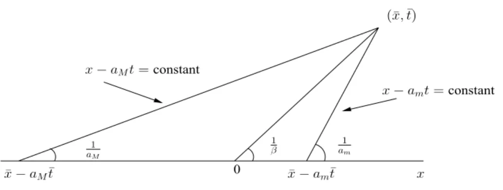
We recall that each realization A(ω) yields the random function (x,t) →
U0(x−A(ω)t), i.e., the initial condition atx0=x−A(ω)t. Also, as illustrated in Figure 1, for a fixed(x¯,t¯)we havex¯−aMt¯≤ x0 ≤ ¯x−amt¯.Hence the solu-tion at(x¯,t¯)depends upon the initial data in the interval x¯−aMt¯, x¯−amt¯
. As shown in Figure 1, this interval is determined by two characteristics x− aMt = constant and x −amt = constant, both passing through (x¯,t¯). From now on the intervalx¯ −aMt¯, x¯ −amt¯
will be referred to as theinterval of dependenceof the point(x¯,t¯).
To separate the contributions of the left state,U0−, and right state,U0+, to the
solution at(x¯,t¯), we shall callβ = xt¯¯ and define the following disjoint subsets of[am,aM]:
M−=a; xa= ¯x −at¯<0 and M+=
a; xa = ¯x−at¯>0 .
Comparing the slopes of the characteristics (see Figure 1), we can rewrite these sets as
M− =
a; 1
aM ≤
1
a <
1 β
= {a; β <a≤aM} and
M+ =
a; 1
β < 1
a ≤
1
am
constant
0
constant
Figure 1 – Interval of dependence.
Thus, the probability of occurrence of the setsM+andM−can be calculated
using the cumulative probability function of the velocity:
P(M+)= FA(β)=θ and P(M−)=1−FA(β)=1−θ. (6)
The solution to (5) is given by the following:
Proposition 1. Let(x¯,t¯),t¯>0, be an arbitrary point andβ = xt¯¯. The solution to(5)at(x¯,t¯)is the random variable
U(x¯,t¯)=(1−X)U0−+XU0+=U0−+XU0+−U0−, (7) where X is the Bernoulli random variable with P(X = 0) = 1−FA(β)and
P(X =1)= FA(β).
Proof. To prove this proposition we use the characteristicsx −amt = 0 and
x −aMt = 0 to divide the semi-planet ≥ 0 into three regions, R1 =(x,t);
x < amt , R2 = (x,t);amt ≤ x ≤ aMt , and R3 = (x,t);x >aMt , and we demonstrate (7) for each one of this regions.
If(x¯,t¯)∈ R2, we may divide the interval of dependence into two sub-intervals: I−=x¯−aMt¯, 0
and I+=0, x¯−amt¯
.
is equal to the probability of occurrence of M−. Thus, from (6) it follows
that P(I−) = P(M−) = 1− F
A(β). Otherwise, in a realization such that
x0 = ¯x −A(ω)t¯ ∈ I+, the contribution will be due only to the right state and we use the same arguments above to conclude that P(I+)= P(M+)=F
A(β). Finally, taking in account the probability of occurrence of U0− and U0+, the
solution is obtained “weighting” their respective probabilities, i.e.,U(x¯,t¯) = (1− X)U0− +XU0+, where X is the Bernoulli random variable with P(X =
1)= FA(β)andP(X =0)=1−FA(β).
If(x¯,t¯)∈ R1thenx¯−amt¯<0 and all the points of the interval of dependence,
¯
x−aMt¯, x¯−amt¯
, are negatives. Therefore, only the left state contributes to the solution, i.e.,U(x¯,t¯)=U0−with probability one. In this case the solution
is (7) with FA(β) = 0. On the other hand, if(x¯,t¯) ∈ R3 only the right state contributes to the solution and we have U(x¯,t¯) = U0+ with probability one,
i.e., (7) withFA(β)=1.
Corollary 1. The solution of(5)is constant along the rays xt =constant, i.e., the random solution is a similarity function.
Proof. This result follows directly from (7) since if xt =constant thenFA x
t
=constant.
Proposition 2. If(x,t)is fixed,n ∈N,n ≥ 1, and we assume the statistical
independence of Aand bothU0−andU0+, then the nt h moment of the random solution(7)is given by:
Un(x,t)=(U0−)n+FA x
t (U
+
0)n
−(U0−)n . (8)
Proof. From Proposition 1,
U(x,t)=U0−+XU0+−U0−=(1−X)U0−+XU0+, whereX = X(x,t)is the Bernoulli random variable:
X =
1, P(X =1)= FA x
t
=θ
0, P(X =0)=1−FA x
t
It is easy to see thatXj=FA x
t
=θ, for all j =1,2,3, . . ..
To prove (8) we first need the following results:
• For alln≥1,
n
j=0 (−1)j
n j
=0, (9)
where
n j
is the binomial coefficient.
• Forn ≥1 and 1≤ j≤n−1,
(1−X)n−j Xj =
Xj
n−j
m=0 (−1)m
n− j
m
Xm
= n−j
m=0 (−1)m
n− j
m
Xm+j
= n−j
m=0 (−1)m
n− j
m
Xm+j
θ
= θ n−j
m=0 (−1)m
n− j
m
zero by(9)
=0.
(10)
• Forn ≥1,
(1−X)n = n
j=0 (−1)j
n
j
Xj
= 1+ n
j=1 (−1)j
n j Xj θ
= 1+θ n
j=1 (−1)j
n j
−1by(9)
=1−θ.
Now, assuming the independence of Aand bothU0−andU0+, we have:
Un(x,t) = (1−X)U0−+XU0+n
= n
j=0 n
j
(1−X)n−jXjU0−n−jU0+j
= (1−X)n
1−θby(11)
U0−n+Xn
θ
U0+n
+ n−1
j=1
n j
(1−X)n−jXj
zero by(10)
U0−n−jU0+j
= (1−θ )U0−n+θU0+n.
Corollary 2. For a fixed(x,t),θ =FA x
t
, and considering the independence ofAand bothU0−andU0+, the mean of the solution(5)is
U(x,t) =(1−θ )U0− +θU0+ = U0− +θU0+ − U0−, (12) and the variance is
V ar[U(x,t)] = V ar[U0−] +θV ar[U0+] −V ar[U0−]
+θ (1−θ )U0+ − U0−2.
(13)
Proof. The expression (12) follows from (8) withn =1. On the other hand,
V ar[U(x,t)] = U2(x,t)− U(x,t)2
= (U0−)2+θ(U0+)2−(U0−)2 −U0−+θU0+−U0− 2 =
(U0−)2
+θ
V ar[U0+] +U0+2−V ar[U0−] −U0−2
−U0−2 − 2θU0− U0+−U0−−θ2U0+2−2U0− U0++U0−2
= V ar[U0−] +θV ar[U0+] −V ar[U0−] +θU0+2−θU0−2 + 2θU0−2−θ2U0+2−θ2U0−2−2θU0− U0++2θ2U0− U0+ = V ar[U0−] +θV ar[U0+] −V ar[U0−]
+ (θ−θ2)U0+2+(θ−θ2)U0−2−2(θ−θ2)U0− U0+
= V ar[U0−] +θV ar[U0+] −V ar[U0−] +θ (1−θ )U0+ − U0−2.
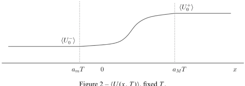
As an illustration we plot in Figure 2 the mean of the solution at a timet =T,
U(x,T), using (12). We can observe a diffusive behavior in the interval [amT, aMT] called by some authors the mixing zone. In this mixing zone U(x,T) is the mean of the left state added to the product of the cumulative probability function of the velocity and the jump between the means of right and left states. This illustration also shows that the shape of the cumulative proba-bility function ofAcontrols the mixing zone: only symmetric density functions
will produce antisymmetrical mixing zones. Our computational tests will make clear this remark (see Figures 3-4 (symmetric) and Figures 5-6 (nonsymmetric)).
Figure 2 –U(x,T), fixedT.
The length of this mixing zone is studied by some authors (see [1, 3, 11, 12], for example) using the effective equation methodology. For instance, the effec-tive equation for the linear transport with random velocity,ν(x), is
∂c
∂t + ν
∂c
∂x −D(t)
∂2c
∂x2 =0,
with the dissipation coefficient given by
D(t)= ! t
0
δν(x −st)δν(x)ds.
If the random velocity is constant then
D(t)= ! t
0
We shall confront a particular solution of the effective equation methodology with our expression for the mean, (12). If we take the initial condition
c(x,0) =U0(x)=
1, x <0, 0, x >0,
for both the effective equation and problem (5), we can show that the analytical expressions for the mean are:
(i) using the effective equation:
c(x,t) = 1 2
1−√2
π ! x−νt
l(t)
0
e−ω2 dω "
,
where l(t)=2#0t D(ω)dω 12
is the mixing length;
(ii) using (12) with a normally distributed random velocity, A=N(ν, σ ):
U(x,t) = 1 2
1−√2
π ! x√−2σtνt
0
e−ω2 dω "
.
Confronting these expressions, they will be equal only if the mixing length satisfiesl(t) = √2σt or, equivalently, if the diffusion coefficient of the
ef-fective equation is D(t) = σ2t, i.e., the same dissipation coefficient for the
constant velocity case.
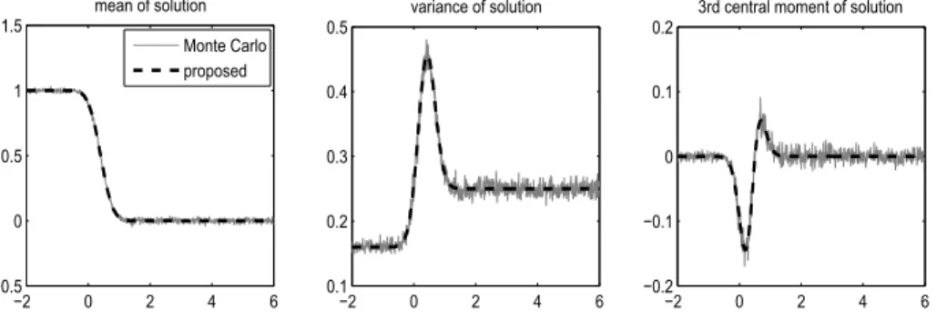
3 Monte Carlo simulations
To assess our results we compare the expressions for the mean, variance and 3rd central moment with Monte Carlo simulations. We use suites of realizations of A, U0− andU0+ considering: the independence of A and bothU0− andU0+;
U0− andU0+ have a bivariate normal distribution with U0− = 1, U0+ = 0, V arU0− = 0.16, V arU0+ = 0.25 and CovU0−,U0+ = 0.12. We plot
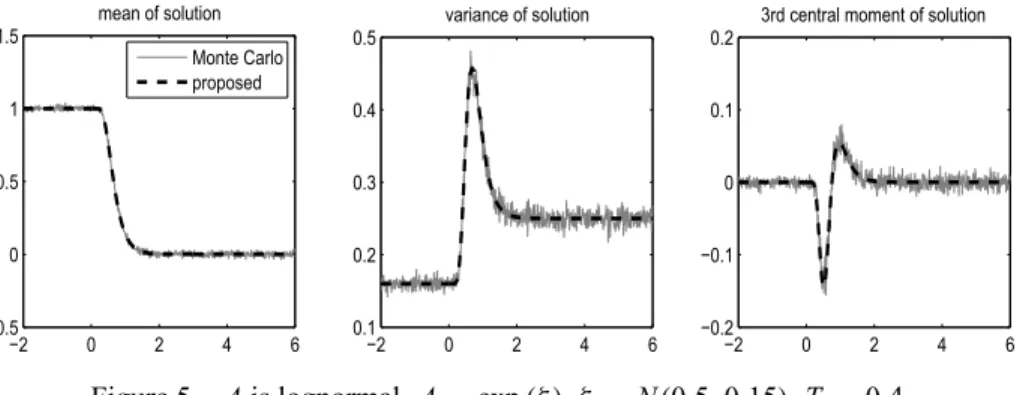
the results in T = 0.4 and T = 0.8. In order to investigate the influence
of the velocity randomness we use two models: (i) A is normally distributed, A = N(1,0.6), in Figures 3 and 4; (ii) A is lognormally distributed, A =
−2 0 2 4 6 −0.5
0 0.5 1 1.5
mean of solution
Monte Carlo proposed
−2 0 2 4 6
0.1 0.2 0.3 0.4 0.5
variance of solution
−2 0 2 4 6
−0.2 −0.1 0 0.1 0.2
3rd central moment of solution
Figure 3 – Ais normal,A=N(1,0.6),T =0.4.
−2 0 2 4 6
−0.5 0 0.5 1 1.5
mean of solution
Monte Carlo proposed
−2 0 2 4 6
0.1 0.2 0.3 0.4 0.5
variance of solution
−2 0 2 4 6
−0.2 −0.1 0 0.1 0.2
3rd central moment of solution
Figure 4 – Ais normal,A=N(1,0.6),T =0.8.
were performed with 1500 realizations and recalling that the solution to (5), at (x,t), for a single realizationA(ω), U0−(ω), U0+(ω)ofA, U0−, U0+, is
U(x,t)=U0(x −A(ω)t)=
U0−(ω), x −A(ω)t <0,
U0+(ω), x −A(ω)t >0.
All the numerical experiments presented in this section were computed in double precision with some MATLAB codes on a 3.0Ghz Pentium 4 with 512Mb of memory.
Concluding remarks
−2 0 2 4 6 −0.5
0 0.5 1 1.5
mean of solution
Monte Carlo proposed
−2 0 2 4 6
0.1 0.2 0.3 0.4 0.5
variance of solution
−2 0 2 4 6
−0.2 −0.1 0 0.1 0.2
3rd central moment of solution
Figure 5 – Ais lognormal,A=exp(ξ ),ξ =N(0.5,0.15),T =0.4.
−2 0 2 4 6
−0.5 0 0.5 1 1.5
mean of solution
Monte Carlo proposed
−2 0 2 4 6
0.1 0.2 0.3 0.4 0.5
variance of solution
−2 0 2 4 6
−0.2 −0.1 0 0.1 0.2
3rd central moment of solution
Figure 6 – Ais lognormal,A=exp(ξ ),ξ =N(0.5,0.15),T =0.8.
be useful in the development of numerical procedures for more general random partial differential equations. Expression (7) shows us that if the statistics of the velocity is known then the local behavior of the solution is independent of the physical mechanisms governing the process. The procedure also shows agreement with the effective equation methodology when the velocity is a normal random variable; however, it seems to us that the random expression to the solution yields more information about the process.
REFERENCES
[1] F. Furtado and F. Pereira,Scaling analysis for two-phase immiscible flow in heterogeneous porous media. Computational and Applied Mathematics,17(3) (1998), 237–263.
[2] J. Glimm,Solutions in the large for nonlinear hyperbolic systems of equations.Comm. Pure Appl. Math.,18(1965), 695–715.
[3] J. Glimm and D. Sharp,Stochastic partial differential equations: Selected applications in continuum physics. In Stochastic Partial Differential Equations: Six Perspectives, (Edited
by R.A. Carmona and B.L. Rozovskii), American Mathematical Society, Providence (1998), pp. 03-44.
[4] S.K. Godunov,A difference method for numerical calculation of discontinuous solution of the equations of hydrodynamics.Mat. Sb.,47(1959), 271–306.
[5] P.E. Kloeden and E. Platen, Numerical Solution of Stochastic Differential Equations.
Springer, New York (1999).
[6] R.J. LeVeque,Finite Volume Methods for Hyperbolic Problems.Cambridge University Press, Cambridge (2002).
[7] B. Oksendal,Stochastic Differential Equations: an introduction with applications.Springer, New York (2000).
[8] H. Osnes and H.P. Langtangen,A study of some finite difference schemes for a uni-diretional stochastic transport equation. SIAM Journal on Scientific Computing,19(3) (1998), 799–
812.
[9] K. Sobczyk,Stochastic Wave Propagation. Elsevier-PWN Polish Scientific Pub., New York (1985).
[10] T.T. Soong,Random Differential Equations in Sciences and Engineering. Academic Press,
New York (1973).
[11] Q. Zhang,The asymptotic scaling behavior of mixing induced by a random velocity field.
Adv. Appl. Math.,16(1995), 23–58.