UNIVERSIDADE DA BEIRA INTERIOR
Ciências Sociais e Humanas
Are Renewable Energy Policies Reducing the
Carbon Dioxide Emissions? The Case of Latin
American Countries
Matheus da Costa Koengkan
Dissertação para a obtenção de Grau de Mestre em
Economia
(2.º ciclo de estudos)
Orientador: Prof. Doutor José Alberto Serra Ferreira Rodrigues Fuinhas
Coorientador: Prof. Doutor António Manuel Cardoso Marques
iii
Dedicatória
v
Agradecimentos
Ao meu orientador, o Professor Doutor José Alberto Fuinhas, pela amabilidade e paciência ao longo do processo de pesquisa e realização desta dissertação. À minha família e amigos que me incentivaram nesta aventura académica no estrangeiro e a todos os docentes do Departamento de Gestão e Economia da Universidade da Beira Interior pelos seus ensinamentos.
vii
Resumo
Esta dissertação examina o impacto das políticas de energias renováveis nas emissões
de dióxido de carbono na região da América Latina. Foram analisados, dez países no
período compreendido entre 1991 a 2012, utilizando como metodologia o modelo auto-regressivo, com desfasamentos distribuídos, para decompor o efeito total e as suas repercussões a curto e longo prazo. Foi detetada a presença da dependência transversal, confirmando que estes países compartilham os mesmos padrões espaciais, bem como a presença de heterocedasticidade, correlação contemporânea e autocorrelação de dependência transversal de primeira ordem. Tendo em atenção estas infrações, foi utilizado o estimador dinâmico Driscoll-Kraay, com efeitos fixos, que é robusto a estes fenómenos. De igual modo, se observou que o consumo de energia primária per capita, contribui, tanto a curto como a longo prazo, para o aumento das emissões de dióxido de carbono. A pesquisa comprovou que o número de políticas e a geração a geração de energias renováveis contribuem para mitigar as emissões de dióxido de carbono.
Palavras-chave
América latina, Dióxido de carbono, Políticas de energias renováveis, Autocorrelação de dependência transversal.
ix
Resumo Alargado
A queima de combustíveis fósseis para a produção de energia tem levado a um aumento nas emissões de dióxido de carbono (CO2). Esse incremento tem causado
uma grande preocupação em todo mundo, tanto no âmbito político como no social. Mais de 80% das emissões de CO2 são causadas pela ação humana, onde a queima de
carvão representa 44% das emissões, o petróleo 36% e o gás natural 20%. Tendo em consideração estes fatores alarmantes, diferentes políticas têm sido aplicadas de forma progressiva para promover o desenvolvimento de fontes de energia renováveis (RES), com o objetivo de reduzir as emissões de CO2. Tendo em atenção as medidas
anteriormente referidas, a América Latina assumiu um papel de grande relevância na promoção das energias renováveis devido ao seu rápido crescimento na implementação das RES, bem como pela abundância de recursos naturais, embora esta promoção apenas se tivesse iniciado na década de 1970 com o choque do petróleo e o posterior impulsionamento das primeiras políticas pró-RES. O primeiro país da América Latina a implementar políticas de energias renováveis foi o Brasil, tendo sido estabelecido em 1975 o programa ProÁlcool, destinado à produção de biocombustíveis. Posteriormente, em 1976 na Costa Rica foi criada a lei para produção de energia de origem geotérmica, um recurso abundante naquele país e por último em 1977 a Nicarágua, seguindo os passos da Costa Rica, estabeleceu também diretrizes para a viabilização da produção de energia geotérmica. Entretanto, o aumento das políticas pró-RES na América Latina está relacionado a uma série de desafios energéticos que a região enfrenta como: (i) a necessidade de aumentar a quantidade substancial de produção de eletricidade a fim de atender o crescimento da demanda; (ii) a falta de diversificação da matriz energética; (iii) a grande exposição dos países Latino Americanos a instabilidade dos preços dos combustíveis fósseis uma vez que esta instabilidade poderia afetar fortemente os orçamentos nacionais e os contratos de fornecimento de eletricidade existentes. Outros fatores podem ser destacados como: Variabilidade do clima, incluindo secas, o que afetam países com grande dependência de energia hidráulica, a infraestrutura precária e envelhecida e por último a necessidade de obtenção de recursos financeiros disponibilizados através de negociações internacionais sobre o clima. No entanto, na América Latina existe uma vasta gama de mecanismos a fim de impulsionar o crescimento da RES como: (i) Metas nacionais de energias renováveis; (ii) Leilões; (iii) Feed-in Tariffs (FITs); (iv) Sistema de certificação; (v) Medição líquida e
Auto-x
suprimento; (vi) Fundos; (vii) Incentivos fiscais; (viii) Acesso à energia renováveis; (ix) Mandos de mistura de biocombustíveis; (x) Mandatos solares; e (xi) Requisitos de conteúdo local. Contudo, na literatura existem poucas pesquisas que abordam o impacto das políticas de energias renováveis nas emissões de CO2. No entanto, em
pesquisas já existentes as políticas mais usadas são: (i) Impostos sobre o carbono; (ii) Feed-in Tariffs; (iii) Pagamentos de prémios; (iv) Sistemas de quotas; (v) Leilões; (vi) Sistemas de capitais, e (vii) Sistemas de comércio. Além disso, há evidências na literatura que estas políticas têm incentivado o aumento das RES e contribuído para a redução das emissões de gases de efeito estufa. Sendo o objetivo desta dissertação, examinar o impacto das políticas de energias renováveis nas emissões de CO2 na
região da América Latina, para atingir tal propósito, na realização desta análise foram abordados dez países Latino Americanos: Argentina, Bolívia, Brasil, Chile, Colômbia, Equador, México, Nicarágua, Peru, e Uruguai, no período compreendido entre 1991 e 2012. Foram utilizadas as seguintes variáveis: (i) Produto Interno Bruto (PIB); (ii) Geração de energias renováveis; (iii) Emissões de dióxido de carbono (CO2);
(iv) Consumo de energia primária; (v) Políticas de energias renováveis. As variáveis escolhidas, seguiram os seguintes critérios: (i) as políticas de energias renováveis têm que ser de longo prazo; (ii) existir dados disponíveis para todo o período em análise. Todas as variáveis em estudo, foram transformadas em per capita exceto as políticas de energia renovável. A opção de utilizar os valores per capita, é justificável pois permite controlar as disparidades de crescimento populacional entre os países. De modo a acomodar a dinâmica esperada entre variáveis, foi utilizado o modelo (ARDL) permitindo assim gerar estimativas de parâmetros consistentes e eficientes, bem como a inferência de parâmetros com base no padrão de teste. De forma a validar o modelo foram feitos testes preliminares como: (i) Dependência Transversal (CSD); (ii) Teste de Raiz de Unidade de Segunda Geração (CIPS); e (iii) Teste de Fator de Inflação de Variância (VIF), e para a especificação do modelo foram utilizados: (i) teste de Wald modificado; (ii) teste de Pesaran; (iii) teste de multiplicador de Langrarian de Breusch e Pagan; (iv) teste de Wooldridge; (v) estatística de Durbin-Watson; (vi) Teste de Baltagi-Wu LBI. Contudo, ao realizar as análises foi detectada a presença de heterocedasticidade, correlação contemporânea, autocorrelação de dependência transversal de primeira ordem. Tendo em atenção estas violações, foi utilizado o estimador dinâmico Driscoll-Kraay, com efeitos fixos, que é robusto a estes fenómenos. De igual modo, se observou que o consumo de energia primária per capita, contribui, tanto a curto como a longo prazo, para o aumento das emissões de dióxido de carbono. A pesquisa comprovou que o número de políticas de energias
xi
renováveis a longo prazo e a geração de energias renováveis contribuem para mitigar as emissões de dióxido de carbono.
xiii
Abstract
This dissertation examines the impact of renewable energy policies on carbon dioxide emissions in Latin America region. Ten countries were analyzed in a period from 1991 to 2012, utilizing the methodology of autoregressive panel with distributed lag to decompose the total effect in their repercussions in the short- and long-run. The presence of cross-sectional dependence confirms that Latin American countries share spatial patterns, as well as, the heteroskedasticity, contemporaneous correlation, and first order autocorrelation cross-sectional dependence were identified. Considering this violations, the robust dynamic Driscoll-Kraay estimator with fixed effects that is robust to these phenomena was used. In the same way, it was observed that the primary energy consumption per capita contributes in both the short- and long-run, to increase in carbon dioxide emissions. The research proved that the number of renewable energy policies in the long-run, and renewable electricity generation per capita both in the short-and long-run, contribute to mitigate per capita carbon dioxide emissions.
Keywords
Latin America, CO2 Emissions, Renewable Energy Policies, Panel Autoregressive
xv
Contents
1 Introduction 1
2 Literature Review 3
2.1 An Overview of Renewable Energy Policies 3
2.2 Renewable Energy Policies in Latin America 5
National Renewable Energy Targets 5
Auctions 6
Feed-In Tariffs 7
Certificate Systems 7
Net Metering and Self-Supply 7
Direct Funds 8
Fiscal Incentives 9
Renewable Energy Grind Access 9
Biofuel Blending Mandates 9
Solar Mandates 10
Local Content Requirements 10
2.3 The CO2 Emissions in Latin America 12
The CO2 Emissions by Sector 13
The CO2 Emissions by Country 14
2.4 The Economic and Political Shocks in Latin America 14
3 Data and Model Specification 17
3.1 Data 17 3.2 Model Specification 19 3.3 Preliminary Tests 19 4 Results 23 5 Robustness Check 27 6 Discussion 29 7 Conclusions 31 References 33 Appendix 39 Annex 41
xvi
List of Figures
Figure 1. Renewable energy policies in Latin America 11
Figure 2. GDP vs. CO2 emissions 12
Figure 3. Sector composition of total CO2 emissions in 2012 13
xix
List of Tables
Table 1. Summary of literature review 3
Table 2. The Latin America renewable energy targets 6
Table 3. Direct funds for renewable energy in Latin America 8
Table 4. Biofuel blending mandates in Latin America 10
Table 5. Variables description and summary statistics 18
Table 6. VIF test and Pesaran CD test 20
Table 7. Unit root tests 21
Table 8. Westerlund cointegration tests 23
Table 9. Estimation results 24
Table 10. Estimation results with shocks 27
Table A1. An example of calculating the variable LPOL 39
Table A2. Renewable energy auctions in Latin America 41
xxi
List of Acronyms
ADF Augmented Dickey Fuller
ARDL Autoregressive Distributive Lag
AR Argentina
BCG Boston Consulting Group
BRA Brazil
BTU British Thermal Unit
BOL Bolivia
BHU Banco Hipotecario del Uruguay (Public Mortgage Bank of Uruguay)
BNDES Banco Nacional de Desenvolvimento Econômico e Social
CCS Carbon Capture and Storage
CDE Conta de Desenvolvimento Energético
CDC Crédito Direto ao Consumidor
CIPS Second-Generation Unit Root Test
CO2 Carbon Dioxide Emissions
CSD Cross-Section Dependence
CHL Chile
COL Colombia
D Differences
DFE Dynamic Fixed Effects
DFE D.-K Dynamic Fixed Effects with Driscoll and Kraay
ECM Error Correction Model
ECU Ecuador
EIA Energy Information Administration
EViews Data Analysis and Statistical Software
FE Fixed Effect
FITs Feed-in-Tariffs
FENOGE Fondo de Energías No Convencionales y Gestión Eficiente de la Energía
FAZNI Fondo de Apoyo Financiero para la Energización de las Zonas No Interconectadas
FEISEH Fondo Ecuatoriano de Inversión en los Sectores Eléctrico e
Hidrocarburífero
xxii
FODIEN Fondo para el Desarrollo de la Industria Eléctrica Nacional
FONER Fondo Nacional de Electrificación Rural
GDP Gross Domestic Product
GWs Gigawatts
GWh Gigawatt-hours
GHG Global Greenhouse Gas
GENREN Programa de Generación Eléctrica a partir de Fuentes Renovables
IEA International Energy Agency
IFM International Monetary Fund
IPPS Independent Power Producers
IRENA International Renewable Energy Agency
L Logarithm
LAC Latin America and Caribbean
LCU Local Currency Unity
LM Lagrangian Multiplier
LLC Levin, Lin and Chu Test
MG Mean Group
MWs Megawatts
MEX Mexico
NIC Nicaragua
PER Peru
PMG Pooled Mena Group
PROALCOOL Programa Nacional do Alcool
PROEOLICA Wind Energy Emergency Program in Brazil
PROINFA Programme of incentives for Alternative Electricity Sources in Brazil PRORENOVA Support for renewal/expansion of sugarcane fields in Brazil
PROESCO Apoio a projetos de eficiência energética
PPA Power Purchase Agreement
RE Random Effects
R&D Research and Development
RES Renewable Energy Sources
RES-E Electricity from Renewable Energy Sources
RPS Renewable Portfolio Standards
REPC Renewable Energy Production Credit
RGR Global Reversion Reserve of Brazil
xxi
URY Uruguay
SENER Secretaria de Energía
STATA Data Analysis and Statistical Software
UECM Unrestricted Error Correction Model
VIF Variance Inflation Facto
VAT Value Added Tax
1
1 INTRODUCTION
The increasing of carbon dioxide emissions (CO2) level have set off an alarm
signal worldwide, causing major concern in the political context and in society in general (Arce et al., 2016). The Latin American countries have seen major increases in CO2 emissions, which have more than doubled during the last three decades
(Al-Mulali et al., 2015). In 2010, the region accounted for about 11% of Global Greenhouse Gas (GHG) (Vergara et al., 2013). Despite this continuous increase, the Latin America region is a small contributor to the world’s GHG (Schipper et al., 2011), but must still be an active player in combating climate change. The policymakers face the dilemma of how to pursue the development of their economies without substantially damaging the environment. Therefore, it is essential that policy makers develop measures to attain economic growth while mitigating climate change (Sakamoto and Managi, 2016). Consequently, several countries have attempted to implement a policy mix of decreasing fossil fuel consumption, while increasing the deployment of renewable energy, with the goal of reducing CO2 emissions (Sakamoto
and Managi, 2016). Europe, as well as in other regions like Latin America has adopted policies to promote renewable energy sources (RES). The renewable energy policies began in the Latin America region in the mid-1970s with the establishment of the ProÁlcool biofuels program in Brazil in 1975, the geothermal laws in Costa Rica in 1976 and Nicaragua in 1977 (IRENA, 2015).
The aim of this dissertation is to answer the following question: Are renewable energy policies reducing the carbon dioxide emissions? To answer this question, the impact of renewable energy policies on CO2, we will analyse emissions
in ten Latin American countries, for the period from 1991 to 2012, using a panel Autoregressive Distributed Lag (ARDL) approach.
In the literature, the impact of renewable energy policies on CO2 emissions
have been scarcely researched. One example is Arce et al. (2016) who investigated whether renewable energy policies, namely carbon taxes, FITs, premium payments, and quota obligations are efficient in reducing CO2 emissions. The authors found that
carbon taxes are the most cost-effective policy for reducing these emissions. Arce and Sauma (2016) analyzed the efficiency of carbon taxes, FITs, premium payments, and quota systems on CO2 emissions. They found evidence that FITs and premium
payments are more cost-effective to reduce CO2 emissions than carbon taxes and
2
payments in RES consumption in Spain and found that the use of premium payments implies a positive externalities valued at 493 million euros for avoided CO2 emissions.
Additionally, based on the results it was identified in the literature review, our central hypothesis that renewable energy policies can mitigate CO2 emissions.
The dissertation addresses the impact of renewable energy policies on CO2 emissions
to identify if these policies are efficient, and makes a contribution to expanding the scarce research regarding these impacts on Latin American countries. The choice of Latin American countries have the attraction of being a region that:
(i) Has experienced rapid growth in renewable energy investment and is very interested in developing those resources:
(ii) Has been a pioneer in designing and implementing specific RES promotion mechanisms;
(iii) Has been an important player in the innovation and development of renewable energy policies.
The dissertation is organized as follows. Section 2, presents the main studies that address the impact of renewable energy policies on CO2 emissions, the
framework of renewable energy policies in the Latin America region, the context of CO2 in the region, and the economic and political shocks in Latin America. Section 3,
presents database use, the model specification, and preliminary tests. Section 4, presents the results. Section 5, presents the robustness check. Section 6, the discussions. Finally, Section 7 presents the conclusions.
3
2 LITERATURE REVIEW
This section is divided into three parts. In the first shows the main studies that address the impact of renewable energy policies on CO2 emissions. The second
shows the framework of renewable energy policies in the Latin America region. The third evidence the context of CO2 in the Latin America region, addressing the
behavior of CO2 emissions in the region, as well as the sectors and countries that
most pollute. Finally, the Fourth shows the economic and political shocks that impacted the Latin America region.
2.1 An Overview of Renewable Energy Policies
The impact of renewable energy policies on CO2 emissions have been barely
researched in the literature. The studies of renewable energy policies have been centred in seven policies (e.g. Arce et al., 2016; Verma and Kumar, 2013) specifically: (i) Carbon taxes; (ii) Feed-in tariffs; (iii) Premium payments; (iv) Quota systems; (v) Auctions; (vi) Cap systems, and (vii) Trade systems. There are evidences in the literature that these policies have paved the way for RES, and helped to restrain CO2 emissions.
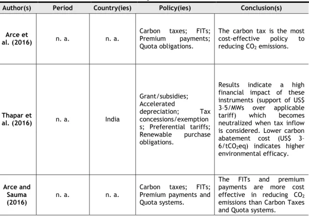
Table 1 presents a summary of the literature review, the namely authors, periods, countries, policies, and main conclusions.
Table 1. Summary of literature review
Author(s) Period Country(ies) Policy(ies) Conclusion(s)
Arce et
al. (2016) n. a. n. a.
Carbon taxes; FITs;
Premium payments;
Quota obligations.
The carbon tax is the most cost-effective policy to reducing CO2 emissions. Thapar et al. (2016) n. a. India Grant/subsidies; Accelerated depreciation; Tax concessions/exemption s; Preferential tariffs; Renewable purchase obligations.
Results indicate a high financial impact of these instruments (support of US$ 3–5/MWs over applicable
tariff) which becomes
neutralized when tax inflow is considered. Lower carbon abatement cost (US$ 3– 6/tCO2eq) indicates higher environmental efficacy.
Arce and Sauma
(2016) n. a. n. a.
Carbon taxes; FITs; Premium payments and Quota systems.
The FITs and premium payments are more cost effective in reducing CO2 emissions than Carbon Taxes and Quota systems.
4
Redondo and Collado
(2014)
2011 Spain Premium payments
The use of premium
payments implies positive externalities valued at 493 million euros in terms of avoided CO2 emissions. Ortega et
al. (2013) 2002-2011 Spain FITs
The FITs encourage the use of RES and the reduction of CO2 emissions.
Verma and Kumar (2013)
n. a. n. a. Carbon quotas; Cap-and-trade and bilateral IPPs.
All policies contribute to reduction of CO2 emissions.
Stokes
(2013) 1997-2012 Canada FITs
The FITs can reduce the cost of renewable energy, and
speed deployment, supporting much-needed decarbonisation. Hinrichs-Rahlwes (2013) 1998-2009 Germany FITs
Mitigate climate change in the best possible way. Green et
al. (2007) n. a. n. a. Carbon Taxes
The carbon tax policies could help to reduce CO2 emissions associated with conventional energy. Wüstenha
gen and Bilharz (2006)
1973-2003 Germany FITs This policy contributes to reduction of greenhouse gases emissions. Palmer and Burtraw (2005) n. a. n. a. REPC and RPS
The RPS policies appear to be more cost-effective than
REPC policies in both
promoting renewables and reducing carbon.
Notes: n. a. denotes ‘not available’. The abbreviations are as follows: Feed-in tariffs (FITs); Renewable Energy Production Credit (REPC); Renewables Portfolio Standard (RPS); Independent Power Producers (IPPs); Carbon Dioxide Emissions (CO2); Renewable Energy Sources (RES); Megawatts (MWs).
The literature provides evidence that premium payments, quota systems, cap systems and trade systems, i.e. all renewable energy policies have opened the way for renewable energy, and have contributed to the mitigation of greenhouse gas emissions.
The following section will highlight the most common renewable energy policies in Latin American countries, as well as the main findings of the literature.
5
2.2 Renewable Energy Policies in Latin America
The fast growth of renewable energy policies seen in Latin American countries could be attributed to the interrelated energy challenges they faced. The region will need a substantial amount of new electricity generation to meet growth in demand, and replace aging infrastructure (Jacobs et al., 2013). Currently, several countries in the Latin America region have energy mixes which expose them to fossil fuel price instability. This could significantly affect their national budgets with pass-through provisions in electricity supply contracts or climate variability (including droughts), especially those with heavy hydro-power structures (Jacobs et al., 2013). These energy challenges have led to an increased interest in the development of RES in Latin American countries.
The renewable energy policies in these countries began in the mid-1970s (IRENA, 2015) with the establishment of: (i) The ProÁlcool biofuels program in Brazil in 1975; (ii) Geothermal laws in Costa Rica in 1976; (iii) Assessment of geothermal resources in Nicaragua in 1977, with the “Master Plan for Electrical Development 1977-2000”. From this initial period, a range of different mechanisms emerged that drove growth in the renewable energy market. The most common mechanisms on the region according to IRENA (2015) are: (i) National renewable energy targets; (ii) Auctions;(iii) Feed-in Tariffs; (iv) Certificate systems; (v) Net metering and self-Supply; (vi) Direct funds; (vii) Fiscal incentives; (viii) Renewable energy grind access; (ix) Biofuels blending mandates; (x) Solar mandates; and (xi) Local content requirements.
The next section will show evidence of the most common renewable energy policies and their operations in the Latin America region.
National Renewable Energy Targets
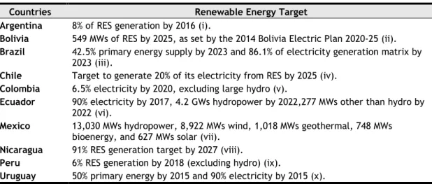
The national renewable energy targets demonstrate the level of RES development and life envisioned by the governments. The RES targets can be applied to electricity, transport sectors and others (Norton Rose Fulbright, 2016). Therefore, many countries in Latin America region have also established their own formal RES targets either by the legislation or decrees (see Table 2).
6
The RE targets have been recognized in all countries in study (see Table 2), with the majority designated to the electricity sector. The RE targets can be based on capacity (MW) or generation (MWh) terms. There are many types of RE targets (e.g. timeline, scope, and technology). For example, Mexico has a targets for RES production of 13,030 MWs hydropower, 8,922 MWs wind, 1,018 MWs geothermal, 748 MWs bioenergy, and 627 MWs solar (Ministerio de Minas e Energía, 2013), while Ecuador has targets of 4.2 GWs hydropower by 2022, 277 MWs other than hydro by 2022 (Consejo National de Electricidad, 2013).
Auctions
The auctions are common policy to the deployment of RES in Latin America region. This policy refers to competitive bidding processes for electricity, where the project developer tale part in the action submit a bid with a price per unit electricity that they are able to realize the project. The government analyses the proposals on the basis of the price and other criteria and signs a contract with winners which offer reliable capacity at efficient prices (Moreno et al., 2010).
In the Latin America region was identified 34 auctions (see Table A2), where the renewable energy-specific (or in that one or more RE technologies were eligible) providing information on the auction year, eligible technologies, amounts auctioned or awarded.
Table 2. The Latin America renewable energy targets
Countries Renewable Energy Target
Argentina 8% of RES generation by 2016 (i).
Bolivia 549 MWs of RES by 2025, as set by the 2014 Bolivia Electric Plan 2020-25 (ii). Brazil 42.5% primary energy supply by 2023 and 86.1% of electricity generation matrix by
2023 (iii).
Chile Target to generate 20% of its electricity from RES by 2025 (iv). Colombia 6.5% electricity by 2020, excluding large hydro (v).
Ecuador 90% electricity by 2017, 4.2 GWs hydropower by 2022,277 MWs other than hydro by 2022 (vi).
Mexico 13,030 MWs hydropower, 8,922 MWs wind, 1,018 MWs geothermal, 748 MWs
bioenergy, and 627 MWs solar (vii). Nicaragua 91% RES generation target by 2027 (viii).
Peru 6% RES generation by 2018 (excluding hydro) (ix).
Uruguay 50% primary energy by 2015 and 90% electricity by 2015 (x).
Notes: The abbreviations are as follows: Gigawatts (GWs); Megawatts (MWs). Sources: Argentina - Boletín Oficial de la Republica Argentina (2006); Bolivia - Ministerio de Hidrocarburos & Energia (2014); Brazil - Ministerio de Minas e Enegia (2013a); Chile - Ministerio de Energía (2013); Colombia - Mnisterio de Minas e Energia (2010); Ecuador - Consejo National de Electricidad (2013); Mexico - Secretaria de Energía (SENER) (2008); Nicaragua - Ministerio de Minas e Energía (2013b); Peru - Congreso de la República de Perú (2010); and Uruguay - Ministerio de Industria, Energía y Minería (2008).
7
Feed-In Tariffs
The Feed-in Tariffs are policies that provide guaranteed buy at an often above market price (Norton Rose Fulbright, 2016). The FITs are destined to some small RES producers, where it can account among others to capacity installed, technology, overall cost and electricity prices (Jacobs et al., 2013). In some countries, the use of FITs are projected to a reduction in generation costs.
In the Latin America region, the first country to implement the FITs was Argentina, in 1998, for solar power and the wind, and expanded in 2006 to cover bioenergy, ocean energy, small hydro, and geothermal. In 2000 Ecuador established the FITs for solar and hydro-power plants, in 2001 Brazil with PROEOLICA for wind power, and in 2002 with PROINFA, providing FITs for small hydro-power, wind, and biomass. Nicaragua in 2005 established FITs for run-of-the-river and wind power, and Uruguay in 2010 established a limited FITs for biomass (IRENA, 2015).
Certificate Systems
Mexico and Chile are the only countries with certificate systems in the region of Latin America. Mexico has a clean energy certificate system, and Chile has also a RES. In Chile the quota was of 5% in 2010, but until 2025 it will be expanding each year until it reaches 20%. Mexico, on the other hand, introduced a quota system in 2014, where the quota for clean energy included renewable energy sources, low-carbon technologies, nuclear energy and fossil fuels with Carbon Capture and Storage (CCS) (IRENA, 2015).
Net Metering and Self-Supply
This policy allows consumers to generate their own electricity from RES and inject surplus generation on the grid, and taking in consideration their contractual terms, consumers can be remunerated or compensated in a future with some sort of discounts in energy bills (Franz, 2016). This policy has a specific design regarding remuneration terms, transmissions costs, losses, fiscal regime, connection provisions, and off-site generation and balancing periods. In Brazil, Chile, Colombia, Mexico, and Uruguay are the only countries in the Latin America region with this kind of policies (see Table A3).
8
Direct Funds
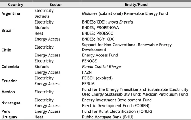
The direct funds are a key for RES developing as well as to achieve other socio-economic benefits such like poverty reduction, energy access, economic development and job creation. In nine Latin American countries have established and defined public funds to promote the development of RES (see Table A2). Table 3 summarizes the identified funds.
Table 3. Direct funds for renewable energy in Latin America
Country Sector Entity/Fund
Argentina Electricity Misiones (subnational) Renewable Energy Fund
Biofuels Brazil
Electricity BNDES;(CDE); Inova Energia
Biofuels BNDES; PRORENOVA
Heat BNDES; PROESCO
Energy Access BNDES; RGR; CDC
Chile Electricity
Support for Non-Conventional Renewable Energy Development
Energy Access Energy Access Fund
Colombia
Electricity FENOGE
Biofuels Fondo Capital Riesgo
Energy Access FAZNI
Ecuador Electricity FEISEH (expired)
Energy Access FERUM
Mexico Electricity Fund for the Energy Transition and Sustainable Electricity Use; Energy Sustainability Fund; Mexican Petroleum Fund
Nicaragua Electricity Energy Investment Development Fund
Energy Access Electric Development Fund (FODIEN)
Peru Energy Access Fund for Rural Electrification (FONER)
Uruguay Heat Public Mortgage Bank (BHU)
Notes: IRENA (2015). Information was adapted by author. The abbreviations are as follows: Banco Nacional de Desenvolvimento Econômico e Social (BNDES); Conta de Desenvolvimento Energético (CDE); Support for renewal/expansion of sugarcane fields in Brazil (PRORENOVA); Apoio a projetos de eficiência energética (PROESCO); Global Reversion Reserve of Brazil (RGR); Crédito Direto ao Consumidor (CDC); Fondo de Energías No Convencionales y Gestión Eficiente de la Energía (FENOGE); Fondo de Apoyo Financiero para la Energización de las Zonas No Interconectadas (FAZNI); Fondo Ecuatoriano de Inversión en los Sectores Eléctrico e Hidrocarburífero (FEISEH); Programa de Energización Rural y Electrificación Urbano-Marginal (FERUM); Fondo para el Desarrollo de la Industria Eléctrica Nacional (FODIEN); Fondo Nacional de Electrificación Rural (FONER); Banco Hipotecario del Uruguay (BHU).
The Direct funding would be in the form of grants, direct contract of provisions of equity or debt and subsidies. The direct funding for RES in other Latin American countries have a direct contracting, where RES projects are awarded contracts through direct negotiation or through by PPAs.
9
Fiscal Incentives
The fiscal incentives for RES have been recognised in nine countries like Argentina, Brazil, Bolivia, Colombia, Ecuador, Mexico, Nicaragua, Peru and finally, Uruguay (see Table A3). The fiscal incentives include the following policies: (i) National Exemption of Local Taxes; (ii) Fuel Tax Exemption; (iii) Import or Export Fiscal Benefit; (iv) Value Added Tax (VAT); (v) Income Tax Exemption; (vi) Carbon Tax; (vii) Accelerated Depreciation; and (viii) Other Fiscal Benefits. In Argentina and Peru, fiscal stability incentives have been implemented with the renewable energy technologies being protected from possible changes in their additional fees and fiscal regime. In some cases, new RE specific taxes are created like concession fees for hydro-power in Argentina, Brazil, Bolivia, Colombia, Peru and Uruguay, and geothermal surface tax and vapour tax in Nicaragua (IRENA, 2015).
Renewable Energy Grind Access
The renewable energy grind access policies have been recognised in seven countries in Latin America: Brazil, Colombia, Ecuador, Mexico, Nicaragua, Peru, and Uruguay (see Table A3). This policy includes: (i) transmission discount or exemption (ii) priority or dedicated transmission; (iii) grind access; (iv) preferential dispatch; and (v) other grind benefits.
In some countries (like Colombia), the RES developers under 20 MWs are exempt form a reliability fee to remunerate for reserve power. In Mexico, the development of renewable energy grind access is dedicated to RES transmissions lines through of a coordination process between the energy regulator, the public utility, and RES producers, while in Peru the renewable energy grind access considerate zones with high RES potential in transmission plans (IRENA, 2015).
Biofuels Blending Mandates
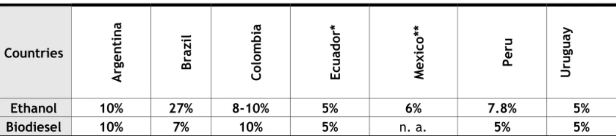
In Latin America region, the policies for the promotion of RES in the transport sector is focussed on the use of biofuels and dominated by blending mandates. These mandates establish a percentage of biofuels (e.g. ethanol or biodiesel) that blended with diesel or gasoline (REN21, 2014). In seven countries have blending mandates in their legislation (see Table 4).
10
Table 4. Biofuel blending mandates in Latin America
Countries A rg e n ti n a B ra zi l C ol om b ia Ec u ad or * M ex ic o* * P er u U ru gu ay Ethanol 10% 27% 8-10% 5% 6% 7.8% 5% Biodiesel 10% 7% 10% 5% n. a. 5% 5%
Notes: n. a. denotes ‘not available’. IRENA (2015). Information was adapted by the author. * Ethanol blend only in Guayaquil; * Only in Guadalajara, Monterrey and Mexico D.F.
The national mandates are applying all territory like Argentina, Brazil, Colombia, Peru and Uruguay or apply only to certain metropolitan areas like in Mexico and Ecuador (see Table 4). The fiscal incentives like the fuel taxes, tax exemption are another integral part of biofuels support policies in some countries in Latin America region like Argentina, Brazil, Colombia, and Uruguay.
Solar Mandates
The solar mandates are policies that establish a percentage of their heating needs (e.g. water heating), through solar energy to commercial buildings, industrial and public facilities (REN21, 2014). The Latin America region has a large and unexploited potential for this kind of policy. The solar mandates usually apply to new constructions. In this region, the countries which encourages the use of solar power are: Mexico, Brazil, Uruguay and Nicaragua (IRENA, 2015).
Local Content Requirements
There are others policies and support aspects that contribute to the enabling condition of RES deployment. In some countries in the region of Latin America like Brazil, Ecuador, and Uruguay, all have a local content requirement like policy (see Table A3). The local content requirement is imposed in several ways like a percentage of investment, hiring of personnel and use of local materials. For example, both Ecuador and Uruguay impose percentages of local staff to the RES plant control. The local content has been used like a percentage of investment in Uruguay is 20%, Ecuador 40 % and in Brazil is 60% (IRENA, 2015).
Indeed, few authors have focused on the analysis of the impact of RES policies on CO2 emissions in Latin American countries. For instance, Pereira et al. (2011)
11
power generation system. Those authors found that the introduction of the energy compensation mechanism had the advantage of being a mechanism that compensated producers to invest in plants emitting less CO2. Jacobs et al. (2013) studied FITs in 12
Latin America and Caribbean (LAC) countries. The results indicated that some LAC countries namely Argentina, Dominican Republic, Ecuador, Honduras, and Nicaragua have used FITs to promote renewable energy to reduce the CO2 emissions, and that
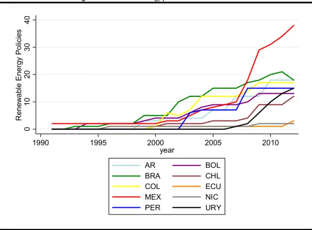
FITs are becoming increasingly popular. If well designed, they can mitigate investor risk in RES. Zwaan et al. (2016) investigated opportunities for energy technology deployment like part of climate change mitigation efforts in Latin American countries. The authors project several renewable energy policy scenarios up to 2050, which could to reduce the CO2 emissions. Figure 1 demonstrates the renewable
energy policies charted by crosses.
As shown by Figure 1 the renewable energy policies are constantly growing in Latin American countries, reinforcing the necessity to study. The next section will show the context of the CO2 emissions in Latin America region.
Figure 1. Renewable energy policies in Latin America
0 10 20 3 0 40 R en ew a bl e E ne rg y P o lic ie s 1990 1995 2000 2005 2010 year AR BOL BRA CHL COL ECU MEX NIC PER URY
Source: Author compilation based on International Energy Agency (IEA) data. Notes: The abbreviations are as follow: Argentina (AR); Brazil (BRA); Chile (CHL); Colombia (COL); Peru (PER); Ecuador (ECU); Uruguay (URY); Bolivia (BOL);Mexico (MEX); Nicaragua (NIC).
12
2.3 The CO
2Emissions in Latin America
The total CO2 emissions in Latin America in 2010 were at 4.7 GtCO2 is (10.8%
of total global emissions). This index represents a decline of 11 % since the start of the century due to the changes related with the reduction in land-use and the ones related with emissions and energy intensity (Vergara et al., 2013)
.
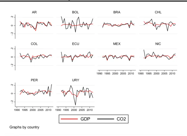
This decrease occurred during a period of increase in the gross domestic product of countries in the Latin America region, where indicates that economic growth has decoupled from emissions (see Figure 2).As shown in Figure 2, the economic growth has decoupled from CO2 emissions
in countries of Latin America region. The decoupling is due to the introduction of new renewable energy sources in the energy mix as well as the introduction of new technologies that emit less CO2.
The next subsections will evidence the main sectors that contribute to CO2
emissions in the analysed region.
Figure 2. GDP vs. CO2 emissions -. 2 0 .2 -. 2 0 .2 -. 2 0 .2 1990 1995 2000 2005 2010 1990 1995 2000 2005 2010 1990 1995 2000 2005 2010 1990 1995 2000 2005 2010 AR BOL BRA CHL
COL ECU MEX NIC
PER URY
GDP CO2
Graphs by country
Source: Author compilation based on International Energy Agency (IEA) and World Bank Data (WBD).Notes: The abbreviations are as follows: Gross Domestic Product (GDP); Carbon Dioxide Emissions (CO2); Argentina (AR); Brazil (BRA); Chile (CHL); Colombia (COL); Peru (PER); Ecuador (ECU); Uruguay (URY); Bolivia (BOL);Mexico (MEX); Nicaragua (NIC).
13
The CO
2Emissions by Sector
The annual emission levels in Latin America region has deteriorated in recent years. The CO2 emissions intensity in the studied region fell from 1.500 (tCO2) per
million dollars of GDP in 1990 to 1.300 (tCO2) per million dollars of GDP in 2005
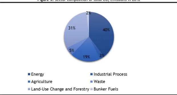
(Vergara et al., 2013). The mainly composed sectors that contribute to GHG emissions in Latin America are: (i) Energy;(ii) Industrial Process; (iii) Agriculture; (iv) Waste; (v) Land-Use Change and Forestry, and (vi) Bunker Fuels. Figure 3 shows the sector composition of total CO2 emissions in Latin America region in 2012.
Figure 3 shows that the 40 % CO2 emissions come from energy consumption,
where in Latin America region the energy matrix is mainly composed by fossil fuels (e.g. Oil 46 %, Natural gas 23 % and Coal 5 %). However, at the same time it is incorporated by renewable sources (e.g. Bioenergy and Waster 16 %, Hydro-power 8%, Geothermal 1%, and Solar, Wind and Others <1 %) (IRENA, 2016).
The second and third greatest contributors to CO2 emissions are land-use
Chand and Agriculture. In contrast to the global picture, the emissions in the region are generated not only from energy use, but from land use, agriculture and forestry. As can be seen in Figure 3, the Land-Use change contributes to 31 % in CO2
emissions, while Agriculture 19 %. The Latin America emissions profile is opposite to the world profile, where 50 % of emissions come from agriculture and land use, and only 39% come from energy.
Figure 3. Sector composition of total CO2 emissions in 2012
Source: Author compilation based in World Resource Institute (WRI) (2017) data. Notes: The above sector contributions refer to percentage shares of total Latin America CO2 emissions.
14
The CO
2Emissions by Country
Most countries in the region of Latin America are small contributors to the CO2
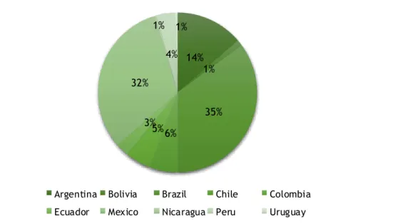
emissions, with emissions representing less than 1 % of the global total. This region includes some very large carbon emitters’ countries that are in a transition process induced by innumerable structural changes. Figure 4 illustrates the relative contributions of these principal countries to the regional emissions profile.
Figure 4. The CO2 emissions by country in 2012
14% 1% 35% 6% 5% 3% 32% 1% 4% 1%
Argentina Bolivia Brazil Chile Colombia
Ecuador Mexico Nicaragua Peru Uruguay
Source: Author compilation based on Energy Information Administration (EIA) data. Notes: The percentage shares of total Latin America CO2 emissions.
Brazil was the dominant source of Latin America emissions 35% in 2012 followed by Mexico 32% and Argentina 14 %. The Latin America region is only globally relevant in terms of CO2 emissions because of Brazil that alone contributes one-third
of global land-use emission and Mexico.
The next section will show the economic and political shocks that impacted the Latin America region.
2.4 The Economic and Political Shocks in Latin America
The Latin American countries suffered several economic and political shocks which have impacted the economic growth of the region. However, during the 1990s and the first half of the 2000s and the years 2008-2009, the region suffered several financial crises. The best known of these are the Mexican crisis of 1994-1995, the Brazilian crisis of 1999, the Argentine crisis of 1999-2002, the Uruguayan crisis of 2002 and the Subprime crisis of 2008-2009. These crises are associated with market reforms and the opening of their economies (Edwards, 2008).
15
The Mexican financial crisis of 1994-1995 refers to the crisis that started after Mexico’s devaluation of the peso in 1994, due to the lack of International reserves This crisis was the worst banking crisis in Mexican history (1994-1997), where the depreciation of the currency in December of 1994 was from about 5.3 Pesos per Dollar to over 10 Pesos per Dollar. In November of 1995, Mexico suffered a severe recession which lasted more than a decade, with a decrease of 6 % of GDP (Musacchio, 2012). Mexican’s crisis impacted the mainly countries of Latin America region like Argentina and Brazil, where both suffered several financial and cambial crisis. This impact was known as “Tequila Effect” in South American region (Aldrighi and Cardoso, 2009).
The Brazilian currency crisis of 1999 is a result of the crisis of Brazilian Real (BRL) and the devaluation of the exchange rate in January 1999. Moreover, this crisis is directly associated with the structural problems of an anti-inflation plan that was implemented in Brazil. The Brazilian Real plan was successful in controlling the inflation in 1994, but the implementation of deflationary economic policies with an overvalued semi-fixed exchange rate led Brazil into a serious structural economic problem (Averbug and Giambiagi, 2000).
The Argentine financial crisis of 2001-2002 started in 1999 due to several internal and external factors. First, the economic decline, due to a high unemployment and fiscal imbalance. Second, due to the Russian crisis in 1998, the devaluation of the Brazilian currency in 1999, and an enormous aversion to the risk of international financial markets. Taking in consideration the above reasons, the Argentine government established in 2001 that the parity of the Peso should be the same as the Dollar, However, this change brought a severe crisis to the convertibility of the Peso (Fernandes, 2003).
The Uruguayan crisis of 2002, occurred during the severe crisis of Peso convertibility which affected Argentina between 2001 and 2002. Many of the country’s customers withdrew their dollar deposits held in Uruguayan banks. This caused a crisis in the financial system in 2002 (Brun and Licandro, 2005).
The subprime crisis of 2008-2009 impacted all countries of Latin America region in different ways, because of the great differences between them. The large and medium-sized countries, already heavily industrialized and urbanized, such like Mexico, Argentina, Colombia, Peru, Venezuela, and Chile, were hit by the crisis in a similar way to Brazil. The principal effects were: foreign exchange flight, exports and external credit, Private banks, which also cut credit and increased interest rates, and as a result the internal market contracted, leading to a fall in production
16
and an increase in unemployment. The small countries like Nicaragua, Bolivia, Ecuador and Uruguay were hit by the international crisis in a more direct way. This impact is due to the fact that these countries are highly dependent of imported products, and have a limited number of primary products to export (Singer, 2009).
The next section will show the used database and specification model while elaborating this dissertation.
17
3 DATA AND METHODOLOGY
This section is divided into three parts. The first one, shows the variables and the used database. The second shows the model specification. The third shows the preliminary tests.
3.1 Data
In the next lines, the available data in renewable energy policies of the last twenty years (1991-2012) will be analysed, taking in consideration ten countries, namely: Argentina, Bolivia, Brazil, Chile, Colombia, Ecuador, Mexico, Nicaragua, Peru, and Uruguay. The selection of these countries was based on the available data for RES generation, CO2 emissions, primary energy consumption, and renewable
energy policies. The used variables are: (i) Carbon dioxide emissions from energy consumption in million metric tons, and transformed in per capita; (ii) Renewable energy consumption in Kilowatt-hours from hydroelectric, geothermal, wind, solar, tide, wave and biomass and transformed in per capita; and (iii) Renewable energy policies that was constructed as follows form: First, the renewable energy followed selection criteria: (i) Renewable energy policies that include following energy sources: Bioenergy, Geothermal, Hydropower, Ocean, and Solar; (ii) Renewable energy sector that include: Electricity, Framework Policy, Heating and Cooling, Multi-sectoral Policy, Transport; (iii) Renewable energy policies jurisdiction that include: International, National, State/Regional, Municipal; (iv) Policy status that include: Just policies with follow status (In Force and Ended), and renewable energy policies that were superseded, under review and planned were excluded from database. Second, were selected the follows policy types availably in IEA for the countries in studies: (i) Economic Instruments that include following policies: (a) Fiscal/financial incentives with: feed-in tariffs/premiums, grants and subsidies loans, tax relief, taxes and User charges; (b) Market-based instruments which have the following policies: GHG emissions allowance, green certificates, white certificates; (c) Direct investments that include following policies: Funds to sub-national governments, infrastructure investments, Procurement rules, RD&D funding); (ii) Information and Education which have the following policies: Advice/Aid in Implementation, Information provision, Comparison label, Endorsement label, Professional training and qualification; (iii) Policy Support that include following policies: institutional creation, strategic planning; (iv) Regulatory
18
Instruments which have the following policies: Auditing; codes and standards, monitoring, obligation schemes, other mandatory requirements; (v) Research, Development and Deployment (RD&D) which have the following policies: Demonstration project, technology deployment and diffusion, technology development; (vi) Voluntary Approaches that include following policies: Negotiated agreements (e.g. Public-private sector), public voluntary schemes, unilateral Commitments (e.g. Private sector). Third, the calculation of variable LPOL is simple and was done as follow: The construction of variable was done by summing of all renewable energy policies types accumulated in the run of their operation, in other words policies (In force and ended), to a better understanding (see, an example in Table A1); (iv) Primary energy consumption in quadrillion Btu from fossil fuels and other sources and transformed in per capita; and (v) Gross domestic product (GDP) in constant local currency unity (LCU) and transformed in per capita.
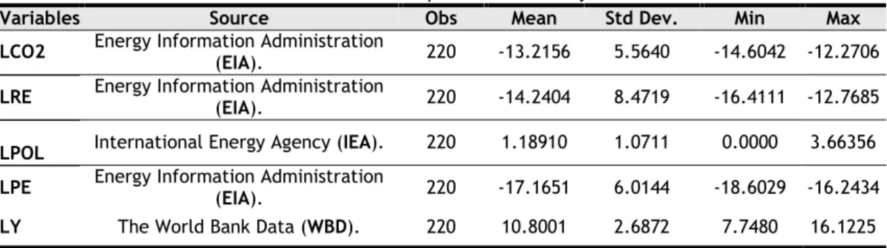
All the variables except the renewable energy policies were transformed in per capita. The use of per capita values let us control the growth of population disparities among the Latin American countries. Hereafter the prefixes, L, and, D, denote natural logarithm, and first differences of the variables, respectively. Table 5 shows the name, definition, source of raw data and summary statistics of the variables.
Given that renewable energy policies are likely to require time to produce their full effect in CO2, an approach with the ARDL model panel was used. The
properties of this estimation method allow the decomposition of the total effect into is short-and long-run dimensions. Accordingly, to achieve the goal of decomposing the global effects in the short-and long-run, we balanced the longest available time span with the maximum possible number of Latin American countries which have renewable energy policies made available. To elaborate the econometric analysis, the EViews 9.5 and Stata 14.2 software were used.
Table 5. Variables description and summary statistics
Variables Source Obs Mean Std Dev. Min Max
LCO2 Energy Information Administration (EIA). 220 -13.2156 5.5640 -14.6042 -12.2706
LRE Energy Information Administration (EIA). 220 -14.2404 8.4719 -16.4111 -12.7685
LPOL International Energy Agency (IEA). 220 1.18910 1.0711 0.0000 3.66356
LPE Energy Information Administration (EIA). 220 -17.1651 6.0144 -18.6029 -16.2434
19
3.2 Model Specification
To analyse the impact of renewable energy policies on CO2 emissions, we used
an unrestricted error correction model (UECM) form of the ARDL model. This model decomposes the total effect of a variable into its short-and long-run components (e.g. Srinivasan et al., 2012). Moreover, this model generates consistent and efficient parameter estimations as well as the inference of parameters based on the standard test. The general UECM form of the ARDL model used in this empirical analysis follow the specification of Equation (1):
2i i t 25i 1 t 24i 1 t 23i 1 t 22i 1 t 21i 1 t k 0 i 25i 1 t k 0 i 24i 1 t k 0 i 23i 1 t k 1 i 22i t i it it LY γ LPE γ LPOL γ LRE γ LCO2 γ DLY θ DLPE θ DLPOL θ DLRE θ TREND θ θ DLCO2
(1)where
it represents the intercept,
i is the trend, iii21,2521 are the estimated parameters and
2iis the error term.3.3 Preliminary Tests
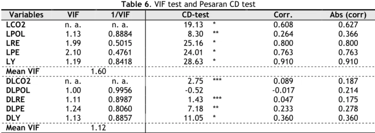
This section shows the preliminary tests in data to check theproperties of the variables. Indeed, considering the macro panel, the best econometric practices strongly recommend testing for the presence of heterogeneity, which could arise when a long time span is used. The long-time spans exacerbate the potential occurrence of a panel with parameter slope heterogeneity and the presence of cross-section dependence (CSD). In Latin American countries, it is expected the existence of CSD in the model,due to some common characteristics shared by these countries. When the presence of CSD is not controlled, it can produce both biased estimates and a severe identification problem (e.g. Eberhardt and Presbitero, 2013) which require appropriate estimators to handle them. The CSD and the order of integration of the variables are analysed to capture the features of both series and crosses. To check for the presence of multi-collinearity, the variance inflation factor (VIF) was applied. This test provides an indication of the impact of multi-collinearity in the accuracy of estimated regression coefficients (e.g. O’Brien, 2007). Table 6 reveals both results of VIF test and the CSD.
20
Table 6. VIF test and Pesaran CD test
Variables VIF 1/VIF CD-test Corr. Abs (corr)
LCO2 n. a. n. a. 19.13 * 0.608 0.627 LPOL 1.13 0.8884 8.30 ** 0.264 0.366 LRE 1.99 0.5015 25.16 * 0.800 0.800 LPE 2.10 0.4761 24.01 * 0.763 0.763 LY 1.19 0.8418 28.63 * 0.910 0.910 Mean VIF 1.60 DLCO2 n. a. n. a. 2.75 *** 0.089 0.187 DLPOL 1.00 0.9956 -0.52 -0.017 0.214 DLRE 1.11 0.8987 1.43 *** 0.047 0.175 DLPE 1.24 0.8060 7.18 ** 0.233 0.278 DLY 1.13 0.8857 11.05 * 0.360 0.360 Mean VIF 1.12
Notes: n. a. denotes ‘not available’. ***, **, * denote statistically significant at 1%, 5% and 10% level, respectively. The Stata command xtcd was used to achieve the results for CSD.
The value of mean of VIF was 1.60 in levels, and at the first differences were 1.12. The low VIF statistics than benchmark 10% support the argument that multi-collinearity is of no great concern in the model. The panel data techniqueallows the heterogeneity control of the crosses. When many individuals are analysed, it provides more information, variability, degrees of freedom and efficiency and thus, less collinearity than is generally present in the time series approach (e.g. Klevmarken, 1989; Hsiao, 2003). The CSD-test points to the presence of cross-section dependence in the variables both in levels and in first differences, except for the RES generation in differences (DLRE). A possible answer for this result is that the generation of RES is largely country-specific and conditional in the intermittence that characterizes its generation (e.g. solar and wind sources). The presence of CSD shows evidence of interdependence between the cross-sections, i.e. that the countries share common shocks.
To assess the order of integration of the variables, the first and second-generation unit root tests were used. The first second-generation unit root tests of LLC (Levin, Lin, and Chu, 2002), ADF-Fisher (Maddala and Wu, 1999), and ADF-Choi (Choi, 2001), were used. The second-generation unit root test CIPS (Pesaran, 2007) was used. Moreover, the null hypothesis of both tests indicate the existence of unit root. Table 7 shows the results of unit root tests.
21
Table 7. Unit roots tests
Variables 1st Generation test 2nd Generation unit root test
CIPS (Zt-bar)
LLC ADF-Fisher ADF-Choi
Individual intercept and trend Without trend With trend
LCO2 -1.0714 24.3974 -0.6699 -0.776 0.969 LRE -4.2044 *** 39.3896 *** -2.6446 *** -1.337 *** -1.300 *** LPOL -0.8576 17.7105 0.1587 -0.404 1.056 LPE -0.5597 27.8676 -1.0734 -0.678 1.259 LY 0.6792 18.9771 1.0888 -1.199 -0.750 DLCO2 -6.7437 *** 83.8301 *** -6.6476 *** -4.976 *** -4.710 *** DLRE -13.0036 *** 139.080 *** -9.6431 *** -6.254 *** -5.157 *** DLPOL -6.0603 *** 65.5947 *** -5.1363 *** -4.038 *** -3.413 *** DLPE -7.3999 *** 113.166 *** -8.0571 *** -3.290 *** -1.868 *** DLY -6.5306 *** 68.1892 *** -5.3035 *** -3.826 *** -2.377 ***
Notes: *** denotes statistically significant at 1% level. The null hypotheses are as follow: LLC test the unit root (common unit root process), this unit root test controls for individuals effects, individual linear trends, has a lag length 1, and Newey-West automatic bandwidth selection and Bartlett kernel were used; ADF-FISHER and ADF-Choi test the unit root (individual unit root process), this unit root test controls for individual effects, individual linear trends, has a lag length 1, the first generation test follows the option “individual intercept and trend”, which was decided after a visual inspection of the series. The EViews 9.5 was used in the calculus of the first generation tests. The CIPS test has H0: series are I(1). The Stata command multipurt was used to compute CIPS test.
The LLC, the ADF and CIPS test (Pesaran, 2007) are consensual, and indicating that all the variables in levels except LRE are integrated of order one I(1), i.e. they have one-unit root. The LRE and all the variables in first differences are stationary. The macro panel structure requires a long time span. This has the advantage of allowing panel unit root tests to have a standard asymptotic distribution, which is essential when checking for cointegration (Baltagi, 2008).
The Hausman test of the RE against the FE specification was applied to identify the presence of RE or FE in the model. This test has the null hypothesis that the best model is RE. The results of Hausman test is statistically significant ( 2 70.03
10
) and indicates the FE model. The presence of FE model in LAM countries
were confirmed by the following authors (e.g. Ferreira et al., 2016; Avelino et al., 2015; Gonçalves, 2013).
This model is appropriate for analyzing the influences of variables over time, as well as to remove all time-invariant features from the independent variables. To check the cointegration of results, we used the second-generation cointegration test of Westerlund (2007). This test has as null hypothesis the existence of no-cointegration between the variables. The Westerlund no-cointegration test is based on an error correction model, where all variables are stationary (Fuinhas et al., 2015).
In the macro panels, the presence of long time spans and many cross-sections, make testing for the slope heterogeneity of parameters highly advisable. This testing could be of two types: (i) heterogeneity of parameters in the short-and long-run, and (ii) heterogeneity of parameters only in the short-run. To deal with heterogeneity, the Mean Group (MG) or Pooled Mean Group (PMG) estimators were applied. The MG
22
is a flexible technique that creates regressions for each individual, and computes to all individuals an average coefficient (Pesaran et al., 1999). This estimator is consistent in the long-run average, while when in the presence of slope homogeneity, the model is not efficient (Pesaran et al., 1999). The PMG is an estimator that in long-run parameter makes restrictions among cross-sections and adjustment speed term. Moreover, this estimator is more efficient and consistent in the existence of homogeneity in the long-run than the MG estimator (Fuinhas et al., 2015).
Finally, a battery of diagnostic tests were performed: (i) Modified Wald test for groupwise heteroskedasticity. This test has the null hypothesis of homoscedasticity; (ii) Pesaran test of cross-section independence, to identify the existence of contemporaneous correlation among cross-sections. The null hypothesis of this test specifies that the residuals are not correlated and it follows a normal distribution; (iii) Breusch and Pagan (1980) Langrarian Multiplier test of independence, that follows chi-square distribution, was performed to measure whether the variances across individuals are correlated; (iv) Wooldridge (2002) test, to check for the existence of serial correlation; (v) Durbin-Watson statistic test, to check the presence of the first-order auto-correlation in the disturbance when all the regressors are strictly exogenous. The null hypothesis of the test is that there is no first-order auto-correlation (Verbeek, 2008, p. 373); and (vi) Baltagi-Wu LBI test, to test serial correlation in the disturbance. The null hypothesis of no first-order serial correlation (Baltagi, 2008, pp. 97-98).
The robustness of the model will be tested with the shocks. Indeed, the residual’s model confirms the existence of shocks that need to be controlled in the following countries: Bolivia, Chile and Uruguay. For this reason, were introduced dummy variables that addressed the following years (BOL2001, URY2001, CHL2007, and URY2009), with the goal to end these distortions, and correct the shocks in the model. The ARDL model is robust to the inclusion of dummies, where the dummies are statistically significant.
23
4 RESULTS
As stated earlier, the aim of this research is to examine the effect of renewable energy policies on CO2 emissions in Latin American countries. It is worth
nothing that the results are based on per capita data. There is evidence of the presence of CSD in the variables (see Table 6). The test of unit roots (see Table 7) point to the possibility of stationary of LRE. Table 8 shows the results of the Westerlund cointegration tests.
Table 8. Westerlund cointegration tests Westerlund cointegration test Statisti
cs None Constant Constant & trend
Value value Z- P-value robust Value value Z- P-value robust Value value Z- P-value robust
Gt -1.777 0.622 0.228 2.547 - -0.337 0.098 -2.484 1.323 0.343
Ga -5.517 1.940 0.088 6.916 - 2.493 0.063 -4.622 4.661 0.466
Pt -5.445 0.263 - 0.116 5.235 - 1.439 0.384 -5.957 2.354 0.406
Pt -5.758 0.154 0.026 5.856 - 1.439 0.111 -4.063 3.609 0.429
Notes: Bootstrapping regression with 800 reps. H0: No cointegration; H1 Gt and Ga test the cointegration for each country individually, and Pt and Pa test the cointegration of the panel as a whole. The Stata command xtwest was used.
The Westerlund cointegration tests rejects the existence of cointegration between variables. The non-detection of cointegration points to the use of econometric techniques that are less stringent, i.e. ARDL models.
The MG and PMG estimators were tested against the dynamic fixed effects (DFE). The robust Driscoll and Kraay (1998) estimator was applied, due to the presence of heteroskedasticity, contemporaneous correlation, first orders auto-correlation and cross-sectional dependence. This estimator is a matrix estimator that generates robust standard errors for several phenomena found in the sample errors. The DFE estimator, DFE robust standard errors, and DFE Driscoll and Kraay were computed. Finally, a battery of specification test like (i) Modified Wald test; (ii) Pesaran test; (iii) Breusch and Pagan Langrarian Multiplier test; (iv) Wooldridge test; (v) Durbin-Watson statistic test; and (vi) Baltagi-Wu LBI test were applied.
Table 9 shows the results of the MG, PMG, DFE estimators, and the outcome of the Hausman test, the semi-elasticities and elasticities of the DFE, DFE Robust and DFE D.-K. Models, and the model specification tests. The semi-elasticities were computed by adding the coefficients of variables in the first differences. The elasticities are computed by dividing the coefficient of the variables by the coefficient of (LCO2), both lagged once and multiplying the ratio by -1.
24
The elasticities have the expected signs and are highly significant. Additionally, in semi-elasticities, the renewable energy policies (DPOL) do not cause any sort of impact over carbon dioxide emissions (DLCO2) in the short-run. The elasticities of renewable energy policies (LPOL) reduce the carbon dioxide emissions (LCO2) to -0.0358 in the long-run. The RES consumption (DLRE) in the short-run reduced the carbon dioxide emissions (LCO2) to -0.1854, and in the long-run they have decreased -0.1965. Additionally, as expected, the primary energy consumption (LPE) and Economic Growth (LY) increased the carbon dioxide emissions (LCO2) in the short and long-run.
The Hausman test indicates that the DFE is the appropriate estimator, i.e. there is evidence that the panel is ‘homogeneous’. The estimations result from the DFE estimator, DFE robust standard errors, and DFE Driscoll and Kraay points to the presence of long memory in the variables. The results are due to the ECM term being statistically significant at 1% level and having a negative sign, where this result confirms the presence of Granger causality (Jouini, 2014).
Table 9. Estimation results (Dependent Variable DLCO2)
Heterogeneous estimator Fixed effects
MG (I) PMG (II) Coefficient FE (III) FE Robust (IV) FE D.-K. (V)
Constant -2.7910 -4.5068 *** -5.2545 *** *** *** Trend -0.0013 -0.0027 ** 0.0006 Short-run (semi-elasticities) DLRE -0.2279 *** -0.1676 *** -0.1854 *** *** *** DLPOL 0.0173 0.0502 0.0061 DLPE 0.8176 *** 0.7630 *** 0.5822 *** *** *** DLY 0.5204 *** 0.5203 *** 0.4276 *** *** *** Long-run (elasticities) LRE(-1) -1.0157 -0.1163 *** -0.1965 *** *** *** LPOL(-1) -0.0414 0.0078 -0.0358 *** *** *** LPE(-1) 2.7717 0.6951 *** 0.7082 *** *** *** LY(-1) -1.2185 0.3588 *** 0.4776 *** *** *** Speed of adjustment ECM(-1) -0.9598 *** 0.6763 *** -0.5850 *** *** ***
Hausman test Specification test
MG vs PMG PMG vs DFE Modified Wald
test Pesaran test Wooldridg e test Durbin-Watson test Baltagi-Wu LBI test 2 11 20.30 2 11 0.00 *** 112 172.31 *** N(0,1) = 4.710 *** 111.466*** F (1,9) = 1.7645 1.8559 Notes: ***, ** denote statistically significant at 1%, and 5% level, respectively; Hausman results for H0: Difference in coefficients not systematic; ECM denotes error correction mechanism; the long-run parameters are computed elasticities; the Stata commands xtpmg, and Hausman (with the sigmamore option) were used; in the fixed effects were used the xtreg, and xtscc Stata commands; for H0 of Modified Wald test: sigma(i)^2 = sigma^2 for all I; results for H0 of Pesaran test: residuals are not correlated; results for H0 of Wooldridge test: no first-order autocorrelation; The Stata command xtregar was used in the Durbin-Watson statistics test and Baltagi-Wu LBI test: The null hypothesis of the Durbin-Watson statistics test is that there is no first-order autocorrelation, and Baltagi-Wu LBI test the null hypothesis of no first order serial correlation.