Proceedings of the 2009 ASME International Mechanical Engineering Congress & Exposition IMECE2009 November 13-19, 2009, Lake Buena Vista, Florida, USA
IMECE2009-11029
DEPENDENCY OF AIR CURTAIN PERFORMANCE ON DISCHARGE AIR VELOCITY
(GRILLE AND BACK PANEL) IN OPEN REFRIGERATED DISPLAY CABINETS
Pedro Dinis Gaspar University of Beira Interior
Electromechanical Engineering Department Covilhã, Portugal
L.C. Carrilho Gonçalves University of Beira Interior
Electromechanical Engineering Department Covilhã, Portugal
Andreas Vögeli University of Beira Interior
Electromechanical Engineering Department Covilhã, Portugal
ABSTRACT
This study performs a Computational Fluid Dynamics (CFD) modeling of air flow and heat transfer of an open refrigerated display cabinet in order to evaluate the influence of the discharge air velocity on the performance of its re-circulated air curtain. The physical-mathematical model considers the flow through the internal ducts, across the fans and the evaporator, and also the thermal response of food products. The fan boundary condition is modeled in order to vary the air velocity at the discharge grille. The back panel perforation is modeled as a porous medium. The density and dimension of the back panel perforation variation is modeled by the Darcy's law with the Forchheimer extension, varying the viscous and inertial resistance coefficients of the porous medium, based on its porosity, permeability, air velocity and pressure loss coefficient.
Experimental tests were conducted to characterize the phenomena near the physical borders and to prescribe boundary conditions as well as to validate the numerical predictions on the temperature, relative humidity and velocity distributions.
The numerical results show that the lowest average temperature in the conservation area of the display cabinet is achieved at a discharge air grille velocity of 1.15 ms-1. This value is lower than the experimental one, 1.51 ms-1, measured on the real equipment. The absence of a velocity component in the third dimension, which can destabilize the air curtain, is assumed to be the reason for this discrepancy. The profiles of the numerical predictions of the air curtain indicate that in the optimum case the air curtain is not so stable to bear big disturbances from outside. In order to increase the thermal performance and to reduce the energy consumption of these
equipments, it's not recommended to run the re-circulated air curtain velocity below 1.15 ms-1. For each CFD model, the values and directions of the air mass flow rate and heat transfer across the re-circulated air curtain by unit length are predicted and compared with the experimental ones in order to evaluate its thermal energy gains and losses.
INTRODUCTION
Most of the supermarkets and grocery stores use still open refrigerated display cabinets (ORDCs) because they present their products much better than the closed door ones.
To reduce the handicap of the bigger energy consumption of the open display cabinet, a top-down re-circulated air curtain is introduced to protect the cold air inside the cabinet. Since large supermarket spent approximately 50% of their energy for cooling [1], a little increase of the air curtain efficiency would have quite an influence to the energy consumption of the whole supermarket.
To improve the air curtain performance, an optimum value of the air velocity should be found. If the discharge air velocity is to low, the air curtain stability is reduced, allowing the infiltration of a big amount of warm air into the cold inside. The stability of the curtain increases with higher discharge air velocities as also the turbulence does. The heat exchange increases with the turbulence due to the vortex formation on the interface of the air curtain with the still air, both on the external side of the store and on the refrigerated space. These facts lead to an optimum velocity, where both, air curtain stability and turbulence, are in an acceptable range.
Several studies analyzed the air curtain performance in two- and three-dimensional CFD models, such as those
performed by Cortella et al. [2], Ge & Tassou [3], Navaz et al. [4], Chen & Yuan [5], and D’Agaro et al. [6]. Smale et al. [7] and Norton & Sun [8] performed a review of various CFD studies on ORDCs, presenting an overview of used codes and turbulence models. Foster et al. [9] determine the ideal velocity for an air curtain used to restrict cold air infiltration. Since the geometry of the problem is different to this, only qualitative comparisons can be made. The efficiency of the air curtain is
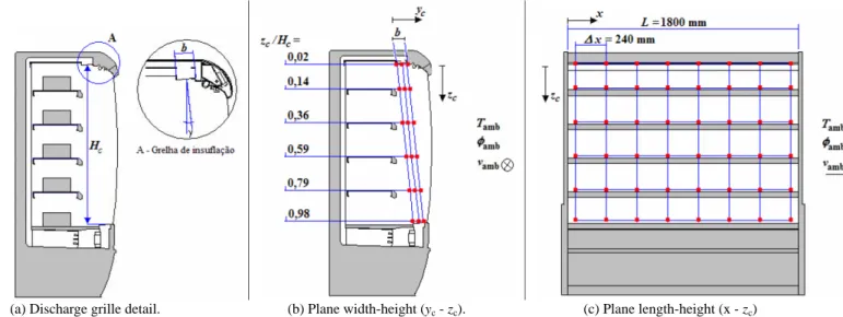
not only dependent of the discharge air velocity as Axell & Fahlén [10] show in their study. Geometric factors like the width of the discharge grille, b, the height of the frontal opening, Hc, and the air curtain angle at the inlet, , (see Fig. 1-a) are also influent on the efficiency, as well as the plug flow through the perforated back panel.
(a) Discharge grille detail. (b) Plane width-height (yc - zc). (c) Plane length-height (x - zc)
Figure 1. Geometric configuration of the display cabinet and experimental probes location.
CFD MODELLING
The display cabinet model used in this study is obtained from a mid cross section (two-dimensional) of the model developed in Gaspar et al. [11] (see Fig. 2). Since Gaspar et al. [11] made experimental measurements of the air velocity, temperature and relative humidity (measurement locations shown in Fig. 1-b and 1-c represented by red dots) based on this ORDC, the results of the simulation can be compared to their experimental results.
The simulations were performed on a 2.2 GHz processor with 2 GBytes RAM on a 32 Bit-system. The used CFD code was Fluent 6.3.26, while the grid was built with Gambit. The grid has a size of 112,836 nodes and 110,029 cells.
Equations
To evaluate the conditions of the system, continuity, momentum, energy and species equations must be solved. Patankar [12] simplified these equations (Eq. 1) for a dependent variable : S x v xk k (1)
For = 1 it is obtained the continuity equation, with = vi the momentum equations, = T the energy equation and for
= ci the species equation. is the diffusion coefficient and S
stands for a general source term. The air is considered as an ideal gas, whose state equation relates the parameters of the substance at equilibrium gas phase state accurately. The buoyancy-driven forces are treated as a source term in the momentum equations.
The energy equation is developed as a function of temperature in a steady state regime with constant specific heat. Further simplifications are accomplished despising viscous dissipation due to the flow characteristics. For modeling the turbulence, the RNG k- model have been taken, which is detailed presented by Yakhot & Orszag [13]. This leads to two more equations, one for the turbulent dissipation and the other for the turbulent kinetic energy. Although the RNG k- model is not assumed to be perfectly accurate [7], it’s a good method to simulate turbulence, when the computational capacity is limited. The influence of ambient relative humidity is considered, making use of a species transport model. The fluid is considered as a mixture of dry air and water vapor. The heat gain of the display case through thermal radiation is considered using a surface-to-surface (S2S) radiation model based in the surfaces view factor calculation [14]. Since the S2S method models the enclosure radiative transfer without participating media, assuming that all surfaces are diffuse and gray radiation, the computation time can be kept low, at some error penalty, after the CPU-intensive view factor calculation.
Numerical model
Since the equations above can’t be solved analytically, they have been discretized and afterwards iteratively solved by several algorithms. The PISO (Pressure-Implicit with Splitting of Operators) algorithm proposed by Issa [15] was considered for the pressure-velocity coupling. The third order MUSCL (Monotone Upstream-Centered Schemes for Conservation Laws) scheme of Van Leer [16] was used to discretize the equations. Solely the turbulent equations were discretized by the first order upwind (FOU) method, as described by Patankar [12]. Each simulation reaches the convergence criterion ( 110-6 for the residuals of the energy equations and 110-3 for the other residuals) at the latest after 4000 iterations. To obtain an optimal comparison between the different simulations, they have been stopped at 4000 iterations. The under-relaxation factors , which reduce the variation of the variables during each iteration, are set as showed in Table 1.
Table 1. Linear relaxation factors.
Property Variable
Pressure p 0.3
Density 0.5
Body forces F 0.5
Momentum vi 0.8
Turbulent kinetic energy k 0.6
Turbulent kinetic energy dissipation rate 0.6
Turbulent viscosity t 0.8
Energy E 0.7
Boundary conditions
The results of this work can be compared with those of Gaspar et al. [11], as most of the boundary conditions (BC) have been assumed to be the same. The BC imposed on the computational domain are those of common practice in numerical simulations, being them defined for the climatic class
n.º 3 of EN-ISO Standard 23953 [17] (Tamb = 25 ºC,
amb = 60 %). However, there are differences at the inlet and at the outlet boundary conditions. As this study considers a two-dimensional model, there is no “room inlet” and no “room outlet”, which provides the ambient air velocity parallel to the equipment's frontal opening.
- Ambient boundary condition
The ambient boundary is simulated by an ‘opening’ type BC, i.e., a constant pressure boundary which allows both inflow and outflow. The pressure value is considered to be the total pressure based on the normal component of the velocity when the flow direction is entering the domain and the static pressure when it is leaving the domain. The ambient temperature is supposed to be Tamb = 25 ºC and the water vapor mass fraction for amb =60 %, is Yv, amb = 11,80 gv/kgm. The radiative black body temperature is assumed to be Tbb = 8.17 ºC, based on the algebraic calculation of the radiative view factors of the enclosure surfaces. This algorithm uses the values from the experimental testing and of typical temperatures, alignment and distances between the surfaces in the corridor where this type of equipments are installed at the supermarkets. For this BC an emissivity is assumed as, = 1. At this fixed-pressure condition employed at free boundary, the free stream values for turbulent kinetic energy and its dissipation rate are assumed in terms of the turbulence intensity, It = 10 %, (the worst situation considering the effects of the passage of the consumer in front of equipment, of the air conditioning system and the influence of pressure perturbations) and the hydraulic diameter of the equipment’s opening to ambient, Dh = 1.2 m, as being the characteristic turbulence length scale.
- Wall boundary condition
Wall BC are used to bound fluid and solid regions. At the walls a shear BC (zero velocity) is considered for non-slip. For the surfaces of the plastic sheet (polipropylene) that enclosure the food products is imposed a thin-wall BC to solve the heat conduction equation computing the thermal resistance offered by the plastic. The values are: = 912 kg m-3; specific heat:
Cp = 1.94 kJ kg-1 K-1; thermal conductivity: k = 0.25 W m-1 K-1; emissivity: = 0.9; and the thickness: = 25.410-6 m.
- Heat flux boundary conditions
For the walls not considered in the heat transfer calculation an adiabatic BC is defined. However, the heat flux BC is used to simulate the heat generated by the illumination (85% for fluorescent lamp OSRAM L58W/20, q = 10 W milum -2) and the heat flux through conduction across the material layers that compose the walls of the equipment. The heat flux across the walls of the equipment is determined by the Fourier Law applying a global heat transfer coefficient determined by conductive thermal resistances of each material of the wall. The experimental temperature values of the interior and exterior surfaces of the equipment are used, varying the values of the
heat flux across the interior surfaces, qintsuf, of the equipment
from 6.1 W m-2 to 7.3 W m-2.
- Species and radiation boundary conditions
A zero-gradient condition for the water vapor mass fraction is assumed at the walls. Since it is considered a surface-to-surface radiation model, it is necessary to specify the emissitivies of the different surfaces. For the internal surfaces of the equipment it is specified a constant emissivity, sup = 0.9 and for the external ground, ground = 0.7. As exposed, for the surfaces of the external enclosure it is considered the black body emissivity, bb = 1.
- Product load (solid region)
Based on the EN-ISO Standard 23953 [17], the products simulators are made of tylose, which thermal characteristics are similar to meat. Its equivalent solid thermal characteristics are imposed considering the values given by ASHRAE [18].
- Fan boundary condition
For the fan (infinitely thin face) is specified a discontinuous pressure rise across it as function of air velocity. The empirical characteristic curve which governs the relationship between head (pressure rise) and flow rate (velocity) across a fan element (obtained at the manufacturer - EBM Papst series 4500) is converted in a 4th order polynomial relationship specified as BC. To achieve different velocities, the polynomial function of the velocity to compute the pressure rise over the fan (Eq. 2) modeled in each setup model is shown in Table 2. The setup n.º 5 is the original setup of the fan in the experiments of Gaspar et al. [11] study.
N n n nv
f
p
1 1 (2)Table 2. Polynomial function of the fan.
Setup n.º vDAG [ms
-1] Polynomial function for p [Pa]
1 0.49 2 3 4 5 8 10 28 20 v v v v 2 0.94 2 3 4 3 12 32 40 v v v v 3 1.15 2 3 4 2 15 40 50 v v v v 4 1.34 2 3 4 2 15 40 55 v v v v 5 1.51 2 3 4 61 . 1 67 . 2 7 . 22 1 . 51 2 . 79 v v v v 6 1.76 2 3 4 5 . 3 38 95 130 v v v v 7 2.40 20090v20v20.5v30.25v4 - Air pressure drop boundary condition at the grilles and perforated back panel (as a porous medium)
The grilles and the perforated back panel are modeled as porous media. The porous medium is modeled by the addition of a momentum source term to the standard fluid flow equations corresponding to the Forchheimer law [19]. The source term is composed of two parts: a viscous loss term
(Darcy, the first term on the right-hand side of Eq. 3), and an inertial loss term (the second term on the right-hand side of Eq. 3) due to high flow velocities [19] and low thickness to hole diameter ratio [20]: i i i i v C v v k S 2 1 2 (3)
Where vi is the average value of fluid velocity through the surface normal to the flow and k is the medium permeability. C2 is the inertial resistance factor. As exposed by Tang et al. [21], the permeability of perforated surfaces can be considered as exposed by Bear [19], in which the thickness of the porous medium, , has an analogical correspondence to the perforation diameter, Dhole: 12 2 k (4)
Where is the porosity (void fraction), i.e., the volume fraction of fluid within the porous region (i.e., the open volume fraction of the medium) given by the ratio between the open volume and total volume of the porous medium.
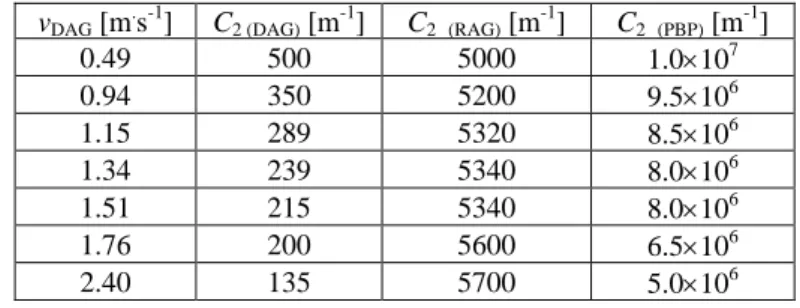
The constant C2 provides a correction for inertial losses in the porous medium. This constant can be viewed as a loss coefficient per unit length along the flow direction. Since the inertial resistance coefficients, C2, of the porous media at the discharge air grille (DAG), at the return air grille (RAG) as well as at the perforated back panel (PBP) vary with changing velocity, all these coefficients were calculated (see Table 3).
Table 3. Inertial resistance coefficients at various velocities.
vDAG [m.s-1] C2 (DAG) [m-1] C2 (RAG) [m-1] C2 (PBP) [m-1]
0.49 500 5000 1.0107 0.94 350 5200 9.5106 1.15 289 5320 8.5106 1.34 239 5340 8.0106 1.51 215 5340 8.0106 1.76 200 5600 6.5106 2.40 135 5700 5.0106
The expressions developed by Idel’Cik [22] are used to calculate the values of the inertial resistance coefficients at the DAG and the RAG which matched quite well with the experimental data. The inertial resistance coefficient for the PBP was calculated making use of an alternative formula presented by Perry & Green [20] for very low Reynolds number. For the original setup, a simulation with
C2 = 8.0106 m-1 provided the same mass flow rate through the PBP like in the experiments of Gaspar et al. [11]. For the other configurations, the velocity through the PBP has to be computed out of the mass flow. The new inertial resistance coefficient, C2, was obtained from the velocity with the relation presented in Eq. 5.
v
C21 (5)
According to [20], this expression is applicable for low Reynolds number (Re 100). This iterative process was performed three times for each setup.
The pressure loss over the evaporator alters as well, but as the influence of this change is negligible, the original value was kept for all setups. A simulation with the DAG velocity of 0.94 ms-1 showed a difference in the velocity of only 0.01 ms-1 between the original pressure loss coefficient (8.33 m-1) and the modified one (12.70 m-1).
As presented by [23,24] and verified by the experimental and numerical results in [11], the higher air temperature is predicted in the conservation zone height extremities, i.e., well tray and top shelf. Based on these results, an additional parametric study is developed which intends to predict the effects of density perforation of the back panel, uniformly and non-uniformly distributed, on the distribution of the air temperature field. The original setup (n.º 5) presents a uniform perforation with Dhole = 4.25 mm (see Table 4). The modified case studies present a double hole diameter, Dhole = 8.50 mm uniformly distributed (n.º 8) and a non uniformly perforation (n.º 9). For this last one, 2/5 of the lower height of the PBP is considered Dhole = 8.5 mm and the original hole diameter in the remainder height (n.º 9). Setup model n.º 10 represents the shifted case. Likewise the previous parametric study, these modifications require the reformulation of the values specified at the BC. These parameters are related to the porous medium formulation used to simulate the PBP. The values of porosity, , viscous, k-1, and inertial, C2, resistance coefficients are presented in Table 4.
Table 4. Parameters specified at PBP boundary condition.
Parameter PBP height, z [%] Setup n.º Variable Unit [0 40] [40 60] [60 100] Dhole mm 4.25 % 2.60 k-1 m-2 2.56107 5 C2 m-1 8.00106 Dhole mm 8.50 % 10.45 k-1 m-2 1.59106 8 C2 m-1 8.42106 Dhole mm 8.50 4.25 % 10.84 2.55 k-1 m-2 1.53106 2.61107 9 C2 m-1 7.23106 2.74109 Dhole mm 4.25 8.50 % 2.65 10.14 k-1 m-2 2.51107 1.64106 10 C2 m-1 2.35109 9.54106
RESULTS AND DISCUSSION
To evaluate the efficiency of the air curtain at the different velocities, the temperatures inside of the ORDC were compared. Lower temperatures mean higher efficiency.
Results
Table 5 shows an overview of the average air temperatures in the whole interior part, at the DAG and at the RAG.
Table 5. Air temperatures in different regions of the ORDC.
vDAG [ms-1] Tcons [ºC] TDAG [ºC] TRAG [ºC]
0.49 5.45 1.63 8.47 0.94 3.57 1.65 4.85 1.15 2.76 1.60 4.95 1.34 3.16 2.05 5.84 1.51 3.67 2.48 6.78 1.76 3.92 3.00 7.51 2.40 4.12 3.59 7.61
The characteristic curve of the air temperature variation in the conservation area for different velocities at the DAG is shown in Fig. 3. The minimum temperature value can be found at a DAG velocity of about 1.15 ms-1, where the air temperature is 2.76 ºC. On the left side of the curve presented in Fig. 3 it can be seen that the temperature increases rapidly, as discharge air velocity decreases. This means that the air curtain is unstable and the warm air through it to the conservation space. On the right side of the curve, with the increasing discharge air velocity, turbulence is generated that stimulates the heat transfer. For this reason the air temperature in the interior rises too. These results allow determining the optimum velocity at the DAG.
2.00 2.50 3.00 3.50 4.00 4.50 5.00 5.50 - 0.50 1.00 1.50 2.00 2.50 3.00 vDAG [ms -1 ] Tco ns [ºC]
Figure 3. Characteristic of the average air temperatures in the interior for various DAG velocities.
The perishable meat products (see Fig. 1) displayed on the equipment's shelves were modeled. The products internal temperature predictions shown in Table 6 were computed in the centre of mass of the “meat” simulator. Product n.º 4 is located on the top shelf of the ORDC, while product n.º 0 is located on the well tray.
Table 6. Internal product temperatures at different heights.
Internal temperatures in the products [ºC]
vDAG
[ms-1] Prod. 4 Prod. 3 Prod. 2 Prod. 1 Prod. 0
0.49 3.50 4.33 3.06 2.48 2.77 0.94 2.58 2.81 2.27 2.36 2.70 1.15 2.57 2.76 2.29 2.44 2.85 1.34 2.64 2.92 2.46 2.64 3.17 1.51 2.76 3.13 2.66 2.89 3.59 1.76 2.87 3.31 2.85 3.15 2.99 2.40 3.00 3.37 3.14 3.64 4.42
The comparison between the products internal temperatures located on the several shelves (Fig. 4) indicates that for low DAG velocities the upper height of the interior part is warmer than the lower one. In these cases the re-circulated air curtain on the front of the higher height shelves is broken (see Fig. 5). The reverse case is predicted at high DAG velocity, as the lower height is much warmer than the upper height. Here, the re-circulated air curtain has no weak zone over the whole height (Fig. 5). The lower height is warmer because the residence time of the air for the heat exchange is greater, the lower the air goes from the DAG to the RAG. In the region of the ideal DAG velocity of 1.15 ms-1, the difference between the air and products temperatures on the five shelves is smaller. Also with this DAG velocity the lowest average air and product temperatures are predicted and determined.
2.00 2.50 3.00 3.50 4.00 4.50 5.00 5.50 - 0.50 1.00 1.50 2.00 2.50 3.00 vDAG [ms -1 ] Tprod [ºC]
Figure 4. Temperature in the five products: Well tray (), Shelve 1 (), Shelve 2 (), Shelve 3 (), Shelve 4 ().
Air velocity field predictions
The experimental tests and 3D CFD modeling performed by Gaspar et al. [11] on this type of ORDC, predicted its higher thermal performance for a DAG velocity of 1.55 ms-1, what means about 0.4 m s-1 higher (i.e. 37 % greater) than in this simulation. Such a deviation was as well detected by Foster et
al. [9], where the optimum velocity founded also is lower in the
simulation, comparing to the experimental data. An explanation for this phenomenon can be the fact that in a 2D simulation,
there is no air movement parallel to the third dimension. Even low velocities of 0.2 ms-1 as defined by the test standard [17] can have quite an influence on the efficiency, like Gaspar et al. [11] have observed in their work. So, the external air movement is assumed to destabilize the air curtain. If the air curtain now runs on low DAG velocities, it is more adaptable than on higher velocities. The re-circulated air curtain at the optimum velocity (1.15 ms-1) is not very robust, as present in Fig. 5-c. By the shelf n.º 2, in the middle of the air curtain, can be seen a zone, where the air curtain is not closed over the whole width anymore. With this weak zone, the air curtain will lose stability very easily after a disturbance from outside (client or air movement) and warm air infiltrates through it to the interior. Therefore a DAG velocity of 1.15 ms-1 would be to low to run the air curtain in real environment. The value of 1.51 ms-1 would be a more appropriate DAG velocity to make sure that the stability of the air curtain is guaranteed. At this velocity, no weak zone in the air curtain appears (Fig. 5-b). Comparing to the Fig. 5-a, which shows the air curtain at a high velocity (2.40 ms-1), no big difference in the quality of the curtain is obvious. The last profile (Fig. 5-d) illustrates the arrangement at the lowest DAG velocity, which was tested (0.49 ms-1). For this situation the numerical predictions profile indicates that the re-circulated air curtain is very weak with breaking regions, being unable to restrict the thermal entrainment from the ambient air, mainly on the top region.
Air temperature field predictions
Considering the numerical predictions profiles of the air temperature, the difference between the efficiency at different DAG velocities is easier to be analyzed (Fig. 6). For a DAG velocity between 1.51 ms-1 (Fig. 6-b) and 2.40 ms-1 (Fig. 6-a), the border between the warm and the cold air is more or less a straight line. In the optimal setup, shown in Fig. 6-c, two regions can be seen where the warm air comes quite close to the interior part. An additional destabilization of the curtain would result on the warm air entrainment. Such an entrainment can be viewed in the last profile (Fig. 6-d), where the warm air nearly reach the second highest shelf. The whole top region of the interior part of the conservation space will be heated up in this situation.
Mass and heat transfer rates
The regions that virtually limits the air curtain (yc/b = 0 and
yc/b = 1) are divided into 5 control volumes to evaluate the mass and heat transfer rates across the air curtain as shown in Fig. 7. For each control volume are determined the mass flow rate and the heat transfer rate for a unit length using Eq. 6 and Eq. 7. A v m [kgs-1] (6) T C m Q p [W] (7)
(a) Setup n.º 7: vDAG = 2.40 ms-1 (b) Setup n.º 5: vDAG = 1.51 ms-1 (c) Setup n.º 3: vDAG = 1.15 ms-1 (d) Setup n.º 1: vDAG = 0.49 ms-1
Figure 5. Air velocity predictions [m s-1] at different DAG velocities.
(a) Setup n.º 7: vDAG = 2.40 ms-1 (b) Setup n.º 5: vDAG = 1.51 ms-1 (c) Setup n.º 3: vDAG = 1.15 ms-1 (d) Setup n.º 1: vDAG = 0.49 ms-1
Figure 6. Air temperature predictions [°C] at different DAG velocities.
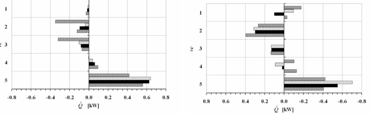
The values and directions of the heat transfer across the air curtain for a unit length are shown in Fig. 8 for the fan velocity-pressure rise setup models n.º 1, n.º 3, n.º 5 (original setup) and n.º 7. These predictions indicate that for all setup models the air curtain gains thermal energy from the external ambient and from the conservation region. These gains are related to the ambient air infiltration, thermal radiation, illumination and heat conduction through the equipment's walls.
The mass flow rate across the inner border promotes the mixture between the refrigerated air discharged by the air curtain and the conservation air. When followed by an increase of the mass flow rate that crosses the outer border, there is a higher thermal entrainment reducing the air curtain efficiency.
It must be taken into account the influence of the plug flow from the PBP.
The setup model n.º 7 predicts an air discharge velocity greater than the original setup (n.º 5), vDAG = 2.40 ms-1. Globally, in this case are predicted the highest mass flow rates both in and out of the faces of the inner border of the air curtain. This high fan velocity also provides a higher mass flow rate through the PBP. The setup model n.º 1 predicts the lowest air discharge velocity. The air curtain is break up as it travels from the DAG to the RAG due to its low momentum. In this case are predicted the highest mass flow rates both in and out of the faces of the outer border of the air curtain. This condition provides the highest heat transfer out of the inner faces of the air curtain to the products conservation zone. The setup models
n.º 3 and n.º 5 present a proper aerothermodynamics barrier since the air temperature in the conservation space is below 3.00 ºC. The comparison of the numerical predictions of the different model setups indicates that the fan models setup n.º 3 and n.º 5 can improve the global performance of the display cabinet.
The increase of the holes diameter will increase the mass flow rate by the PBP and reduces the mass flow rate through the DAG. In Fig. 9 are presented the values and directions of the mass flow rates across the air curtain for a unit length for the setup models with different hole diameter and distribution of the PBP. The comparative analysis of the numerical predictions from [11] indicates that the vortex formation in the upper shelf is suppressed by the reduction of the DAG velocity. These modifications increase the mass flow and heat transfer rates through the outer border of the air curtain and decrease them in the inner border, being the differences not so pronounced.
Figure 7. Air curtain region subdivision into 2D volumes of control.
a) West faces, w (Inner border). b) East faces, e (Outer border).
Figure 8. Heat transfer rate predictions across West (inner border) and East (outer border) of the control volumes of the air curtain, for a unit length – fan modification case study. Legend: Setup n.º 1 ( );Setup n.º 3 ( ); Setup n.º 5 ( ); Setup n.º 7 ( ).
a) West faces, w (Inner border). b) East faces, e (Outer border).
Figure 9. Mass flow rate predictions across West (inner border) and East (outer border) of the control volumes of the air curtain, for a unit length – back panel perforation modification case study. Legend: Setup n.º 5 ( );Setup n.º 8 ( );Setup n.º 9 ( );Setup n.º 10 ( ).
The numerical predictions indicates that a slight DAG velocity reduction reduces the thermal entrainment at higher heights of the air curtain (near the DAG) but increases it at the lower heights (near the RAG) due to air curtain momentum reduction. This situation is verified by the analysis of the mass flow rate at the lowest control volume (vc 5).
These modifications allow the reduction of the air temperature near the PBP. Additionally, allow a lower air temperature returned to the evaporator. Comparing the thermal and temperature ratios relatively to original setup n.º 5, all of the new setups (n.º 8 to n.º 10) predict a reduction of the total heat transfer rate across the air curtain ranging between 21 % to 23 %. Although, only setup n.º 8, where it is considered an uniformly distributed doubled hole diameter, predicts a 4 % reduction of the air temperature in the conservation zone relatively to the setup n.º 5. The increase of mass flow rate through de PBP allows the reduction of the air discharge (8 %) and return (9 %) temperatures. Based on these numerical results, is suitable to double the perforation diameter with uniform distribution due to the predicted reduction of the thermal load and lower air temperature.
CONCLUSION
A CFD modeling of an open refrigerated display cabinet is developed considering low cost geometrical and operational characteristics modifications to predict an improvement of the global performance and energy efficiency. The parametric studies are devoted to the analysis of the thermal behavior influenced by the fans velocity, and by the density and distribution of the back panel’s perforation.
The parametric study results as the fan velocity varies predicts that the optimum DAG velocity of 1.15 ms-1 is lower than expected. Since the re-circulated air curtain has a weak zone, additional experiments have to prove the stability of the air curtain for a DAG velocity of 1.15 ms-1. If after an interference from outside, like will be normal and possible in a supermarket, the warm air infiltrates into the conservation space of the ORDC, so the DAG velocity should be increased to the value of 1.51 ms-1. The influence of the ambient air flow velocity to the air curtain stability must be clarified in future work, since the optimum DAG velocity should vary depending on the ambient air flow. If this is the case, the DAG velocity can be reduced in a supermarket, when the disturbance is lower and increased, when the ambient air flow is higher.
The parametric study results as the holes density and distribution of the back panel perforation is modified, reveals the significance of the binomial between the DAG and PBP mass flow rates. A minimum DAG velocity is required to provide a sufficient air momentum able to keep a stable aerothermodynamics barrier between the DAG and the RAG. However, a minimum PBP velocity is also required to maintain an unbroken air curtain away from the shelves. If these velocities are higher than the specified values, one of two conditions can occur. A high DAG velocity will promote the air mixture on both the inner and outer border of the air curtain, thus increasing the thermal entrainment. For the same fan, a
higher back panel perforation will increase the air velocity through the holes and consequently reduce the DAG velocity as well as the strength of the air curtain. Moreover, the higher momentum of this plug flow will push the air curtain away from the RAG, increasing the return air temperature and the energy consumption of the equipment.
The results obtained allow improving the food safety and increasing the conservation time period in cold. Moreover, the CFD model developed allows testing in the future relevant factors that may affect the display cabinet global performance, such as, evaporator dimensions and its heat transfer rate, grilles grid, shelves width, among others.
These numerical predictions considering geometrical and operational modifications applied to the open refrigerated display cabinets can be used as a design tool, revealing the capabilities of CFD in an initial project phase, allowing testing several configurations with reduced cost and time. These numerical results can be used as design constrains of the project in order to obtain a final product with an improvement of the energy consumption rationalization facing the increasing exigencies both from sector’s regulation concerning quality and food safety.
NOMENCLATURE General
2D Two-dimensional.
A Area, [m2].
b Air curtain width, [m].
BC Boundary condition.
C2 Pressure-jump (inertial resistance) coefficient, [m-1].
ci Concentration of species i.
Cp Specific heat, [J kg-1 K-1]. DAG Discharge air grille.
Dh Hydraulic diameter, [m].
H Height, [m].
It Turbulence intensity, [%].
k Turbulent kinetic energy, [m2 s-2]; Permeability, [m2].
L Length, [m].
m Mass flow rate, [kg s-1]
p Pressure, [Pa]. PBP Perforated back panel.
q Heat flux, [W m-2].
Q Heat transfer rate, [W].
Re Reynolds Number.
S General source term.
T Temperature, [ºC].
v Average velocity, [m s-1].
W Width, [m].
Y Mass fraction, [kgv/kgm]. RAG Return air grille.
vc Control volume.
x , y , z Spatial coordinates, [m].
yc, zc Discharge grille reference frame, [m].
Superscripts and subscripts
avg Average. bb Black body.
c Air curtain.
cons Conservation. DAG Discharge air grille. evap Evaporator.
e, w Control volume faces (East, West). m Mixture.
RAG Return air grille. v vapor.
Greek Symbols
Linear relaxation factor.
Density, [kg m-3].
Dissipation rate of k, [m2 s-3]; Emissivity; Porosity.
Relative humidity, [%]; General variable.
Dynamic viscosity, [kg m-1 s-1].
Diffusion coefficient.
Curtain angle at the discharge, [ º ]. Convergence criterion. p Pressure loss/rise [Pa]. T Temperature difference [ºC]. ACKNOWLEDGMENTS
The authors wish to acknowledge the support of University of Beira Interior – Engineering Faculty – Electromechanical Engineering Department and of the refrigerated display cabinet manufacturer JORDÃO Cooling Systems®, Guimarães, Portugal (www.jordao.com).
REFERENCES
[1] Faramarzi, R., 1999, "Efficient display case refrigeration," ASHRAE Journal 41(11).
[2] Cortella, G., Manzan, M. and Comini, G., 2001, "CFD simulation of refrigerated display cabinets," Int. J. Refrigeration 24(3), 250-260.
[3] Ge, Y.T., Tassou, S.A., 2001, "Simulation of the performance of a single jet air curtains for vertical refrigerated display cabinets," Int. J. Refrigeration 21(2), 201–209.
[4] Navaz, H.K., Henderson, B.S., Faramarzi, R., Pourmovahed, A., Taugwalder, F., 2005, "Jet entrainment rate in air curtain of open refrigerated display cases," Int. J. Refrigeration 28(2), 267-275.
[5] Chen, Y.-G., Yuan, X.-L., 2005, "Simulation of a cavity insulated by a vertical single band cold air curtain," Energy, Conversion & Management 46(11-12), 1745-1756.
[6] D’Agaro, P, Cortella, G., Croce, G., 2006, "Two- and three-dimensional CFD applied to vertical display cabinets refrigeration," Int. J. Refrigeration 29(2), 178-190.
[7] Smale, N.J., Moureh, J., Cortella, G., 2006, "A review of numerical models of airflow in refrigerated food applications," Int. J. Refrigeration 29(6), 911-930.
[8] Norton, T, Sun, D.-W., 2006, "CFD-an effective and efficient design and analysis tool for the food industry: a
review," Trends in Food Science & Technology. 17(11), 600-620.
[9] Foster, A.M., Swain M.J., Barrett, R., et al, 2006, "Effectiveness and optimum jet velocity for a plane jet air curtain used to restrict cold room infiltration," Int. J. Refrigeration 29(5), 692-699.
[10] Axell, M., Fahlén, P., 2003, "Design criteria for energy efficient vertical air curtains in display cabinets," Proc. of 21st IIR Int. Congress of Refrigeration, Washington DC, U.S.A. [11] Gaspar, P.D., Gonçalves, L.C.C, Pitarma, R.A., 2008, "Three-dimensional CFD modelling and analysis of the thermal entrainment in the open refrigerated display cabinets," Proc. of the 2008 ASME Summer Heat Transfer Conference, Jacksonville, U.S.A.
[12] Patankar, S.V., 1980, "Numerical Heat Transfer and Fluid Flow," Hemisphere Publishing Corporation.
[13] Yakhot, V., Orszag, S.A., 1986, "Renormalization Group Analysis of Turbulence: I. Basic Theory," J. of Scientific Computing 1(1).
[14] Modest, M.F., 1993, "Radiative heat transfer," McGraw-Hill, Inc.
[15] Issa, R.I., 1985, "Solution of the implicitly discretized fluid flow equations by operator-splitting," J. Computational Physics 62.
[16] Van Leer, B., 1979, "Toward the ultimate conservative difference scheme, IV, a second order sequel to Godunov's method," J. of Computational Physics 32.
[17] EN-ISO Standard 23953. 2005, "Refrigerated display cabinets, parts 1 and 2," ISO - International Organization for Standardization.
[18] ASHRAE, 1997, "ASHRAE Handbook: Fundamentals," American Society of Heating, Refrigerating and Air-Conditioning Engineers Inc.
[19] Bear J., 1988, "Dynamics of fluids in porous media," Mineola: Dover Publications Inc.
[20] Perry, R.H., Green, D.W., 1999, "Perry’s chemical engineers’ handbook," McGraw Hill, Inc.
[21] Tang, L., Moores, K.A., Ramaswamy, C., Joshi, Y., 1988, "Characterizing the thermal performance of a flow through electronics module (SEM-E Format) using a porous media model," In: Proc. of 14th IEEE SEMI-THERMTM Symposium, IEEE.
[22] Idel’Cik, I.E., 1969, "Memento de pertes de charges," Direction des Études et Recherches D’électricité de France. [23] Chen, Y.-G., Yuan, X.-L., 2005, "Experimental study of the performance of single-band air curtains for multi-deck refrigerated display cabinet," J. Food Engineering 69(3), 261-7. [14] Gray, I. et al., 2008, "Improvement of air distribution in refrigerated vertical open front remote supermarket display cases," Int. J. Refrigeration 31(5), 902-10.


![Figure 6. Air temperature predictions [°C] at different DAG velocities.](https://thumb-eu.123doks.com/thumbv2/123dok_br/18153306.872191/7.892.78.846.482.784/figure-air-temperature-predictions-at-different-dag-velocities.webp)