1. INTRODUCTION
Traffic congestion cost reached US$ 115 billion in urban areas in the USA in 2009 (Schrank et al., 2010), while in Europe the traffic congestion cost was estimated at € 100 billion in 2010 (European Comission, 2011). This is not surprising in view of the observed increasing road conges-tion extent around the globe and the fact that transport and mobility are one of the main drivers of the economical and technological development (Isermann, 2011).
Congestion forming on a freeway affects the nominal freeway capacity and throughput giving rise to an escalation of infrastructure degradation as a result of the absence of suitable traffic control measures that would counter and lim-it the congestion evolution. Thus, freeways need to be con-trolled for maximum efficiency, increased safety and re-duced emission of pollutants. Indeed, transportation, in its different modes, is foreseen as one of the most challenging areas where future developments of automatic control are mostly expected (Isermann, 2011; IEEE, 2011).
A recent concept for freeway traffic flow control is Main-1
Rodrigo Castelan Carlson, Center for Mobility Engineering and Post-graduate Program in Automation and Systems Engineering, Federal University of Santa Catarina, Joinville, SC, Brasil. (e-mail: [email protected]) 2
Ioannis Papamichail, Dynamic Systems and Simulation Laboratory, Tech-nical University of Crete, Chania, Greece. (e-mail: [email protected]) 3
Markos Papageorgiou, Dynamic Systems and Simulation Laboratory, Technical University of Crete, Chania, Greece. (e-mail: [email protected])
Manuscrito recebido em 23/09/2013 e aprovado para publicação em 29/10/2013. Este artigo é parte de TRANSPORTES v. 21, n. 3, 2013. ISSN: 2237-1346 (online). DOI:10.4237/transportes.v21i3.694.
stream Traffic Flow Control (MTFC) as introduced by Carl-son et al. (2010a, 2010b) using a nonlinear optimal control method. MTFC aims at directly influencing the freeway mainstream flow via an appropriate actuator, such as varia-ble speed limits (VSLs), and may complement existing traf-fic control measures.
MTFC-like concepts had been investigated already in the 1960s (Greenberg e Daou, 1960; Gazis e Foote, 1969). With the increased interest in VSL systems, mainstream flow control strategies based on the use of VSLs were pro-posed and investigated for a variety of traffic application settings and control approaches, including optimal control (Alessandri et al., 1998), robust control (Chiang e Juang, 2008), feedback control (Zhang et al., 2006), model-predictive control (Hegyi et al., 2005), distributed control (Popov et al., 2008), and rule-based control (Lin et al., 2004). Most of these VSL-based strategies, however, are not deemed sufficiently mature for a practical application, see Carlson et al. (2011a). A noteworthy exception seems to be the recent SPECIALIST effort (Hegyi e Hoogendoorn, 2010) which demonstrated that mainstream traffic flow reg-ulation via VSLs actually works in practice, albeit based on a feed-forward approach. The reader is referred to Carlson et al. (2011a) for more details on past work.
In an attempt to circumvent the practical limitations of some of the previous methods, Carlson et al. (2011a) pro-posed, based on the same MTFC application concept of Carlson et al. (2010a, 2010b), a simple, yet efficient VSL-based MTFC feedback cascade controller that is deemed suitable for ready field implementation. This paper demon-strates the use of the two controllers developed by Carlson
freeways using variable speed limits
Rodrigo Castelan Carlson1, Ioannis Papamichail2 e Markos Papageorgiou3
Abstract: Mainstream Traffic Flow Control (MTFC), enabled via variable speed limits, is a control concept for real-time freeway
traf-fic management. The benefits of MTFC for eftraf-ficient freeway traftraf-fic flow have been demonstrated recently using an optimal control ap-proach and a feedback control apap-proach. In this paper, both control apap-proaches are reviewed and applied to a freeway network in a simulation environment. The validated network model used reflects an actual freeway (a ring-road), fed with actual (measured) de-mands. The optimal and feedback control results are discussed, compared and demonstrated to improve significantly the system per-formance. In particular, the feedback control scheme is deemed suitable for immediate practical application as it takes into account op-erational requirements and constraints, while its results are shown to be satisfactory. In addition, the control system performance was not very sensitive to variations of the parameters of the feedback controller. This result indicates that the burden associated with fine tuning of the controller may be reduced in the field.
DOI:10.4237/transportes.v21i3.694.
Keywords: freeway traffic control, mainstream traffic flow control, variable speed limits, feedback control, optimal control.
Resumo: Controle do Fluxo Principal (CFP), realizado via limites de velocidade variáveis, é um conceito de controle para o
gerenci-amento em tempo real do tráfego em rodovias. Os benefícios de CFP para a fluidez do tráfego foram demonstrados por pesquisas re-centes que utilizaram uma abordagem de controle ótimo e uma abordagem de controle realimentado. Neste artigo, as duas abordagens de controle são revisadas e aplicadas a uma malha rodoviária em um ambiente de simulação. O modelo utilizado da malha rodoviária, que reproduz um anel viário real, foi validado e alimentado com demandas medidas em campo. Os resultados de controle ótimo e con-trole realimentado são discutidos e comparados, e produzem melhora significativa no desempenho do sistema. A estrutura de concon-trole realimentado é considerada apropriada para a aplicação em campo, uma vez que considera requisitos e restrições operacionais, e apre-senta resultados satisfatórios. Além disso, o desempenho do sistema de controle mostrou pouca sensibilidade a variações nos parâme-tros do controlador realimentado. Este resultado indica que os esforços para sintonia do controlador em campo podem ser reduzidos. Palavras-chave: controle de tráfego rodoviário, controle do fluxo principal, limites de velocidade variáveis, controle realimentado, controle ótimo.
et al. (2010a, 2010b, 2011a) for the MTFC on freeways via VSLs. A new set of simulation experiments of an actual freeway (a ring-road) using actual (measured) demands demonstrates the controllers' main features under realistic conditions – in fact the closest to reality one can reach be-fore field implementation. Furthermore, since fine-tuning of the feedback controller is an unavoidable task in practice, the performance of the closed-loop system is evaluated with respect to variations of the parameters of the controller and is shown to exhibit low sensitivity to these variations.
In the next section, some basic insights related to freeway traffic control are presented, and the MTFC concept is re-viewed; in addition, the essentials of the METANET simu-lator (Messmer e Papageorgiou, 1990; Carlson et al., 2010b) used for the evaluation of the controllers is outlined. Section 3 recapitulates the optimal control strategy imple-mented within the AMOC optimal control tool (Kotsialos et al., 2002b; Carlson et al., 2010b) and the MTFC feedback cascade controller designed by Carlson et al. (2011a). The optimal control and feedback control strategies are com-pared and have their efficiency evaluated in Section 4. Fi-nally, Section 5 concludes the paper and comments on fur-ther research on the subject.
2. BACKGROUND
2.1. The fundamental diagram
The traffic flow states may be approximated by the funda-mental diagram, which is usually represented as a flow q (veh/h) versus density ρ (veh/km) diagram, as in Figure 1(a). The point of maximum flow in the diagram corre-sponds to the capacity flow qcap at the freeway location
where the diagram was obtained, while the corresponding traffic density value is called the critical density ρcr. The
mean speed of a particular traffic state on the flow-density diagram is the slope of the line that connects the particular traffic state point with the origin. A critical (mean) speed vcr
is associated to the state of capacity flow.
2.2. Congestion-caused infrastructure degradation
A bottleneck on a freeway is a location where the flow ca-pacity up
cap
q upstream is higher than the flow capacity down cap
q
downstream of the bottleneck location (Figure 2(a)). If the arriving flow qin is higher than down
cap ,
q the bottleneck is ac-tivated, i.e., congestion is formed. Congestion forming at an active bottleneck has two detrimental effects on freeway ca-pacity and throughput (Papageorgiou e Kotsialos, 2002):
Capacity drop (CD) at the congestion head, i.e., an active bottleneck outflow qout that may be 5-25 % lower than the nominal capacity down
cap ,
q see, e.g., Chung et al. (2007). A main contributing factor for CD occurrence is deemed to be the acceleration of vehicles while exiting the congested area; and Blocking of off-ramps (BOR): vehicles that are
bound for exits upstream of the active bottleneck, are also delayed due to the blocking of the correspond-ing ramps by the congestion body, while the off-ramp flow is reduced.
2.3. The MTFC concept
The basic idea of MTFC is to regulate the mainstream traf-fic flow suftraf-ficiently upstream (some 500 m) of (otherwise) active bottlenecks, so as to avoid the CD (since vehicles will have accelerated before reaching the bottleneck area) and establish maximum bottleneck throughput (Figure2(b)). The bottleneck of Figure 2(b) is not activated (and no MTFC is needed) as long as qin≤qcapdown, in which case
out ≈ in
q q . If qin grows bigger than the bottleneck capacity
down cap
q , the bottleneck would be activated in absence of con-trol as in Figure 2(a), and qout would be reduced due to CD; while MTFC can implement a controlled mainstream flow
c
q , such that qout is equal to qcapdown. Clearly, the main-stream congestion cannot be avoided via MTFC, because
(a) (b)
Figure 1. (a) Flow-density (fundamental) diagram and (b) fundamental diagram for different VSL rates
(a) (b)
congestion outflow in the MTFC case is higher than in the no-control case, because the capacity drop is avoided; hence the controlled congestion is space-time shorter than in the no-control case (and thus the BOR effect is accordingly re-duced). Further details on the benefits of MTFC can be found in Carlson et al. (2010a, 2010b, 2011a).
In this paper, variable speed limits (VSLs) are used as an MTFC actuator to impose the controlled flow qc on the freeway mainstream. The use of VSLs requires considera-tion of several implementaconsidera-tion issues that were detailed by Carlson et al. (2010a, 2011a).
2.4. Traffic flow simulation model (METANET)
A validated macroscopic second-order traffic flow model included in the METANET freeway traffic flow simulator (Messmer e Papageorgiou, 1990) that incorporates VSL control measures (Carlson et al., 2010b) was used in this work.
The freeway network is represented by a directed graph, whereby the links of the graph represent freeway stretches with uniform characteristics. The nodes of the graph are placed at locations where a major change in road geometry occurs, as well as at junctions and on-/off-ramps. The time and space arguments are discretized. The time step is denot-ed by T (typically T =10 s). A freeway link m is divided into Nm segments of equal length Lm (typically Lm =500 m). The traffic in each segment i of link m at discrete time
, =
t kT k=0, 1,, is macroscopically characterized via the following variables: the traffic density ρm i,
( )
k(veh/km/lane) is the number of vehicles in segment i of link m at time t=kT divided by Lm and by the number of lanes λm; the mean speed vm i,
( )
k (km/h) is the mean speedof the vehicles in segment i of link m at time t=kT and ; the traffic volume or flow qm i,
( )
k (veh/h) is the number of vehicles leaving segment i of link m during the time peri-od kT k,(
+1)
T divided by)
T.The density and mean speed are state variables calculated from the conservation equation and a dynamic speed equa-tion, respectively (see Messmer and Papageorgiou (1990)); flows are calculated from
( )
( ) ( )
, =ρ , , λ .
m i m i m i m
q k k v k (1)
The dynamic speed equation includes a static speed-density relationship, which is equivalent to a fundamental diagram, that incorporates the impact of variable speed lim-its. Particular VSL values are reflected in corresponding link-specific VSL rates bm
( )
k that prevail, by definition, during[
kT k, ( +1)T)
, at link m (or a cluster of links). The VSL rate b is approximately equal to the displayed VSL m divided by the legal speed limit without VSL. The VSL rates are control variables with bm( )
k ∈ bmin,m,1.0 wheremin,m
b is a lower admissible bound, while bm =1.0 means no VSL displayed. The kind of changes incurred to the fun-damental diagram via the VSLs may be viewed in Figure 1(b) and are attributed to the reduced speeds at undercritical
of the speed limits (see, e.g., Papageorgiou et al. (2008)). METANET also includes appropriate modeling equa-tions for network nodes, that involve, among others, the dy-namics of origin (e.g., on-ramp) queues wo; for further de-tails, see Messmer and Papageorgiou (1990).
The nonlinear macroscopic traffic flow model outlined above may be formulated as a discrete-time state-space model for the entire freeway network:
(
+ =1)
( ) ( ) ( )
, , ,( )
0 = 0x k f x k u k d k x x (2)
with x the state vector, u the control vector and d the dis-turbance vector. The state vector consists of the densities
,
ρm i and the mean speeds vm i, of every segment i of every link m, and the queues wo of every origin o . The control vector consists of the VSL rates bm of every link m where VSL is applied (otherwise b≡1.0). The disturbance vector consists of the demand do at every origin o and the turning rates βm
n at every bifurcation node n towards out-link .m 2.5. VSLs as an MTFC actuator
The applicability of MTFC via VSLs relies mainly on the utilization of two aspects of the effect of VSLs on the ag-gregate traffic flow behavior (Carlson et al., 2010b, 2011a): If the mainstream demand qin (Figure 2(b)) arriving from upstream is lower than the VSL-induced capac-ity, then the application of VSL will temporarily (for the duration of the traffic state transition triggered by the VSL) decrease the mainstream flow arriving in the bottleneck area; after this transition period, the outflow from the VSL application area returns to values equal to the upstream arriving demand qin
(Figure 1(b)). This temporary flow reduction may be exploited to temporarily hold back traffic flow in or-der to retard the onset of congestion at the down-stream bottleneck; and
Sufficiently low VSL values lead to accordingly lower flow capacity in the fundamental diagram (Figure 1(b)). This implies that, if the mainstream demand qin (Figure 2(b)) arriving from upstream is higher than the VSL-induced capacity, then the VSL application area becomes an active mainstream bot-tleneck that limits the area's outflow qc to values corresponding to the (lower) VSL-induced capacity; this provides the possibility to apply a more durable mainstream flow control, which persists even after the transition period. Thus, a controllable main-stream bottleneck may be created deliberately up-stream of a bottleneck location to avoid its activation and the related reduction of throughput because of the capacity drop.
The above two aspects cannot be associated to a specific VSL range in a freeway, since they depend also on the ar-riving demand qin. Additionally, lower VSL rates shift the critical density of the fundamental diagram towards higher values (Figure 1(b)).
3. OVERVIEW OF MAINSTREAM TRAFFIC FLOW CONTROLLERS
In this section two mainstream traffic flow controllers are reviewed. First, the optimal control approach is reviewed and then the cascade feedback controller.
3.1. Nonlinear constrained optimal control (AMOC software tool)
The freeway network traffic control problem may be formu-lated as a discrete-time nonlinear dynamic optimal control problem with constrained control variables over a given op-timization horizon KP, and is incorporated in the open-loop optimal control tool AMOC (Kotsialos et al., 2002b). The general formulation of the optimal control problem reads:
Given disturbance predictions d k
( )
, k=0, 1,,KP−1,and the initial state x
( )
0 =x0; minimize( )
P 1( ) ( ) ( )
P 0 , , ϑ −ϕ = = x +∑
x u d K k J K k k k (3)subject to (2) and bmin,m ≤bm ≤1.0.
The chosen cost criterion is the total time spent (TTS) by all vehicles in the network, including the waiting time expe-rienced in the ramp queues. Moreover, a low-weighted term may be added to penalize (abrupt) time variations of the op-timal VSL rate trajectories (Carlson et al., 2010b).
The AMOC solution consists of the optimal VSL rate and state variable values within the horizon KP that minimize the TTS. Common VSL rates can be considered for clusters of links.
The optimal control problem delivers ideal solutions in a simulation environment due to the “perfect” model, the ex-act knowledge of (future) disturbances (demands and turn-ing rates) and the lack of some VSL constraints. Clearly, these solutions cannot be outperformed (in simulation) by any other control strategy but may be used to assess the ef-ficiency of other (simpler) strategies under different scenar-ios. In practice, unless the optimal control strategy is cast in a model-predictive framework (Papamichail et al., 2010), the solution from the optimal control approach becomes suboptimal due to various inherent uncertainties.
3.2. Feedback controller
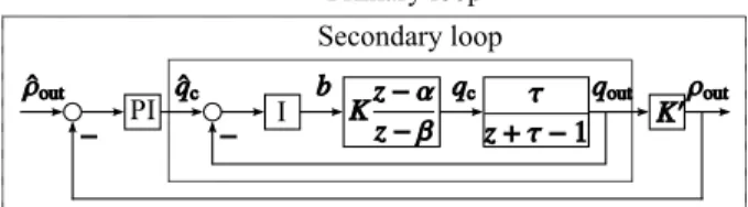
The control problem implied within Figure 2(b) is to regu-late the traffic density ρout (the control output) via appro-priate real-time changes of the mainstream flow q which c, are enabled via the display of appropriate VSLs upstream of the bottleneck location with the VSL rate b as the control input.
The basis for the design of the feedback MTFC via VSLs is a discrete-time linearized model (Carlson et al., 2011a):
( )
( )
out 1 ρ τ α τ β ∆ = ⋅ ′ ⋅ − ∆ + − − z z K K b z z z (4)with α, β, τ, K′ >0 and K >0 being model parame-ters, and 0< < ≤ z the discrete-time complex varia-β α 1; ble; ∆ρout the density variation at the bottleneck location
due to a variation ∆b at the application area.
Figure 3 depicts the MTFC feedback cascade structure designed by Carlson et al. (2011a). The internal loop in Figure 3 is affected by the VSL rate b delivered by the secondary controller that will determine the outflow qc of Figure 2(b). The secondary controller was designed as an integral (I) regulator:
( )
=(
− +1)
I q( )
b k b k K e k (5)
with KI the integral gain and eq
( )
k =q kˆc( )
−q kc( )
the flow control error.The flow qc measured downstream of the application ar-ea is used as a reference for the primary controller and is fed back and compared to the reference flow qˆc delivered by the primary controller. The primary controller uses the measured density ρout at the bottleneck area and compares it with the set-point density ρˆout, which is set equal to the critical density ρcr for throughput maximization. The pri-mary controller was specified to be a proportional-integral (PI) regulator:
( )
(
) (
) ( )
(
)
c c P I P
ˆ = ˆ − +1 ′+ ′ ρ − ′ ρ −1
q k q k K K e k K e k (6)
with KI′ e KP′ the integral and proportional gains of the controller, respectively, and eρ
( )
k =ρˆout−ρout( )
k the den-sity error. For more details about the controller design, tun-ing and operation, see Carlson et al. (2011a).3.2.1. VSL application aspects
This section summarizes some practical VSL implementa-tion aspects detailed in Carlson et al. (2011a). To start with, VSLs can only take discrete values in practice. Therefore, a set of admissible discrete VSL rates b∈
{
0.1, 0.2,, 1.0}
is defined and the discrete VSL rate to be applied is obtained by rounding off the VSL rate b k( )
delivered by the control strategy (5). As further constraints, the difference between two consecutive posted VSL rates at the same variable mes-sage sign (VMS) is limited to 0.2. Similarly, the difference between the posted VSL rates at two consecutive VMSs is also limited to 0.2. Furthermore, a constant VSL rate of 0.9 is applied in the acceleration and bottleneck areas whenever the MTFC via VSL system is active. Finally, for traffic safety reasons, additional VSLs may be activated within and upstream of the controlled congestion in a way that vehicles driving towards the congestion tail encounter gradually de-creasing VSLs. These practical aspects are only considered when applying feedback concepts, not with AMOC optimal control results (see Section 3.1).Figure 3. Cascade MTFC feedback structure using VSL as an
ent control scenarios are discussed in this section. First, the network is simulated without any control measure, as a base reference, using the METANET simulator. Next, the net-work is tested under optimal MTFC via VSLs, as an upper limit of achievable performance under ideal conditions, us-ing the AMOC optimal control tool. Then, the freeway is simulated with feedback cascade MTFC via VSLs, with and without the constraints described in Section 3.2.1, using the METANET simulator. The simulated scenarios and result-ing TTS are summarized in Table 1. Finally, an additional set of simulations with the feedback cascade controller is run to evaluate the sensitivity of system performance with respect to variations in the controller's parameters.
4.1. The Amsterdam ring-road
For this study, the counter-clockwise direction of the Am-sterdam ring-road A10 is considered (Figure 4). This free-way is about 32 km long and has 21 on-ramps, including the freeway-to-freeway junctions with A1, A2, A4 and A8, and 20 off-ramps, including connections with A1, A2, A4 and A8. The merge area of A1 (OA1) with A10 at L107 is the main recurrent active bottleneck of the network. The model parameters were determined from validation of the network traffic flow model against actual data, see Kotsialos et al. (2002a); while the VSL-specific parameters were chosen such that the VSL-induced capacity qcap,m*
( )
bm is not higher than the non-VSL capacity qcap,m for any VSL value (Carl-son et al., 2010a), as sketched in Figure 1(b).The ring-road was studied for a time horizon of 4 h using measured demands from the site. For the controlled scenari-os, the frequency of VSL changes is determined by the
con-(2011a, 2013) for details on the choice of the control peri-od). The simulation time step is T =10 s.
4.2. No-control case
When simulating the network without any control measures, heavy congestion appears in the freeway and large queues are built in some on-ramps. The related density and queue profiles are displayed in Figure 5(a-b). Congestion is formed shortly after the beginning of the simulation (Figure 5(a)) as a consequence of the excessive demand and the ab-sence of control measures. This traffic jam originates at the junction of A1 with A10 and propagates upstream, blocking A4 and a large part of the A10-West. The density at the bot-tleneck area (merge area of A1; first segment of L107) is shown by the black curve in Figure 6(a) and is clearly over-critical (the over-critical density is ρ =cr 32 veh/km/lane) for most of the simulation duration. The corresponding flow at the bottleneck area of around 5400 veh/h is shown in Figure 6(b), and is below capacity (qcap,L107 =5900 veh/h) because of a capacity drop of around eight percent.
After the first traffic jam is partially dissolved, a new one appears leading to more severe congestion. This strong congestion keeps the A4 entrance to the A10 blocked, which results in the queues at the freeway-to-freeway on-ramp of A4 and at the surrounding on-on-ramps (Figure 5(b)). Likewise, off-ramp outflows are affected by the congestion mounting upstream, but further details on this issue are postponed to the subsections that follow. The TTS for this scenario is equal to 14,163 veh·h. The described no-control simulation results are very similar to the corresponding real afternoon-peak traffic conditions (Kotsialos et al., 2002a). Table 1. Summary of Simulated Control Scenarios
Strategy Description TTS (veh·h) %
No-control
The network is simulated without any control measures using the
METANET simulator. 14,163 -
Optimal Control (AMOC)
The network is simulated for optimal MTFC via VSLs using the AMOC
optimal control tool. 8,675 –38.8
Feedback Control (FB)
The network is simulated for feedback MTFC via VSLs using the
METANET simulator without any constraints. 9,315 –34.2 Feedback Control
(with constraints)
The network is simulated for feedback MTFC via VSLs using the METANET simulator with discretized VSL rates, limited VSL rate
variation, and bL105-L107 = 0.9 9,184 –35.2
Feedback Control (with constraints and safety speed limits)
The network is simulated for feedback MTFC via VSLs using the METANET simulator with discretized VSL rates, limited VSL rate
variation, bL105-L107 = 0.9 and safety speed limits. 9,513 –32.8
4.3. Nonlinear optimal control (AMOC)
Next, MTFC via VSLs is applied using nonlinear optimal control (AMOC). In contrast to Carlson et al. (2010a), only one cluster of links, L101-L102, is considered in this inves-tigation, i.e., VSLs are applied locally in the area near the bottleneck location, similarly to what is done with local feedback in the next section.
The resulting TTS value for this scenario is equal to
8,675 veh·h, which is a 38.8 percent improvement com-pared to the no-control case. The related density and ramp queue profiles are shown in Figure 5(c-d), while the optimal VSL rate trajectory is shown in Figure 7(a). The density and flow at the bottleneck area are shown by the dark grey curves in Figure 6.
Figure 5(c) indicates that there are two traffic jams form-ing, but, in contrast to the no-control case, these queues are shorter in space and time, and less intense. The detailed
(a) (b)
(c) (d)
(e) (f)
Figure 5. No-control: (a) network density and (b) ramp queues; optimal control: (c) network density and (d) ramp queues; and feedback
control: (e) network density and (f) ramp queues
(a) (b)
and flow is near capacity, while a congestion is formed a few segments upstream (Figure 5(c)). These controlled con-gestions are initially formed at L101-L102, i.e., upstream of the A1/A10-junction bottleneck, due to the holding back of traffic via appropriate (optimal) MTFC via VSLs, in con-trast with the no-control case when congestion is formed at the bottleneck area. Indeed, the strong VSL control action applied at L101-L102 indicates that these links are used as an application area while L105 acts as an acceleration area so as to avoid the capacity drop at the merge area of A1 with A10. However, this VSL control action at L101-L102 is quickly released, and a light congestion starts forming at the merge area of A1, despite the fact that this congestion could have been completely avoided by MTFC via lower VSLs. Instead, AMOC’s control action results in the use of the space at the merge area and also at some of the upstream links to store more vehicles via higher densities at these lo-cations (Figure 5(c)). In this way, the congestion length and intensity is managed by the optimal control strategy so as to reduce the BOR effect farther upstream. This more than counterbalances the reduction of throughput due to the short-term capacity drop at the merge area of A1 (Figure 6(b)), and the reduced outflow of off-ramps immediately upstream of the bottleneck. This last aspect will be dis-cussed in more detail in the next section.
At around t=0.7 h, VSL is once again strongly applied at L101-L102 reaching its lower bound for about half an hour and bringing back the bottleneck area density to around the critical density, before the reduction in demand allows for a short period of undercritical densities. The in-terpretation of the second half of the simulation is similar to the first period and is omitted.
4.4. Cascade feedback control (FB)
Cascade feedback MTFC via VSLs is now applied as de-scribed in Section 3.2. First, the VSL rate b k
( )
delivered by the control law (5) is applied at L101-L102, which cor-responds to the VSL application area, without any re-striction. The density measurement is taken from the first segment of L107, where the merge from A1 occurs, while the flow measurement is taken from the first segment of L105, immediately downstream of the application area and the exit to A1. The critical density at the bottleneck location is used as the set-point for the primary controller and isout
ˆ 32
ρ = veh/km/lane. The used controller gains are
P′ =38
K km/h and KI′ =9 km/h for the primary controller, and KI =0.0015 h·lane/veh for the secondary controller.
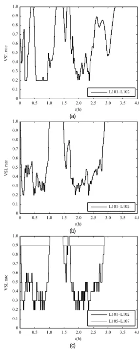
The resulting TTS for this scenario is equal to 9,315 veh·h, which is a 34.2 percent improvement compared to the no-control scenario. The related density and ramp queue profiles are shown in Figure 5(e-f), while the VSL rate tra-jectory at L101-L102 is shown in Figure 7(b). The density and flow at the bottleneck area are shown by the light gray curves in Figure 6.
Once again, it can be seen in Figure 5(e) that there are two congestions forming. In contrast to the two previous scenarios, the bottleneck congestion and, consequently, the capacity drop are completely avoided in the merge area of A1 (Figure 6(a)) as density remains around the set-point
value ρˆout ≈ρcr,L107 marked by the dotted line in the figure. The VSL rates at the application area (Figure 7(b)) are seen to go as low as 0.2, so as to hold back traffic. Because feedback maintains the density at the bottleneck around the set-point, the flow at that location (Figure 6(b)) is higher for feedback than for optimal control when the latter allows for a merge congestion to form.
Despite the fact that feedback has a higher flow at the bottleneck location than AMOC, the feedback control TTS is 5 percent higher (Table 1). A reason why feedback has a worse performance than AMOC is the BOR effect on far-ther upstream ramps. Note that, despite the local application of MTFC via VSLs at links L101-L102, AMOC acts with global network knowledge. This renders AMOC capable of managing the densities upstream of the bottleneck location in the most efficient way, so as to maximize throughput through all network off-ramps.
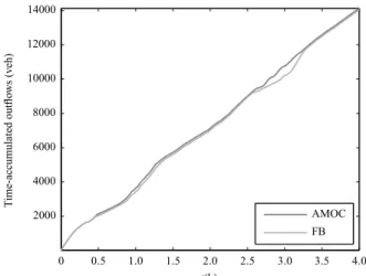
To better illustrate the BOR effect, Figure 8 shows, as an
(a)
(b)
(c)
Figure 7. VSL rate trajectories: (a) optimal control; (b)
feed-back control without constraints; and (c) feedfeed-back control with constraints
example, the time-accumulated outflow at the off-ramp to the A4 freeway that is clearly covered by both congestions forming in the no-control and feedback scenarios, but only covered by the first congestion in the AMOC case. At around t=0.5 h, the AMOC curve departs from the feed-back control curve, which indicates that more cars exited through DA4 in the AMOC case. The curves catch up with each other again at around t=2.5 h, but just after, the exit flow is again higher with AMOC.
The practicality of the feedback control approach pre-sented depends on the consideration of some operational requirements and constraints as introduced in Section 3.2.3. The VSL-induced critical density resulting from the VSL rate of 0.9 at the acceleration and bottleneck areas (L105-L107) is used as the set-point for the primary controller and is ρ =ˆout 34 veh/km/lane. The resulting TTS for this scenar-io is equal to 9,184 veh·h, which is a 35.2 percent im-provement compared to the no-control scenario and slightly better than the previous scenario. The detailed results are omitted, as the differences with the previous scenario are minor. The VSL rate trajectories at L101-L102 and L105-L107, however, are shown in Figure 7(c) and describe a similar trajectory as in the previous scenario while exhibit-ing discrete values as discussed in Section 3.2.3.
Typically, for safety reasons, additional VSLs may be applied upstream of the application area (see Section 3.2.3). In this case, the resulting TTS is equal to 9,513 veh·h, which is a 32.8 percent improvement compared to the
no-control scenario and slightly worse than the previous sce-narios. This efficiency reduction is considered minor in face of the potential safety benefits. Further details on the im-plementation of the operational restrictions can be found in Carlson et al. (2011a).
4.5. Sensitivity to variations of the parameters of the feedback controller
The gains used for the feedback controller in Section 4.4 were obtained using the zone-based method (Ellis, 2004; Carlson et al., 2011a). However, given the complexity of the system being dealt with, it is likely that a fine-tuning will still be required. Fine-tuning may be a complicated and time-consuming task, and, having a controller that exhibits a good performance for a range of its parameter values, may reduce the associated task burden. This is related to the problem of controller fragility analysis (Alfaro, 2007), i.e., how the performance of a control system is affected by var-iations of the parameters of the controller.
The performance of the system was evaluated by repeat-ing the first simulation of Section 4.4 for different combina-tions of parameters with values around the “nominal” values obtained in the first tuning of the controller. The sets used were KP′ ∈
{
34, 35,, 38,, 42, 43}
km/h and{
}
I′ ∈ 4, 5,, 9,, 13, 14
K km/h for the primary
control-ler, and KI∈
{
0.0010, 0.0011,, 0.0015,...,}
0.0019, 0.0020 h·lane/veh. The worst performance in terms of TTS resulted in a TTS of 9596 veh·h, i.e., an im-provement of 32.2 percent, obtained with KP′ =33 km/h,
I′ =14
K km/h and KI =0.0010 h·lane/veh. The best per-formance resulted in a TTS of 9258 veh·h, i.e., an im-provement of 34.7 percent, obtained with KP′ =37 km/h,
I′ =8
K km/h and KI =0.0020 h·lane/veh. In both cases the improvement is very close to the one obtained in Section 4.4 of 34.2 percent. Figure 9(a) shows the typical plot shape that was obtained for parameter sets where KI′ was kept fixed (in the figure, KI′ =11 km/h) and the other two pa-rameters (K and P′ KI) were varied as defined previously. An improvement is seen in the performance for increasing
P′
K and KI with an associated slightly more nervous con-trol action (not shown), though still within acceptable limits, i.e., the impact on traffic within and upstream of the appli-cation area is not compromised. In other words, the more Figure 8. Optimal and feedback control: time-accumulated
out-flows at off-ramp DA4
(a) (b)
Figure 9. Variation of the parameters of the feedback controller (a) TTS for KI′ =11 km/h and combination of values for KP′ and KI (b) density at the bottleneck location for the “nominal”, worst and best cases
limit than exhibited in Figure 7(c). In Figure 9(b) the densi-ty at the bottleneck area is shown for the worst and best cas-es as well as for the “nominal” case. There is no significant difference between the nominal and best cases. The worst case on the other hand, responds slightly slower and shows some stronger variations around the set-point.
5. CONCLUSIONS
This paper demonstrated the use of automatic control meth-ods applied to the mainstream traffic flow control (MTFC) on freeways. Two approaches, based on optimal and feed-back control methods, respectively, were reviewed and test-ed in simulation using a validattest-ed macroscopic second-order traffic flow simulator and a large-scale network model with realistic demands. Control was applied locally, and the results have shown that feedback control performs satisfac-torily. The performance of the closed-loop system was shown to have low sensitivity to variations of the parame-ters of the feedback controller, indicating that the possibly necessary fine-tuning in field applications is likely to not be too demanding. The feedback controller is deemed to be suitable for applications in the field.
Further improvements in total time spent could be ob-tained by the extension and integration of these controllers with other freeway control strategies and measures at the lo-cal and network-wide levels. Ongoing research is address-ing these problems and preliminary results can be found in Carlson et al. (2011b, 2012). A field test of the presented feedback strategy should be attempted in the near future.
ACKNOWLEDGEMENTS
The first author was supported by CAPES during part of the development of this research. For the research leading to these results, the co-authors have received funding from the European Research Council under the Eu-ropean Union's Seventh Framework Programme (FP/2007-2013)/ERC Grant Agreement n. 321132.
REFERENCES
Alessandri, A., A. Di Febbraro, A. Ferrara and E. Punta (1998) Optimal Control of Freeways via Speed Signalling and Ramp Metering.
Control Engineering Practice, v. 6, n. 6, p. 771–780. DOI:
10.1016/S0967-0661(98)00083-5.
Alfaro, V. M. (2007) PID Controllers’ Fragility. ISA Transactions, v. 46, n. 4, p. 555–559. DOI: 10.1016/j.isatra.2007.03.006.
Carlson, R. C., D. Manolis, I. Papamichail and M. Papageorgiou (2012) Integrated Ramp Metering and Mainstream Traffic Flow Control of Motorways Using Variable Speed Limits. Procedia - Social
and Behavioral Sciences, v. 48, p. 1578-1588. DOI: 10.1016/
j.sbspro.2012.06.1133.
Carlson, R. C., I. Papamichail and M. Papageorgiou (2013) Comparison of Local Feedback Controllers for the Mainstream Traffic Flow on Freeways Using Variable Speed Limits. Journal of Intelligent
Transportation Systems: technology, planning, and operations,
v. 17, p. 268-281. DOI:10.1080/15472450.2012.721330. Carlson, R. C., I. Papamichail and M. Papageorgiou (2011a) Local
Feed-back-based Mainstream Traffic Flow Control on Motorways Us-ing Variable Speed Limits. IEEE Transactions on Intelligent
Transportation Systems, v. 12, n. 4, p. 1261–1276. DOI:
10.1109/TITS.2011.2156792.
Carlson, R. C., I. Papamichail, M. Papageorgiou and A. Messmer (2010a) Optimal Mainstream Traffic Flow Control of Large-scale Motor-way Networks. Transportation Research Part C: Emerging
Technologies, v. 18, n. 2, p. 193–212. DOI: 10.1016/j.trc.2009.
05.014.
Speed Limits and Ramp Metering. Transportation Science, v. 44, n. 2, p. 238–253. DOI: 10.1287/trsc.1090.0314.
Carlson, R. C., A. Ragias, I. Papamichail and M. Papageorgiou (2011b) Mainstream Traffic Flow Control of Merging Motorways Using Variable Speed Limits. Proceedings of The 19th Mediterranean
Conference on Control and Automation. Corfu, Greece, p. 674–
681. DOI: 10.1109/MED.2011.5983115.
Chiang, Y. H. and J. C. Juang (2008) Control of Freeway Traffic Flow in Unstable Phase by H-infinity Theory. IEEE Transactions on
In-telligent Transportation Systems, v. 9, n. 2, p. 193–208. DOI:
10.1109/TITS.2008.922875.
Chung, K., J. Rudjanakanoknad and M. Cassidy (2007) Relation Between Traffic Density and Capacity Drop at Three Freeway Bottlenecks.
Transportation Research Part B: Methodological, v. 41, n. 1, p.
82–95. DOI: 10.1016/j.trb.2004.12.001.
Ellis, G. (2004) Control System Design Guide: a practical guide. Elsevier Academic Press, Amsterdam.
European Comission (2011) Roadmap to a single European transport
ar-ea – towards a competitive and resource efficient transport sys-tem. European Comission, Brussels, Belgium.
Gazis, D. C. and R. S. Foote (1969) Surveillance and Control of Tunnel Traffic by an On-line Digital Computer. Transportation Science, v. 3, n. 3, p. 255–275. DOI: 10.1287/trsc.3.3.255.
Greenberg, H. and A. Daou (1960) The Control of Traffic Flow to Increase Flow. Operations Research, v. 8, n. 4, p. 524–532.
Hegyi, A. and S. P. Hoogendoorn (2010) Dynamic Speed Limit Control to Resolve Shock Waves on Freeways - Field Test Results of the SPECIALIST Algorithm. 13th International IEEE Conference on
Intelligent Transportation Systems. Funchal, Madeira Island,
Por-tugal, p. 519–524. DOI: 10.1109/ITSC.2010.5624974.
Hegyi, A., B. De Schutter and H. Hellendoorn (2005) Model Predictive Control for Optimal Coordination of Ramp Metering and Varia-ble Speed Limits. Transportation Research Part C: Emerging
Technologies, v. 13, n. 3, p. 185–209. DOI: 10.1016/j.trc.
2004.08.001.
IEEE (2011) The Impact of Control Technology. Available at: <http://www.ieeecss.org>. (Accessed: 05/19/2012).
Isermann, R. (2011) Perspectives of Automatic Control. Control
Engi-neering Practice, v. 19, n. 12, p. 1399–1407. DOI: 10.1016/j.
conengprac.2011.08.004.
Kotsialos, A., M. Papageorgiou, C. Diakaki, Y. Pavlis and F. Middelham (2002a) Traffic Flow Modeling of Large-scale Motorway Net-works Using the Macroscopic Modeling Tool METANET. IEEE
Transactions on Intelligent Transportation Systems, v. 3, n. 4, p.
282–292. DOI: 10.1109/TITS.2002.806804.
Kotsialos, A., M. Papageorgiou, M. Mangeas and H. Haj-Salem (2002b) Coordinated and Integrated Control of Motorway Networks via Non-linear Optimal Control. Transportation Research Part C:
Emerging Technologies, v. 10, n. 1, p. 65–84. DOI: 10.1016/
S0968-090X(01)00005-5.
Lin, P.-W., K.-P. Kang and G.-L. Chang (2004) Exploring the Effective-ness of Variable Speed Limit Controls on Highway Work-zone Operations. Journal of Intelligent Transportation Systems, v. 8, n. 3, p. 155–168. DOI: 10.1080/15472450490492851.
Messmer, A. and M. Papageorgiou (1990) METANET: a Macroscopic Simulation Program for Motorway Networks. Traffic
Engineer-ing and Control, v. 31, n. 8, p. 466–470.
Papageorgiou, M., E. Kosmatopoulos and I. Papamichail (2008) Effects of Variable Speed Limits on Motorway Traffic Flow.
Transporta-tion Research Record: Journal of the TransportaTransporta-tion Research Board, v. 2047, p. 37–48. DOI: 10.3141/2047-05.
Papageorgiou, M. and A. Kotsialos (2002) Freeway Ramp Metering: an Overview. IEEE Transactions on Intelligent Transportation
Sys-tems, v. 3, n. 4, p. 271–281. DOI: 10.1109/TITS.2002.806803.
Papamichail, I., A. Kotsialos, I. Margonis and M. Papageorgiou (2010) Coordinated Ramp Metering for Freeway Networks – a Model-predictive Hierarchical Control Approach. Transportation
Re-search Part C: Emerging Technologies, v. 18, n. 3, p. 311–331.
DOI: 10.1016/j.trc.2008.11.002.
Popov, A., R. Babuska, A. Hegyi and H. Werner (2008) Distributed Con-troller Design for Dynamic Speed Limit Control Against Shock Waves on Freeways. Proceedings of The 17th IFAC World
Con-gress. Seoul, Korea, p. 14060–14065. DOI:
10.3182/20080706-5-KR-1001.02380.
Schrank, D., T. Lomax and S. Turner (2010) Urban Mobility Report 2010. Texas Transportation Institute, The Texas A&M University
Sys-tem. Available at: <http://mobility.tamu.edu>. (Accessed: 01/22/2011).
Zhang, J., H. Chang and P. A. Ioannou (2006) A Simple Roadway Control System for Freeway Traffic. 2006 American Control Conference. Minneapolis, MN, USA, p. 4900–4905. DOI: 10.1109/ACC. 2006.1657497.