UNIVERSIDADE DE LISBOA
FACULDADE DE CIÊNCIAS
DEPARTAMENTO DE BIOLOGIA ANIMAL
EFFECTS OF SEED AVAILABILITY
ON EURASIAN RED SQUIRREL (SCIURUS VULGARIS)
LIFE-HISTORY AND DEMOGRAPHIC PARAMETERS
IN TWO PINE FORESTS IN THE ITALIAN ALPS
UNIVERSIDADE DE LISBOA
FACULDADE DE CIÊNCIAS
DEPARTAMENTO DE BIOLOGIA ANIMAL
EFFECTS OF SEED AVAILABILITY
ON EURASIAN RED SQUIRREL (SCIURUS VULGARIS)
LIFE-HISTORY AND DEMOGRAPHIC PARAMETERS
IN TWO PINE FORESTS IN THE ITALIAN ALPS
Dissertação orientada por:
Professor Doutor Lucas A. Wauters
Professora Doutora Maria da Luz Mathias
Acknowledgments
To all the people who have contributed and made this work possible, I hereby express my sincere gratitute, particularly to:
Dr. Lucas A. Wauters, for his supervision, concern, advice and unconditional support during the preparation and writing of this dissertation and for revising the final version.
Dra. Maria da Luz Mathias, for accepting the internal supervision of this work, being always available and supportive during the whole process.
Ambrogio Molinari, for his availability, support and companionship and for being the best field teacher and colleague anyone could ever have.
All the colleagues with whom I shared the field work and countless freezing hours: Nuno Oliveira, Claudia Romeo, Francesco Bisi, Serena and Federico, because we survived the Alps.
Anne Ghisla, for her availability, patience and priceless help with the R program and geographic data analyses.
All the people at Dipartimento Ambiente-Salute-Sicurezza of the Università degli Studi dell’Insubria, specially Adriano Martinoli, Damiano Preatoni, Francesco Bisi, Elisa Masseroni, Alessio Martinoli, Martina Spada and Mosè Nodari, for all the help and expert opinions in alpine ecology and biology in general and for really making me feel like part of a biologists team.
All my friends, specially my Erasmus family: Isabel Neves, Nuno Oliveira, António Ferreira, Carina Seewald, Carlos Cuervo, Juan Jiménez, Laura Menacho, Juliana Perdomo, Ana Castro, Carlos Aguado, Isabel Navarro, Lorena Cabrera and Mattia Castiglioni, for providing me with the most unforgettable moments of this entire year and for being like a comfortable place where I always feel welcome.
Carlo, for the love and the friendship, for sharing the good moments, for the support in bad moments, for always being interested in what I do and making me feel like I can accomplish anything.
Resumo
A substituição em larga escala do nativo esquilo-vermelho Euro-asiático (Sciurus vulgaris) pelo introduzido esquilo-cinzento Norte-americano (Sciurus carolinensis) exemplifica um caso de competição interespecífica, por parte de uma espécie introduzida invasiva. Até há pouco tempo, o risco de extinção do esquilo-vermelho estava limitado às Ilhas Britânicas mas actualmente, com o estabelecimento do esquilo-cinzento no Norte de Itália, esta problemática pode potencialmente atingir todo o continente europeu se a espécie introduzida ultrapassar os Alpes.
Diversos estudos parecem indicar que o esquilo-vermelho beneficia da presença de vastas extensões de florestas de coníferas, estando melhor adaptado que o esquilo-cinzento para se alimentar das pequenas, e difíceis de extrair, sementes destas árvores. Deste modo, as florestas de coníferas alpinas podem constituir um refúgio para o esquilo-vermelho contra a expansão do cinzento e representar o único habitat no Norte de Itália e países adjacentes onde o esquilo-vermelho terá algumas probabilidades de sobrevivência a longo prazo. Contudo, não é possível testar directamente esta hipótese uma vez que a distribuição do esquilo-cinzento ainda não atingiu a região alpina. O Dipartimento Ambiente-Salute-Sicurezza da Università degli Studi dell’Insubria (em colaboração com a Università degli Studi di Torino) encontra-se, desde 1999, a promover um programa de investigação (ASPER - Alpine Squirrel Population Ecology Research) sobre o papel do esquilo-vermelho no ecossistema das florestas alpinas, no qual este estudo se insere.
Em sistemas de recursos limitados, com um elevado nível de variação temporal na qualidade dos habitats, os parâmetros demográficos e de história de vida de pequenos mamíferos são principalmente afectados pela distribuição e defesa de recursos essenciais. Estes parâmetros estão bem documentados em habitats óptimos e sub-óptimos. Contudo, devido às dificuldades de estudar populações de pequenas densidades, as relações alimentação – uso do espaço – dinâmica populacional são ainda pouco compreendidas em habitats extremos ou de pouca qualidade. Do mesmo modo, pouco se sabe sobre a existência de possíveis adaptações no tamanho/peso do corpo e outros parâmetros de história de vida de indivíduos em habitats extremos e, mais ou menos, isolados.
corporal dos esquilos e as densidades populacionais. Assumiu-se que CAN é um habitat marginal devido a determinadas características como: Invernos frios e longos com cobertura permanente do solo pela neve; uma única fonte de recursos alimentares, as sementes de pinheiro-montanhês (Pinus mugo), de baixa taxa de assimilação de energia (os esquilos demoram muito tempo a manusear as pequenas pinhas para se alimentarem das sementes) e um elevado nível de variação temporal na disponibilidade alimentar devido às marcadas flutuações anuais na produção de sementes. Os dados recolhidos em BOR, uma floresta mista de coníferas próxima, dominada pelo pinheiro-suíço-das-rochas (Pinus cembra), sujeita a condições climatéricas semelhantes, foram utilizados como comparação com CAN. BOR não é considerado um habitat marginal porque o conteúdo energético específico das sementes das suas coníferas é elevado, esperando-se uma elevada taxa de assimilação de energia pelos esquilos. Sendo assim, previu-se para CAN: (1) recursos alimentares mais escassos; (2) densidade populacional e proporção de fêmeas reprodutivas mais baixas; (3) esquilos mais pequenos e magros; (4) áreas vitais e suas core areas de maior tamanho; (5) maior sobreposição de core areas, especialmente entre fêmeas, visto que, nestas condições, não é proveitoso para as fêmeas defender territórios intrasexuais.
Estimou-se a produção média anual de sementes por espécie de conífera para cada área de estudo através da recolha de pinhas (número médio de sementes por pinha de cada espécie) e da contagem do número de árvores de cada espécie de conífera, em áreas de amostragem em BOR e CAN. A produção média anual de sementes por espécie foi convertida em valores energéticos para possibilitar a combinação de dados de diferentes espécies, permitindo a estimativa da disponibilidade alimentar em cada área de estudo.
Utilizou-se o método de Captura – Marcação – Recaptura durante 3 períodos distintos, em ambas as áreas de estudo: Abril-Maio, Junho-Julho e Setembro de 2006 e 2007, durante 8-12 dias até não se capturarem animais novos por 2 dias consecutivos. A informação recolhida nas capturas dos esquilos foi: sexo, idade, peso, comprimento da pata posterior direita (tamanho), condição reprodutiva, fase cromática do pêlo e mudanças de fase. Na maioria dos indivíduos adultos capturados foram colocados colares radiotransmissores para estudar o comportamento espacial individual e procurar ninhos de fêmeas em lactação, usando telemetria (em 2006, apenas em CAN, por razões logísticas, e em 2007, em ambas as áreas). O número mínimo conhecido de animais vivos (MNA) das capturas, telemetria e observações durante cada período de captura foi utilizado como uma estimativa das densidades populacionais.
Outono. Em 2007, 6 animais foram monitorizados em CAN durante a Primavera-Verão e 7 durante o Outono. No mesmo ano, 8 animais foram monitorizados em BOR durante a Primavera-Verão e 6 durante o Outono. Em cada período e para cada animal monitorizado, os seguintes parâmetros foram calculados: área vital total (100% das localizações) através do método do Mínimo Polígono Convexo (100% MCP); 95% da área vital (95% das localizações) usando o método de Kernel (95% KDE); estimativa da core area, baseada em 85% da área vital, usando o método Kernel (85% KDE); sobreposição de core areas masculinas, expressa como a % de sobreposição da core area de cada macho com as core areas de todos os outros machos; sobreposição de core areas femininas, expressa como a % de sobreposição da core area de cada fêmea com as core areas de todas as outras fêmeas; fidelidade ao local, estimada como a % média da sobreposição das core areas da Primavera-Verão e do Outono.
Algumas das diferenças previstas entre os parâmetros demográficos e de história de vida das duas populações de esquilos-vermelhos estudadas, baseadas na hipótese de CAN ser um habitat marginal, não foram concretizadas. A previsão (1) foi confirmada apenas para 2007, quando a disponibilidade de sementes das coníferas foi mais baixa para CAN do que BOR (464.8 e 1403.9 MJ ha-1, respectivamente). Os dados recolhidos durante estes 2 anos sugerem que a abundância alimentar em CAN é semelhante à de BOR, quando o Pinus cembra apresenta uma produção pobre e não existe um excesso de produção de Picea abies, enquanto uma produção média-alta de Pinus cembra resulta numa maior abundância alimentar em BOR que CAN.
As previsões (4) e (5) foram confirmadas: os esquilos-vermelhos usaram áreas vitais e core
areas maiores, e ocorreu maior sobreposição de core areas, em CAN do que BOR (100% MCP,
17.9 e 6.6 ha; 95% KDE, 33.2 e 9.1 ha; 85% KDE, 30.1 e 9.1 ha, respectivamente), apesar do esperado aumento na sobreposição de core areas das fêmeas não ser significativo. Como era esperado, a baixa densidade de sementes de coníferas em CAN forçou os esquilos de ambos os sexos a aumentar o tamanho das suas áreas vitais e core areas e a sobreposição de core areas, de modo a encontrarem alimentos suficientes para alcançar as suas necessidades energéticas. A sobreposição de core areas das fêmeas pode não ter sido significativa devido a um pequeno número de amostras e/ou a uma elevada variação entre fêmeas no nível de sobreposição de core
energia em ambas as áreas de estudo, de forma a produzir uma hipótese mais específica para a relação entre a ingestão de alimentos e as densidades populacionais. As semelhanças no tamanho e peso do corpo dos esquilos-vermelhos em ambas as áreas de estudo sugerem que as pressões selectivas nestes caracteres não diferem fortemente nestes dois habitats. Será necessária uma monitorização da variação anual no peso dos esquilos durante um período de tempo mais longo, para investigar que factores ambientais, por exemplo, condições climatéricas ou acesso limitado a sementes das coníferas, principalmente no Inverno-Primavera, afectam os padrões de variação do peso dos esquilos nestas duas áreas de estudo.
Os resultados obtidos sugerem que não existe uma diferença marcada na qualidade dos habitats entre CAN e BOR e que este último também se pode “comportar” como um habitat marginal em anos de baixa produção pelas coníferas (sendo um habitat de média qualdidade em anos de boa produção pelas coníferas). Apesar das dificuldades logísticas de estudar a população de BOR durante o Inverno, a investigação futura deve recorrer a estudos de longo prazo (superiores a 5 anos) durante todas as estações do ano, em ambas as áreas de estudo. Devem também recorrer à comparação entre parâmetros demográficos e de história de vida das populações de BOR e CAN com populações em outros tipos de florestas alpinas, que ocorrem a altitudes mais baixas e são caracterizadas por diferentes padrões temporais na disponibilidade de sementes de coníferas e sua abundância.
Palavras-chave:
Rodentia, florestas alpinas, habitat marginal, disponibilidade alimentar, área vital, telemetria, densidade populacional.Summary
In North Italy, the Eurasian red squirrel (Sciurus vulgaris) is threatened by the expansion of the introduced, invasive North-American grey squirrel (Sciurus carolinensis). Alpine conifer forests might constitute a stronghold for the long-term persistence of red squirrel populations in North Italy and adjacent countries.
In resource limited systems, with a high degree of temporal variation in habitat quality, as Alpine conifer forests, the distribution and defensibility of critical resources are the main factors affecting life-history and demographic parameters of squirrels, which are still poorly understood in these more or less isolated and extreme habitats. In the present study, variation in tree-seed availability, red squirrels population densities, body size and mass and spacing patterns were monitored over different seasons in 2006 and 2007, to explore how differences in food availability between two alpine pine forests, Bormio (BOR) and Cancano (CAN), affected the behaviour and body condition of individual squirrels and the population densities, assuming that CAN was a marginal habitat contrary to BOR which was not one.
Only in 2007, food availability was significantly different in the study sites, with seed-crop size being three times bigger at BOR than CAN. Red squirrels used larger home ranges and core areas and had a higher core area overlap at CAN than BOR, as predicted due to the need to meet daily energy-requirements. However, the expected increase in female-female core area overlap in CAN was not significant. Annual squirrel densities (BOR, 0.13 and 0.20 squirrels ha-1; CAN, 0.10 and 0.18 squirrels ha-1) and proportion of reproducing females were similar in both study sites and so was body mass, in contradiction with predictions that assumed lower density and body mass values for Cancano.
These results suggest that there is no marked difference in habitat-quality between CAN and BOR and that the latter “behaves” as a marginal habitat in years with poor pine-crops but as a medium-quality habitat in years of good pine-crops. Despite the logistic difficulties, future research should comprise long-term monitoring in both study sites and the comparison of life-history and demographic parameters from these populations with populations in other types of
Index
Acknowledgments I
Resumo II
Summary VI
1. Introduction 1
1.1. The study-system: red squirrels in high-elevation conifer forests 3
2. Materials and Methods 6
2.1. Study sites 6
2.2. Estimating seed availability 9 2.3. Trapping and handling squirrels 11 2.4. Radio-tracking and space use analysis 13
2.5. Statistical analyses 15
2.5.1. Estimating seed availability 15 2.5.2. Body size and body mass analysis 15 2.5.3. Space use analysis 16
3. Results 17
3.1. Estimating seed availability 17 3.2. Squirrel population densities 17 3.2.1. Female reproduction 20 3.3. Body size and body mass analysis 21 3.3.1. Variation in foot length of subadult and adult squirrels 23 3.3.2. Variation in body mass of subadult and adult squirrels 23
3.4. Space use analysis 25
3.4.1. Core area overlap 28
3.4.2. Site fidelity 30
4. Discussion 31
4.1. Variation in seed availability 31 4.2. Variation in squirrel population densities 32 4.3. Variation in squirrel body size and mass 34 4.4. Variation in squirrel home range and core area size 36 4.5. Variation in squirrel core area overlap 38
1. Introduction
Safeguarding the Earth’s diversity is the best way to maintain our life support system. There is evidence to suggest that the biosphere acts as a self-regulating whole and that diverse systems may be more resilient than less diverse systems (e.g., Lowe et al. 2000).
In many ecosystems, the introduction of invasive alien species is a major threat for the maintenance of biodiversity (e.g., CBD 1992; Millennium Ecosystem Assessment 2005; Hulme 2006). It is claimed to be second only to the destruction and fragmentation of natural habitats as a cause of population reduction and extinction of native species, in the regions where the aliens have been introduced (Mack et al. 2000; Millennium Ecosystem Assessment 2005). Invasive alien species can interfere with the native fauna by different ecological processes, such as predation, interspecific competition or acting as vector of diseases (Ragg et al. 1995; Alterio et al. 1998; Gurnell et al. 2004; Rushton et al. 2006).
For example, the Nile perch (Lates niloticus) was introduced to Lake Victoria, Africa, in 1954 and since then, has contributed to the extinction of more than 200 endemic fish species through predation and competition for food. The far-reaching impacts of this introduction have been devastating for the environment as well as for communities that depend on the lake (Lowe et
al. 2000; Goudswaard et al. 2008). There is also the small Indian mongoose (Herpestes javanicus auropunctatus) which was introduced to Mauritius, Fiji, West Indies and Hawaii in the late 1800s
to control rats. Island populations of native fauna, which had evolved without the threat of a fast-moving, mammalian predator, were no match for the mongoose. It has caused the local extinction of several endemic birds, reptiles and amphibians besides being a vector of rabies (Lowe et al. 2000; Watari et al. 2008).
Therefore, these introduced species not only present a serious ecological problem but often also a socio-economical and political one (Bertolino & Genovesi 2003; Born et al. 2005). Many alien species cause direct economic damage to human activities (farming, forestry, zoo-technology, disease risk), but nevertheless their control often becomes an emotional issue, in particular with mammal pest species (White & Whiting 2000; Bertolino & Genovesi 2003).
The Eurasian red squirrel is the only native European tree squirrel. Its favourite habitats are the large blocks of conifer forests of northern Europe and Alpine forests, but this species has a widespread distribution from western Europe to northeast China (Macdonald & Barrett 1993).
Red squirrels have become replaced by grey squirrels in nearly all broadleaf woodlands in the British Isles (Reynolds 1985; Gurnell et al. 2004). Considered a pest by 1930, there have been various attempts over the years to control or eradicate the grey squirrel in the UK (Genovesi 2005). Also in northern Italy, after introduction of the grey squirrel in Piemonte (1948) and Liguria (1966) (Currado 1997), recent investigations revealed that its distribution is in continuous expansion, in direction to prealpine forests, leading to red squirrels disappearance from the range currently occupied by grey squirrels (Currado 1997; Wauters et al. 1997; Lurz et al. 2001; Tattoni
et al. 2006). Until a few years ago, the extinction risk for red squirrels was limited to the British
Isles but now, with the establishment of grey squirrels in North Italy, this problem can potentially involve all of the European continent, if the introduced species is able to pass the Alps (Lurz et al. 2001; Tattoni et al. 2006).
Political concern about the lack of action in many countries has been expressed by the Permanent Commision of the Bern Convention, which has produced several recommendations (n. 57 and 77 of 1997) urging countries to eradicate alien invasive species where possible. A specific recommendation to the Italian authorities (n. 78 of 1997) underlines the necessity to eradicate grey squirrels in order to stop the species’ further diffusion in Europe, and save the native red squirrel from wide-scale extinction. An eradication campaign was started in Italy in 1997 but was suspended following legal action by some radical animal rights organisations (Genovesi & Bertolino 2001). The suspension of activities was followed by a significant range expansion of the grey squirrel (Genovesi 2005).
Red squirrels are being replaced by greys through interspecific competition for the same food resources, leading to competitive exclusion, which acts mainly on juveniles (Wauters & Gurnell 1999; Wauters et al. 2001a, 2002a, b), and, in the UK, through the transmission of a virus disease (poxvirus) (Rushton et al. 2006).
Accordingly, the grey squirrel was considered by the Invasive Species Specialist Group of IUCN, one of the world’s 100 worst invasive alien species (Lowe et al. 2000), for the impacts it provokes: extinction of red squirrels, impact on birds and other wildlife(Gurnell & Mayle 2003), vector for poxvirus and damages to hardwood timber through bark stripping activity, resulting in
of these trees (Lurz et al. 1995; Kenward et al. 1998; Molinari et al. 2006). Therefore, Alpine conifer woodlands may constitute a stronghold for red squirrels against the expansion of greys, and represent the only habitat in Italy and adjacent countries, in which red squirrels have some probabilities of long-term survival. Currently, this can not be proved directly because grey squirrels have not yet arrived to the Alps.
To understand the population status and ecological niche of native red squirrels in Alpine forests, we need a better knowledge of population consistency, population dynamics, demographic processes (such as reproduction, survival, immigration, emigration) and spacing behaviour of red squirrels in the various types of Alpine conifer woodlands. The Dipartimento Ambiente-Salute-Sicurezza of the Università degli Studi dell’Insubria (in colaboration with the Università degli Studi di Torino) is, since 1999, carrying out an investigation program (ASPER - Alpine Squirrel Population Ecology Research) about the role of the red squirrel in the Alpine forests ecosystem, in which this study is inserted.
1.1. The study-system: red squirrels in high-elevation conifer forests
In resource limited systems with a high degree of spatial variation in habitat quality, the spacing behaviour and population dynamics of small mammals are mainly affected by the distribution and defensibility of critical resources (Maher & Lott 1995, 2000).
Spacing behaviour and habitat use, especially of adult breeding females, will not only influence individual variation in reproductive success, but also overall population growth and density (Boyce & Boyce 1988; Wauters & Dhondt 1995; Wauters & Lens 1995; Wauters et al. 1995, 2001b). Therefore, understanding relationships between spatial variation of food supplies and spacing behaviour and reproductive output is of general interest to ecologists.
Squirrels are good model organisms to study the producer-consumer relationships in temperate forests of Europe, since they strongly depend on the availability of tree seeds. Conifer tree-seed production is a typical example of a pulsed resource and when important food resources are produced in pulses (high annual variation in seed-crop size), different potential responses by the consumer (in this case the seed predator, the red squirrel) can be predicted (Boutin et al. 2006).
The spacing behaviour of Holarctic tree squirrels and its effects on population processes are well documented in optimal and sub-optimal habitats (Rusch & Reeder 1978; Kenward 1985; Wauters & Dhondt 1992; Larsen & Boutin 1994; Lurz et al. 1997, 2000; Selonen et al. 2001; Wauters et al. 1995, 2001b, 2002a, 2005; Di Pierro et al. 2008). However, because of the difficulties of studying populations at low densities, the food - space use - population dynamics relationships in extreme or poor-quality habitat types are still poorly understood. Likewise, little is known about possible local adaptations in body size and/or life-history traits to (more or less isolated) extreme habitats.
The studies, concerning red squirrels in the Alpine ecosystem, which have been made, consider such aspects as red squirrels parasites (Bertolino et al. 2003; Kvac et al. 2008), food preferences (Bertolino et al. 2004, Molinari et al. 2006), genetic structure (Trizio et al. 2005), coat-colour polymorphism (Wauters et al. 2004a), spacing behaviour (Wauters et al. 2005; Di Pierro et al. 2008) and effects of variation in food supply on fitness components (Wauters et al. 2007a) and demography (Wauters et al. 2008). Most of these studies were carried out in the last 8 years by the ASPER project.
One of the studies concerning spacing behaviour, aimed to investigate whether a model of spatial organization in vertebrates, the “space-use model”, could be extended to predict intra-population variation in space-use in a habitat with a strong temporal variation in resource abundance (Wauters et al. 2005). The second one, had the aim to investigate, in a more detailed way, intrasexual territoriality in red squirrels (Di Pierro et al. 2008).
In the present study, variation in tree seed availability, body size and mass of red squirrels, population densities and spacing patterns were monitored over different seasons and years, to explore how differences in food availability between two alpine pine forests (Bormio and Cancano) affected the behaviour and body condition of individual squirrels and the population density.
It was assumed that dwarf mountain pine woodland (Cancano) is a marginal habitat, because it is characterised by: (1) long, cold winters with permanent snow cover; (2) a single major food resource, pine seeds from dwarf mountain pine, with a low rate of energy-intake (relatively long handling times to consume the pine seeds from small cones); and (3) a high degree of temporal variation in food availability due to marked annual fluctuations in seed production.
Using this hypothesis, it was predicted that at Cancano:
(1) seed-crop size will be smaller and hence food resources will be scarser;
(2) if food limits density and/or reproductive rate, lower densities and a lower proportion of reproducing females than in other, less marginal habitats, will be expected;
(3) squirrels will be smaller or weigh less, since lack of food reduces body mass;
(4) at low levels of food resources, there will be an increase of home range size and core area size;
(5) core area overlap, especially among females, will increase strongly, since it will be no longer profitable for females to defend intrasexual territories.
Data gathered in a nearby Arolla pine forest (Bormio), which is not considered a marginal habitat and is subject to similar weather conditions, was used for comparison with the life-history and demographic parameters collected at Cancano. Theoretically, one can expect that this forest is a good habitat in most years, since cone-specific energy-content is high and squirrels should be able to have a high rate of energy-intake when there are medium-high seed-crops.
Although I worked in the ASPER program through the October of 2007 – July 2008 period, this study presents data, obtained in the same study sites and using the same methodology, from the 2006 and 2007 years, so it could be possible for me to analyse data from two complete years. Since the ASPER program aims to be a long-term monitoring of alpine red squirrel populations, the data I collected will be used in future studies of this multidisciplinary program.
2. Materials and Methods
2.1. Study sites
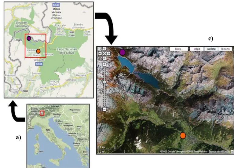
Red squirrels were monitored in two study sites in Parco Nazionale dello Stelvio in North-East Valtellina, Lombard Alps (Sondrio Province, Lombardia Region, Italy, see Figure 1).
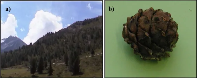
Study site Bormio (BOR, 46°27′N, 10°30′E, elevation 1,950–2,130 m a.s.l.) is a mature (trees are more than 40 years old), mixed subalpine conifer forest located south of the village of Bormio. It extends over 93 ha and is dominated by Arolla pine (Pinus cembra L., 73%), with scattered individuals of larch (Larix decidua Mill., 18%), Norway spruce (Picea abies (L.) H. Karst., 8%) and few dead trees (1%) (see Figure 2a, b). Arolla pine has large, wingless seeds and depends on birds (mainly nutcrackers, Nucifraga caryocatactes L., 1758) and squirrels for seed-dispersal. Theoretically, one can expect that this forest is a good habitat in most years, since cone-specific energy-content is high and squirrels should be able to have a high rate of energy-intake when there are medium-high seed-crops.Moreover, Norway spruce trees can, in some years, have a high and synchronised seed production (masting), with pines remaining available in the canopy for about 10 months.
Study site Cancano (CAN, 46º33´N, 10º15´E, elevation 1,950 m a.s.l.) is located at the bottom of a high-elevation valley near the artificial lakes of Cancano. It extends over 54 ha and is almost entirely composed of a pioneer homogeneous dwarf mountain pine (Pinus mugo Turra) woodland, whose seeds are dispersed by wind (see Figure 2c, d). The understorey consists mainly of winter heath (Erica herbacea L.), european blueberry (Vaccinium myrtillus L.), mountain cranberry (Vaccinium vitis-idaea L.) and common juniper (Juniperus communis L.). CAN has just this single major food resource for squirrels, pine seeds from dwarf mountain pine, with a low rate of energy-intake (relatively long handling times to consume the pine seeds from small cones).
Both sites are characterised by an altitude continental climate, typical of the Central Alps, with mean annual temperatures below 3ºC, relatively moderate precipitation, occurring mostly in summer, and long, cold winters resulting in a fixed period of 5 to 7 months snow cover each year (mean monthly temperatures below 0°C from November to April).
Figure 1. Maps: a) Italy, with Parco Nazionale dello Stelvio signalised (red); b) Parco Nazionale dello Stelvio, with
Bormio (orange) and Cancano (purple) study sites signalised and c) detail of the park with Bormio (orange) and Cancano (purple) study sites signalised, from Google Maps.
a)
b)
Figure 2. Photos: a) Bormio study site and b) pine from Arolla pine by Ambrogio Molinari; c) Cancano study site and
d) pines from dwarf mountain pine by Claudia Romeo.
a)
b)
2.2. Estimating Seed Availability
Woodland composition was determined by establishing a 20 m by 20 m (400 m2) vegetation plot, centred on each of the 20 and 31 trapping stations across BOR and CAN, respectively (see Figure 3). In each vegetation plot, the number of trees of each species was counted, and the diameter at breast-height (DBH in cm) of two randomly chosen mature trees, for each species on the plot, hereinafter called “sample trees”, was measured (Wauters et al. 2005). At CAN, shrubs and trees of dwarf mountain pine were counted separately.
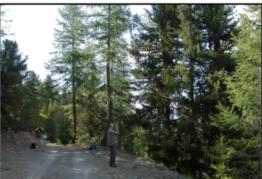
In July of each year (2006 and 2007), fresh cones of Arolla pine, larch, Norway spruce and dwarf mountain pine were counted in the canopy of all sample trees from a fixed position using 10x40 binoculars (see Figure 4). Counting was carried out during this period because the cones of the current year (new production) are fully developed and easily recognised, and only few cones have already been predated (Wauters et al. 2005; Salmaso et al. in press). In previous ASPER studies, 50 fresh cones of each tree species (max. two cones/tree) had been collected and the number of seeds in each single cone had been counted, to estimate average number of seeds per cone. This gave an estimate of annual seed production per tree species (cones tree-1 * mean seeds cone-1) in each vegetation-plot. To combine data from different seed species, number of seeds tree -1
was converted to energy values (kJ tree-1) by multiplying cones tree-1 with average cone-energy content. Mean energy-content per cone was estimated as described in Salmaso et al. (in press), by multiplying seed dry mass and caloric value (mean seed dry mass * kJ g-1 dry mass) with mean seeds cone-1. Values obtained were 121.3 kJ for Arolla pine, 9.4 kJ for larch, 51.0 kJ for Norway spruce and 5.7 kJ for dwarf mountain pine.
The number of trees of each species in each vegetation plot and the species-specific seed energy tree-1 was used to calculate seed availability per species and total seed availability in each vegetation plot (in MJ ha-1). The mean value of all vegetation plots was then used as the measure of average annual tree seed abundance per species and for all species combined (total tree seed abundance).
Figure 3. Images: a) Bormio and b) Cancano study sites, with the trapping stations signalised in red (20 and 31,
respectively), from Google Earth.
a)
Figure 4. Photo of the counting of fresh cones in the canopy of sample trees using 10x40 binoculars, by Claudia
Romeo.
2.3. Trapping and Handling Squirrels
In both study sites, trapping was carried out in three distinct periods: April-May, June-July and September, from April 2006 to September 2007. Captures were performed using ground-placed Tomahawk “squirrel” traps (models 201 and 202, Tomahawk Live Trap, WI, USA) baited with sunflower seeds and hazelnuts (see Figure 5a). For BOR and CAN, 20 and 31 traps were placed respectively, uniformly distributed according to a pre-established grid (see Figure 3). Traps were pre-baited with sunflower seeds and hazelnuts 4 to 6 times over a 30 days period, and then baited and set for 8-12 days, until no new, unmarked squirrels were trapped for at least 2 consecutive days. Trap controls were executed two times a day, during the end of morning and end of the afternoon, so that captured animals did not remain inside the traps for too much time.
Each trapped squirrel was flushed into a light cotton handling bag with a zipper or a wire-mesh “handling-cone” to minimise stress during handling (see Figure 5b) and individually marked using numbered metal ear-tags (type 1003 S, 10 by 2 mm, National Band and Tag, Newport, KY, USA). It was weighted to the nearest 5 g using a Pesola spring-balance (Pesola AG, Baar, Switzerland) and the length of right hind foot (without nail) was measured (0,5 mm) with a thin ruler (see Figure 5c) (Wauters & Dhondt 1989a, b, 1995). Sex, age-class, reproductive condition
1=anoestrus (vulva small, no longitudinal opening, not lactating); 2=oestrus (or post-oestrus, vulva partly or strongly swollen with longitudinal opening, enlarged belly during late pregnancy); or 3=lactating (nipples large, milk excretion can be stimulated, (Wauters & Dhondt 1995; Wauters & Lens 1995). Fur chromatic phase was scored as: 1=red morph, 2=intermediate morph, 3=black morph.
The majority of adult squirrels trapped in 2006 (only in CAN due to logistic problems) and in 2007 (in both sites) were fitted with radio-collars (model M1640, Advanced Telemetry System Inc., USA), to study individual spacing behaviour and look for nests of lactating females using radio-tracking (see Figure 5d).
The minimum number of animals known to be alive (MNA), from trapping, radio-tracking or observations, during each trapping period was used as an estimate of population size. Previous studies on a wide range of red squirrel populations showed that these estimates realistically represent true squirrel densities (e.g. Wauters et al. 2001b, 2004b, 2008; Wheatley et al. 2002).
a)
b)
2.4. Radio-tracking and Space Use Analysis
Radio-tracking consists on locating an animal fitted with a transmitter radio-collar, which periodically emits short radio impulses at a specific frequency, using a directional receiving antenna connected to a radio-receiver which transforms the radio signal in a sound signal and/or a visibly one, perceptible to the operator, who can then individualise the marked animal’s position. The radio-tracking technique used was homing-in, consisting on following the radio signal until the observation of the marked animal or individualisation of a limited presence area by the animal being pinpointed by signal strength and direction (see Figure 6a) (Kenward 1987; Wauters & Dhondt 1992; Di Pierro et al. 2008). Radio-collar signals were located using Wildlife radio receivers (model TRX-2000S, Wildlife Materials Inc., USA) and three elements directional Yagi antennas (see Figure 6b).
Red squirrels were monitored over 3-month periods within each season, with two or three radio-locations (fixes) per day. Seasonal variation in squirrel home ranges and patterns of habitat use were investigated for the following periods: spring-summer (May-July) and autumn (September-October). In 2006, 3 animals were monitored at CAN during spring-summer (2 males, 1 female) and 2 animals were monitored during autumm (1 male, 1 female). In 2007, 6 animals were monitored at CAN during spring-summer (3 males, 3 females) and 7 animals were monitored during autumm (3 males, 4 females). In the same year, 8 animals were monitored at BOR during spring-summer (5 males, 3 females) and 6 animals were monitored during autumm (4 males, 2 females).
For home range analysis, between 25 and 45 fixes were collected for each squirrel, which proved sufficient to adequately describe a squirrel’s home range (Wauters & Dhondt 1992; Wauters et al. 2001b, 2005). At each fix, the squirrel’s location (through GPS), activity (1=active, 2=in a nest) and position (on the ground or in a tree, determining tree species) were recorded.
Subsequently, data was recorded in a GIS database, and Arcview 3.2 (ESRI Inc. 1999; ESRI Inc. 2002) and R software (R Development Core Team 2007)were used to calculate home ranges. Two different methods were used for home range estimation: the Minimum Convex Polygon (Harris et al. 1990), to allow comparisons with previous studies, and the fixed Kernel
Andrén & Lemnell 1992; Wauters & Dhondt 1992; Lurz et al. 2000; Wauters et al. 2001b, 2005, 2007b; Di Pierro et al. 2008).
For each squirrel, in each period, the following parameters were calculated:
1) total home range area (100% of the fixes) using the Minimum Convex Polygon Method
(MCP) (Harris et al. 1990);
2) 95% home range area (95% of the fixes) using the fixed Kernel method (KDE 95%)
(Worton 1989);
3) core area estimate, based on the 85% core area using the fixed Kernel method (KDE 85
%) (Worton 1989);
4) male core area overlap, expressed as percentage of overlap of a squirrel’s core area with
the core area of all other male squirrels (Wauters & Dhondt 1992),
5) female core area overlap, expressed as percentage of overlap of a squirrel’s core area
with the core area of all other female squirrels (Wauters & Dhondt 1992),
6) site fidelity, estimated as the average % overlap of an individual’s spring-summer and
autumn core areas [fidelity = (% spring-summer core overlapped by autumn core + % autumn core overlapped by spring-summer core)/2].
Figure 6. Photos: a) performing radio-tracking by homing-in (by Diana Rodrigues) and b) needed material for
homing-in: radio receiver, Yagi antenna and GPS (by Ambrogio Molinari).
2.5. Statistical analyses
All statistical analyses were carried out using the SAS software (SAS 1999).
2.5.1. Estimating Seed Availability
To describe variation in seed availability, total seed-energy production of all conifers was used as dependent variable, and the effects of year, site and a year*site interaction were explored using a two-way ANOVA, adding vegetation plot nested in site as a random factor.
2.5.2. Body Size and Body Mass Analysis
Variation in foot length and body mass were analysed with linear mixed models (Verbeke & Molenberghs 2000; Wauters et al. 2007a), with site, sex, season (month of trapping session, for body mass models only), year (2006, 2007), fur-colour and reproductive condition (see above) as class variables. Since many squirrels were recaptured several times, individual was added as a repeated measure to avoid pseudo-replication (Verbeke & Molenberghs 2000; Wauters et al. 2007a). Models with different residual correlation structure were compared using Schwarz’s Bayesian Information Criterion (BIC), where smaller values indicate better fit (Verbeke & Molenberghs 2000). Each analysis was started from a saturated model (i.e. including all fixed effects and relevant interactions: see results). After selecting the simple correlation structure (lowest BIC), corresponding to the absence of an effect of repeated measures on an individual, the testing of fixed effects continued using Type-III SS, and model selection was performed using a backward procedure (Wauters et al. 2007a). Degrees of freedom and standard errors of F- and t-tests were obtained using the Kenward-Rogers method. Distribution of residual values of each finally-selected model was explored using the Shapiro-Wilk statistic (Verbeke & Molenberghs 2000). When effects of body mass were explored, foot length was always included as a covariate to correct for variation in body mass produced by variation in skeletal size as measured by foot length (Wauters et al. 2007a).
For each individual, only one value for foot length was used (no changes in foot length after 1-year old) based on the mean of all measurements. When an individual was captured more
2.5.3. Space Use Analysis
First, a year effect on estimates of home-range size in CAN was tested, using a linear mixed model with individual as repeated measure (most animals were monitored in both seasons, and/or over both years) to avoid problems of pseudo-replication (Verbeke & Molenberghs 2000).
Variation in home-range size was analysed with linear mixed models, with site, sex, season, foot length, number of nuclei and fixes as class variables. Each home-range size estimator was used as dependent variable: hence three models were run (MCP, KDE95% and KDE85%, see above).
Variation in core-area overlap was analysed with linear mixed models, with sex and sex overlap as class variables. Since there was a significant sex by sex overlap interaction, the effects of site, season and site by season were analysed separately, on all the combinations possible (males by males, males by females, females by males and females by females).
Variation in site fidelity was analysed with linear mixed models, with site, sex, reproductive condition, body mass and foot length as class variables.
Since most squirrels were monitored in both seasons, individual was added as a repeated measure to avoid pseudo-replication (Verbeke & Molenberghs 2000; Wauters et al. 2007a). Models with different residual correlation structure were compared using Schwarz’s BIC (Verbeke & Molenberghs 2000). Each analysis was started from a saturated model. After selecting the simple correlation structure, the testing of fixed effects continued using Type-III SS, and model selection was performed using a backward procedure (Wauters et al. 2007a). Degrees of freedom and standard errors of F- and t-tests were obtained using the Kenward-Rogers method. Distribution of residual values of each finally-selected model was explored using the Shapiro-Wilk statistic (Verbeke & Molenberghs 2000).
3. Results
3.1. Estimating Seed Availability
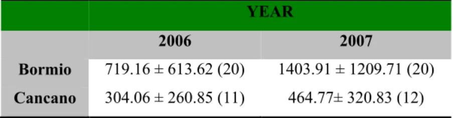
Overall, seed production in BOR was about three times higher than in CAN (site effect F1, 30 = 10.6; p = 0.003) and more seed-energy was available to squirrels in 2007 than in 2006 (year effect F1, 29 = 4.23; p = 0.049; Table 1).
Although the site*year interaction was not significant (F1, 29 = 1.62; p = 0.21), pairwise comparisons using the differences of least squares means showed that there was no significant difference between CAN and BOR in 2006 (t29 = 1.40, p = 0.17), and no significant year effect in CAN (t29 = 0.49, p = 0.63). In contrast, in BOR the 2007 seed-crop was double the size of the 2006 crop (t29 = 2.76, p = 0.01) and, consequently, in 2007 more seed-energy was produced in BOR than in CAN (t29 = 3.26, p = 0.003).
Variance explained by the random factor was small (1.1% of total variance; Log likelihood test: chi-square = 0.004, df = 1, p > 0.9), indicating that between plot variation was much smaller than variation between sites and years.
Table 1. Annual variation in tree seed production of both study sites, Cancano and Bormio. Data is presented in the
form of mean annual tree seed abundance (MJ ha-1) for all species combined (dwarf mountain pine, arolla pine, larch and norway spruce) ± SD (n).
YEAR
2006 2007
Bormio 719.16 ± 613.62 (20) 1403.91 ± 1209.71 (20)
Cancano 304.06 ± 260.85 (11) 464.77± 320.83 (12)
3.2. Squirrel Population Densities
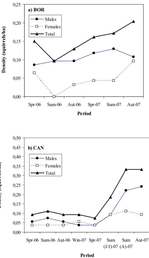
Squirrel densities were similar at BOR and CAN in 2006 (means 0.13 and 0.10 squirrels ha-1, respectively) and 2007 (means 0.20 and 0.18 squirrels ha-1, respectively; site effect F1, 12 = 0.05, p = 0.83). Between year fluctuations were more pronounced at CAN (Figure 7).
a) BOR 0,00 0,05 0,10 0,15 0,20 0,25
Spr-06 Sum-06 Aut-06 Spr-07 Sum-07 Aut-07
Period D en si ty ( sq u ir re ls /h a ) Males Females Total b) CAN 0,00 0,05 0,10 0,15 0,20 0,25 0,30 0,35 0,40 0,45 0,50
Spr-06 Sum-06 Aut-06 Win-07 Spr-07 Sum
(J/J)-07 Sum (A)-07 Aut-07 Period D en si ty ( sq u ir re ls /h a ) Males Females Total
Figure 7. Density (squirrels/ha) fluctuations of red squirrels (males, females and total densities) in both study sites,
At BOR, squirrel numbers decreased from spring to summer 2006, followed by a continuous increase from autumn 2006 until autumm 2007 (Figure 7a). At CAN, squirrel numbers were relatively stable from spring 2006 till spring of the next year, after which density increased 3-times, finally stabelising in late summer - autumn 2007 (Figure 7b). This strong increase is probably partly explained by a high trapping success of juvenile squirrels.
Summer and autumn densities tended to increase with tree seed productivity of the same year.
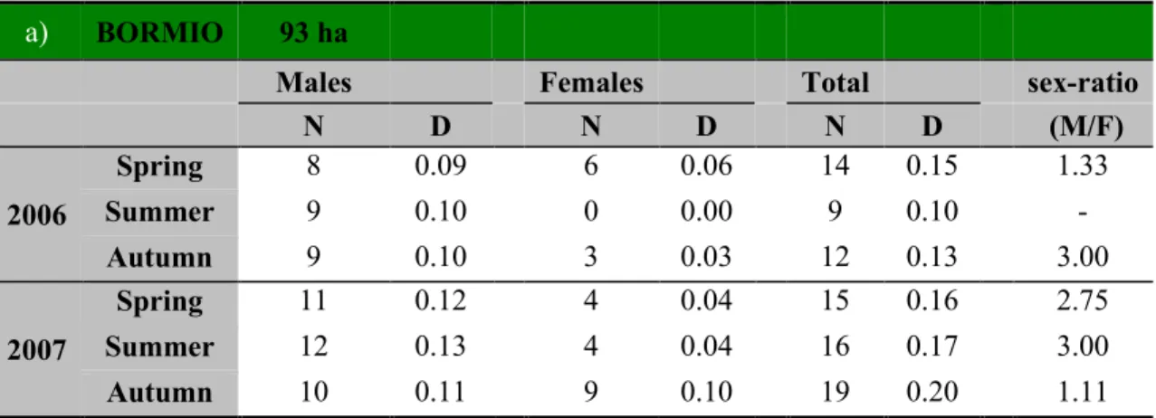
Table 2. Annual and seasonal fluctuations of red squirrels density and sex-ratio in Bormio (a) and Cancano (b) study
sites (N = number of squirrels, D = density/ha).
a) BORMIO 93 ha
Males Females Total sex-ratio
N D N D N D (M/F) 2006 Spring 8 0.09 6 0.06 14 0.15 1.33 Summer 9 0.10 0 0.00 9 0.10 - Autumn 9 0.10 3 0.03 12 0.13 3.00 2007 Spring 11 0.12 4 0.04 15 0.16 2.75 Summer 12 0.13 4 0.04 16 0.17 3.00 Autumn 10 0.11 9 0.10 19 0.20 1.11 b) CANCANO 54 ha
Males Females Total sex-ratio
N D N D N D (M/F) 2006 Spring 3 0.06 2 0.04 5 0.09 1.50 Summer 4 0.07 2 0.04 6 0.11 2.00 Autumn 3 0.06 2 0.04 5 0.09 1.50 2007 Winter 2 0.04 3 0.06 5 0.09 0.67 Spring 2 0.04 2 0.04 4 0.07 1.00
Summer (Jun / Jul) 5 0.09 5 0.09 10 0.18 1.00
Total spring (pre-breeding) densities varied little from 0.15 to 0.16 squirrels ha-1 at BOR and from 0.07 to 0.09 squirrels ha-1 at CAN. Summer densities ranged more widely from 0.10 to 0.17 squirrels ha-1 at BOR and from 0.11 to 0.33 squirrels ha-1 at CAN. Peak autumn (post-breeding) densities fluctuated between 0.13 and 0.20 squirrels ha-1 at BOR and between 0.09 and 0.33 squirrels ha-1 at CAN (Table 2). Thus, numbers typically increased at the end of spring and in autumn as a result of seasonal reproduction and immigration.
3.2.1. Female reproduction
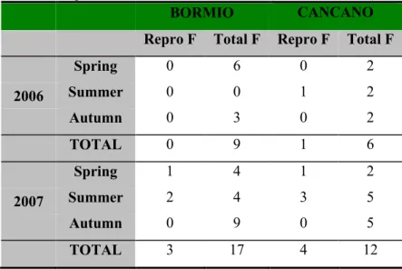
There was no successful reproduction in BOR in 2006 and only 1 female with a litter was detected in CAN in the same year (Table 3). In 2007, overall 4 reproductive events were detected on 12 cases (sum of adult females present in three periods: spring, summer and autumn) at CAN and 3 on 17 at BOR (Table 3).
Comparing proportion of litters on all females, over the three periods, showed there was no significant difference between sites (Fisher Exact test, p = 0.40).
Table 3. Annual and seasonal fluctuations of the number of reproductive female red squirrels in Bormio and Cancano
study sites (Repro F = Number of reproductive females, Total F = Number of total females).
BORMIO CANCANO
Repro F Total F Repro F Total F
Spring 0 6 0 2 2006 Summer 0 0 1 2 Autumn 0 3 0 2 TOTAL 0 9 1 6 Spring 1 4 1 2 2007 Summer 2 4 3 5 Autumn 0 9 0 5 TOTAL 3 17 4 12
3.3. Body Size and Body Mass Analysis
Between April 2006 and October 2007, 114 measurements of foot length and body mass were taken of 66 different squirrels. Individuals were captured 1 to 8 times.
The age-effect on size (foot length) did not differ among the sexes or between sites (interactions with age, all p > 0.5). Juveniles (n = 19, 56.2 ± 1.4 mm, range 52-58 mm) were smaller than subadults and adults (Figure 8a), independent of site (n = 93, 57.4 ± 1.2 mm, range 53-60 mm; age-effect F1, 108 = 18.4, p < 0.0001; site-effect F1, 108 = 1.07, p = 0.30), and, over all age-classes, males were larger than females (sex-effect F1, 108 = 4.28, p = 0.04; Figure 8a).
Juveniles weighed less than subadults and adults (juveniles n = 19, 216 ± 38 g, range 100-260 g; subadults and adults n = 93, 302 ± 28 g, range 220-380 g; Figure 8b), independent of sex and site (interactions with age, all p > 0.2). The age-effect was highly significant (F1, 107 = 117.0, p < 0.0001). Moreover, females were heavier than males (F1, 107 = 10.2, p = 0.002; Figure 8b) and squirrels from CAN were heavier than those from BOR (F1, 107 = 6.69, p = 0.011). Body mass also increased with foot length (F1, 107 = 14.7, p = 0.0002).
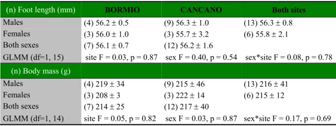
Among juveniles, foot length and body mass did not differ between sites or between the sexes (Table 4), and juvenile body mass was not affected by foot length (F1, 14 = 0.18, p = 0.68).
Table 4. Average (± SD) foot length and body mass of juvenile red squirrels (n = 19) per sex and study site. GLMM
(generalised linear mixed model) exploring effects of site, sex and sex by site on variation in foot length and body mass.
(n) Foot length (mm) BORMIO CANCANO Both sites
Males (4) 56.2 ± 0.5 (9) 56.3 ± 1.0 (13) 56.3 ± 0.8 Females (3) 56.0 ± 1.0 (3) 55.7 ± 3.2 (6) 55.8 ± 2.1 Both sexes (7) 56.1 ± 0.7 (12) 56.2 ± 1.6
GLMM (df=1, 15) site F = 0.03, p = 0.87 sex F = 0.40, p = 0.54 sex*site F = 0.08, p = 0.78
(n) Body mass (g)
Males (4) 219 ± 34 (9) 215 ± 46 (13) 216 ± 41 Females (3) 208 ± 3 (3) 222 ± 14 (6) 215 ± 12 Both sexes (7) 214 ± 25 (12) 217 ± 40
56,3 56,2 55,7 56 57,9 57,5 57,3 57 54 55 56 57 58 59 60 BOR CAN Site F o o t le n g th ( m m ) Juvenile males Juvenile females Subadult and adult males
Subadult and adult females 208 215 219 222 307 291 326 304 0 50 100 150 200 250 300 350 400 BOR CAN Site B o d y m a ss ( g ) Juvenile males Juvenile females Subadult and adult males
Subadult and adult females
a)
3.3.1. Variation in foot length of subadult and adult squirrels
Variation in foot length among subadult and adult squirrels was analysed with a stepwise backward linear mixed model exploring the effects of site, sex, year, fur colour and reproductive condition, and interactions of sex with site and with reproductive condition. None of the interaction terms were significant (all p > 0.9), and foot length did not differ with reproductive condition (F2, 85 = 0.06, p = 0.94) or fur colour (F2, 87 = 0.57, p = 0.56). There were no effects of year (F1, 89 = 0.69, p = 0.41) or site (F1, 90 = 1.50, p = 0.22; Table 5). However, foot length of males was on average 0.5 mm larger than of females (F1, 90 = 4.07, p = 0.047; Table 5).
Table 5. GLMM investigating effects of study site, sex, year, fur colour, reproductive status and interactions on
variation in foot length of subadult and adult red squirrels of both sexes, using 93 observations of 46 individuals.
Fixed effects and interactions Statistics
Sex x reproductive status F2, 82 = 0.05, p = 0.95
Sex x study site F1, 84 = 0.00, p = 0.96
Study site F1, 90 = 1.50, p = 0.22
Sex F1, 90 = 4.07, p = 0.047 Year F1, 89 = 0.69, p = 0.41
Fur-colour F2, 87 = 0.57, p = 0.56
Reproductive condition F2, 85 = 0.06, p = 0.94
3.3.2. Variation in body mass of subadult and adult squirrels
Effects of sex, site, season, year, fur colour and reproductive condition were examined as factors, and the sex by site, and sex by reproductive condition interactions on variation in body mass, using foot length as a covariate (Table 6a). Since there was a significant sex effect, females being on average heavier than males (F1, 78 = 19.8, p < 0.0001) and interaction of sex by reproductive condition (F2, 78 = 4.35, p = 0.02), the sexes were analysed separately.
On average, body mass of male squirrels increased by 14.4 (±2.28) g with each mm increase of foot length. Males were on average 16 g heavier in CAN than in BOR, but this difference was statistically not significant (partial p = 0.08; Table 6b). None of the other factors
(304.3 ± 8.1 g, differences of least squares means p = 0.004) and than anoestrus females (303.6 ± 7.1 g, DLSM p = 0.002). The latter two groups did not differ in average body mass (DLSM p = 0.95).
Table 6. GLMM investigating effects of study site, sex, year, month, fur colour, reproductive condition, interactions
and foot length as co-variate on variation in body mass of subadult and adult red squirrels: a) both sexes, using 93 observations of 46 individuals, b) males, using 62 observations of 26 individuals, and c) females, using 31 observations of 20 individuals. aExcluded from the model.
Fixed effects and interactions Statistics (a) Sexes pooled
Sex x reproductive status F2, 78 = 4.35, p = 0.02 Sex x study site F1, 78 = 0.02, p = 0.88
Foot length F1, 78 = 29.2, p < 0.0001 Study site F1, 78 = 0.39, p = 0.53 Sex F1, 78 = 19.8, p < 0.0001 Month F3, 78 = 0.93, p = 0.43 Year F1, 78 = 5.42, p = 0.02 Fur-colour F2, 78 = 3.24, p = 0.045 Reproductive condition F2, 78 = 1.79, p = 0.17 (b) Males Foot length F1, 59 = 37.0, p < 0.0001 Study site F1, 59 = 3.17, p = 0.08 Month F3, 51 = 0.10, p = 0.96 a Year F1, 58 = 2.58, p = 0.11 a Fur-colour F2, 56 = 2.31, p = 0.11 a Reproductive condition F2, 54 = 0.14, p = 0.87 a (c) Females Foot length F1, 27 = 2.74, p = 0.11 a Study site F1, 26 = 0.25, p = 0.62 a Month F3, 23 = 1.61, p = 0.22 a Year F1, 22 = 0.87, p = 0.36 a Fur-colour F1, 21 = 0.66, p = 0.42 a Reproductive condition F2, 28 = 6.66, p = 0.004
3.4. Space Use Analysis
In a preliminary test, it was explored whether home ranges at CAN differed between 2006 and 2007. Since there was no significant year effect (ln MCP, F1, 16 = 0.40, p = 0.54; ln KDE95%, F1, 16 = 0.00, p = 0.97; ln KDE85%, F1, 16 = 1.21, p = 0.29), data were pooled over both years for further comparisons with space use at BOR (where data were only available for 2007).
a) spring-summer 4,71 32,86 9,39 5,47 0 10 20 30 40 50 60 BOR CAN S iz e (h a ) b) autumn 16,53 8,82 11,15 10,78 0 5 10 15 20 25 BOR CAN MALE FEMALE a) spring-summer 7,59 7,43 64,65 15,1 0 20 40 60 80 100 BOR CAN S iz e (h a ) b) autumn 32,08 11,68 17,02 11,9 0 10 20 30 40 50 BOR CAN a) spring-summer 7,59 7,43 57,23 13,96 20 40 60 80 100 S iz e (h a ) b) autumn 29,56 11,68 16,38 11,9 10 20 30 40 50 9.1) MCP 9.2) KDE 95% 9.3) KDE 85%
In the GLMM with ln MCP, ln KDE 95% and ln KDE 85% of home range size as dependent variables, the effects of sex, site, season, foot length, number of nuclei and number of fixes were examined as factors, and the sex by site, sex by season and season by site interactions.
Using ln MCP of home range size as dependent variable, there was a significant site effect, with ranges at CAN being on average bigger than those of BOR (F1, 27 = 14.08, p = 0.0009) and a significant sex by site interaction (F1, 27 = 6.04, p = 0.02; Table 7a). None of the other factors were significant (Table 7a).
Male red squirrels had larger ranges at CAN than at BOR (t28 = 4.37, p = 0.0002; Figure 9.1). At CAN, males used larger ranges than females (t28 = 2.97, p = 0.006), but this was not the case at BOR (t28 = -0.42, p = 0.68; Figure 9.1). There was no significant difference between sites among female squirrels (t28 = 0.76, p = 0.45).
Using ln KDE 95% of home range size as dependent variable, there was a significant site effect, with ranges at CAN being on average bigger than those of BOR (F1, 26 = 48.47, p < 0.0001) and a significant sex effect, with male ranges being on average bigger than those of females (F1, 26 = 13.17, p = 0.001; Table 7b). There was also a significant sex by site interaction (F1, 26 = 13.15, p = 0.001) and season by site interaction (F1, 26 = 6.06, p = 0.02; Table 7b).
Ranges were larger at CAN than at BOR for males (t26 = 8.22, p < 0.0001) and females (t26 = 2.19, p = 0.04; Figure 9.2). At CAN, males used larger ranges than females (t26 = 5.60, p < 0.0001), but this was not the case at BOR (t26 = 0.00, p = 0.99). Both in spring-summer (t26 = 7.01, p < 0.0001) and in autumn (t26 = 3.12, p = 0.004), ranges were larger at CAN than at BOR (Figure 9.2). At CAN, there was no difference between spring-summer and autumn ranges (t26 = 1.41, p = 0.17), whereas at BOR spring-summer ranges tended to be smaller than autumn ranges, without being significant (t26 = -2.04, p = 0.052).
Using ln KDE 85% of home range size as dependent variable, there was a significant site effect, with larger core areas at CAN than BOR (F1, 28 = 29.7, p < 0.0001) and males had larger core areas than females (sex-effect: F1, 28 = 9.83, p = 0.004; Table 7c). There was also a significant sex by site interaction (F1, 28 = 9.13, p = 0.005; Table 7c).
Core areas were larger at CAN than BOR for males (t28 = 6.56, p < 0.0001), but not for females (t28 = 1.59, p = 0.12; Figure 9.3). At CAN males had larger core areas than females (t28 = 4.77, p < 0.0001) but core areas did not differ between the sexes at BOR (t28 = 0.08, p = 0.94).
Table 7. GLMM investigating effects of study site, sex, season, number of nuclei, footlength, number of fixes and
interactions on variation in home range size of red squirrels (18 males and 14 females), according to: a) MCP, b) KDE 95% and c) KDE 85% methods.
Fixed effects and interactions Statistics (a) MCP
Study site F1, 27 = 14.08, p = 0.0009
Sex F1, 27 = 3.44, p = 0.07
Study site x sex F1, 27 = 6.04, p = 0.02 Season F1, 26 = 0.41, p = 0.53
Study site x season F1, 25 = 3.36, p = 0.08
Sex x season F1, 21 = 1.94, p = 0.18 Nuclei F2, 22 = 0.51, p = 0.61 Footlength F1, 24 = 1.65, p = 0.21 Fix F1, 27 = 4.19, p = 0.0504 (b) KDE 95% Study site F1, 26 = 48.47, p < 0.0001 Sex F1, 26 = 13.17, p = 0.001 Study site x sex F1, 26 = 13.15, p = 0.001 Season F1, 26 = 0.36, p = 0.55
Study site x season F1, 26 = 6.06, p = 0.02 Sex x season F1, 21 = 2.25, p = 0.15 Nuclei F2, 23 = 0.31, p = 0.73 Footlength F1, 22 = 0.08, p = 0.78 Fix F1, 25 = 0.06, p = 0.81 (c) KDE 85% Study site F1, 28 = 29.65, p < 0.0001 Sex F1, 28 = 9.83, p = 0.004 Study site x sex F1, 28 = 9.13, p = 0.005 Season F1, 27 = 0.21, p = 0.65
Study site x season F1, 26 = 3.76, p = 0.06
Sex x season F1, 21 = 1.44, p = 0.24
Nuclei F2, 23 = 0.36, p = 0.70
Footlength F1, 22 = 0.02, p = 0.89
3.4.1. Core area overlap
Variance explained by the random factor was 14% of total variance (Log likelihood test: chi-square = 2.75, df = 1, p < 0.05), indicating there was a significant amount of individual variation in core-area overlap patterns.
101,80 38,94 18,20 36,28 0 20 40 60 80 100 120 140 160 180 MALE FEMALE Sex M ea n c o re a re a o v er la p MALE OVERLAP FEMALE OVERLAP
Figure 10. Mean core area overlap (+ 1 SD) of male (n = 18) and female (n = 14) red squirrels by core areas of both
sexes in both study sites, Bormio and Cancano.
In a GLMM with sex and overlapping sex as factors, and the sex by overlapping sex interaction, there was a significant effect of sex overlapping (F1, 47 = 21.49, p < 0.0001) and sex by sex overlapping interaction (F1, 47 = 18.91, p < 0.0001) on variation in red squirrels core area overlap (Table 8a).
Males were overlapped to same extent by other males and by females (t47 = 0.21, p = 0.83; Figure 10). Females were overlapped more by males than by other females (t47 = 6.08, p < 0.0001; Figure 10). There was no difference between male-male and female-female overlap (t47 = 1.55, p = 0.13), but females were overlapped to a higher extent by males than males by other males (t47 = -3.92, p = 0.0003), suggesting that males concentrated their space use near female core areas (Figure 10). Intra-sexual overlap among females was the lowest of all sex by sex combinations and not significantly different from 0 (least squares means 14 ± 11% t-test mean different from 0: t47 = 1.27, p = 0.21).
Since there was a significant sex by sex overlap interaction, the effects of site, season and site by season on variation in red squirrels core area overlap were analysed separately, on all the
There were no significant effects found on the combinations males by males and males by females (Table 8b and c).
On the combination females by males, there was a significant site effect (F1, 6 = 18.6, p = 0.005; Table 8d). Females were overlapped more by males at CAN than at BOR (t6 = 4.31, p = 0.005) and there was a non-significant tendency for higher overlap in spring-summer when mating takes place (unpublished data) than in autumn (t3 = 3.02, p = 0.06). The season effect was significant only at CAN (t3 = 4.64, p = 0.02) and the site effect was only significant in spring-summer due to very high overlap in spring-spring-summer at CAN (t3 = 4.97, p = 0.02).
There were no significant effects found on the combination females by females (Table 8e). There is some degree of core-area overlap among females at CAN (t-test mean different from 0: t6 = 2.88, p = 0.03), but at BOR females used exclusive core areas not shared by other females (t-test mean different from 0: t6 = 0.00, p = 1.00).
Table 8. GLMM investigating effects of sex, sex overlap and sex by sex overlap on variation in red squirrels core area
overlap (18 males and 14 females) (a). GLMM investigating effects of site, season and site by season on variation in red squirrels core area overlap: b) males by males, c) males by females, d) females by males, e) females by females.
Fixed effects and interactions Statistics (a)
Sex F1, 47 = 2.57, p = 0.12
Sex overlap F1, 47 = 21.49, p < 0.0001 Sex x sex overlap F1, 47 = 18.91, p < 0.0001
(b) Males by males
Study site F1, 7 = 0.96, p = 0.36
Season F1, 5 = 5.73, p = 0.06
Study site x season F1, 5 = 0.96, p = 0.37
(c) Males by females
Study site F1, 7 = 0.00, p = 0.97
Season F1, 5 = 0.96, p = 0.37
Study site x season F1, 5 = 0.14, p = 0.73
(d) Females by males
Study site F1, 6 = 18.62, p = 0.005 Season F1, 3 = 9.12, p = 0.06
3.4.2. Site fidelity
Average site fidelity was high in both study areas (78 ± 7% at CAN and 72 ± 7% at BOR). Average site fidelity did not differ between the sites (F1, 5 = 0.02, p = 0.88) or between the sexes (F1, 6 = 1.64, p = 0.25; Table 10). There were no effects on site fidelity for any of the variables that were explored in the GLM model (Table 10).
Table 10. GLMM investigating effects of study site, sex, reproductive condition, body mass, footlength and
interactions on variation in site fidelity of red squirrel core areas (n = 6 at Bormio and 8 at Cancano).
Fixed effects and interactions Statistics
Study site F1, 5 = 0.02, p = 0.88
Sex F1, 6 = 1.64, p = 0.25
Study site x sex F2, 7 = 0.89, p = 0.45
Reproductive condition F1, 9 = 0.10, p = 0.75
Sex x reproductive condition F1, 10 = 0.17, p = 0.69
Body mass F1, 11 = 0.43, p = 0.53
4. Discussion
4.1. Variation in seed availability
In 2006, seed-energy available to red squirrels did not differ between the study sites, but in 2007 considerably more energy was produced in BOR than in CAN (1403.91 ± 1209.71 MJ ha-1 and 464.77 ± 320.83 MJ ha-1, respectively). Therefore, the first prediction, that seed-crop size would be smaller and hence food resources would be more limited in CAN, was confirmed only in 2007. This difference was expected since CAN has only a single major food resource, dwarf mountain pine seeds, with a mean energy-content of 5.7 kJ per cone, while in BOR the dominant tree species, Arolla pine, is interspersed with isolated Norway spruce and larch trees. All these species have a higher mean energy-content per cone (121.3 kJ for Arolla pine, 51.0 kJ for Norway spruce and 9.4 kJ for larch). Moreover, in 2006 Arolla pine produced no or few cones per tree (on average 4), while in 2007 there was a medium-good seed-crop (23 cones/tree). Thus, these 2-year data suggest that food abundance in CAN is similar to BOR when Arolla pine produces a poor seed-crop and there is no masting of Norway spruce, while medium to good seed production by Arolla pine results in higher food abundance in BOR than CAN. So, BOR probably "behaves" as a marginal habitat (a sink) in years with poor pine-crops, but as a medium-quality habitat in years of good pine-crops.To date, seed-crop monitoring in CAN was too short to explore the existence of masting, a high and synchronised, episodic seed production (Smith 1970, Silvertown 1980), in this species.
Seed productivity in both study sites was higher than man-made conifer forests in northern England (26-36 MJ ha-1, Lurz et al. 1995, 2000; Wauters et al. 2000) but significantly lower than coniferous woodlands dominated by Scots pine (Pinus sylvestris) and/or Corsican pine (Pinus
nigra) in southern England and Belgium (500-5600 MJ ha-1, Wauters & Lens 1995; Kenward et al.
1998) and mixed deciduous woodlands and mixed woodlands dominated by oak (Quercus robur), beech (Fagus sylvatica) and Scots pine in southern England, Belgium and North Italy (2500-20