A MULTICRITERIA PRIORITIZATION MODEL TO SUPPORT PUBLIC SAFETY PLANNING
Andr´e Morais Gurgel
1and Caroline Maria de Miranda Mota
2*Received October 26, 2011 / Accepted January 23, 2013
ABSTRACT.Setting out to solve operational problems is a frequent part of decision making on public safety. However, the pillars of tactics and strategy are normally disregarded. Thus, this paper focuses on a strategic issue, namely that of a city prioritizing areasin which there is a degree of occurrences for crim-inality to increase. A multiple criteria approach is taken. The reason for this is that such a situation is normally analyzed from the perspective of the degree of police occurrences. The proposed model is based on a SMARTS multicriteria method and was applied in a Brazilian City. It combines a multicriteria method and a Monte Carlo Simulation to support an analysis of robustness. As a result, we highlight some dif-ferences between the model developed and police occurrences model. It might support differentiated poli-cies for zones, by indicating where there should be strong actions, infrastructure investments, monitoring procedures and others public safety policies.
Keywords: public safety, prioritization, SMARTS.
1 INTRODUCTION
The World Health Organization defines violence as the intentional use of physical force against oneself, a person or a community. As a result, Kruget al.(2002) divided it into three sets which they called: collective, self-directed or interpersonal violence which is characterized mainly as urban violence.
Therefore, the strong combat of crime and public policies such as bringing about long-term improvements in income and in education and reducing unemployment are requirements if urban violence is to be reduced. However, there is a resources shortage that prevents the simultaneous application of such actions in the same proportions in all areas in a city.
*Corresponding author
1Federal University of Pernambuco, Brazil. PhD Student at Postgraduate Program in Production Engineering from Federal University of Pernambuco. E-mail: [email protected]
Consequently, several studies tackled police operational problems as scheduling problems (Tay-lor & Huxley, 1989; Zenget al., 2006), as facility location problems (D’Amico, 2002; Curtinet al., 2007) and as econometric models (Correa, 2005; Wanget al., 2005; Yusufet al., 2011).
These models could contribute towards reducing operational costs, although it is also important that public safety decision makers receive support with regard to strategic and tactical issues that would allow effective public policies to develop.
As a result, a strategic model was drawn up to support the decision maker in evaluating the differ-ences between zones in a city from a multicriteria perspective, whereas hit her to the perspective of the degree of police occurrences has normally been used to analyze these differences.
This paper sets out a multicriteria model that seeks to prioritize areas based on spatial criminol-ogy using social and demographic criteria. It will allow points of danger to be visualized that need different actions such as investment in the infrastructure. In addition, it permits different policies for safe places, such as monitoring policies being more necessary than other policies.
This paper is structured into six sections: Section 1 contextualizes the problem of violence and defines the problem; Section 2 gives an overview of spatial criminology; Section 3 reviews SMARTS and SMARTER methods; Section 4 gives a detailed presentation of the problem; in Section 5 there is a numerical application and Section 6 draws some conclusions and gives some final remarks.
2 SPATIAL CRIMINOLOGY
According to Townsley (2009), criminology is the study of criminals, their actions (crimes), and society’s response to these actions (the criminal justice system). Thus, Andresen (2011) defines spatial criminology as a sub-field that seeks to understand the variation of criminal activity across the urban landscape. The use that some published papers have made of these concepts is given below.
Andresen (2011) developed a statistical model to identify local crime clusters. A tool that he used for his problem was a sub-field within geographic information science called local indicators of spatial association (LISA) and he defined social indices as explanatory variables. Therefore, his model was able to identify some patterns for specific crime types in Vancouver City.
Yang (2009) designed an experiment to disprove the broken windows thesis that neighborhood disorder is the root of violent crime. He uses spatial analysis to correlate hot spots of violent crime and disorder. Thus, he showed that places that are free of disorder are guaranteed to have low rates of violence. However, high levels of disorder were not predictors of problems of violence.
Stucky & Ottensmann (2009) proposed a statistical model to identify some crime patterns on land use in a region. Thus, they divided land use into categories such as business premises, hospitals, schools and churches. Moreover, they included socio-economic characteristics and correlated these to crime rates. They looked for a pattern to the structure of land use that would indicate the prevalence of certain types of crime. Their findings were that some forms of commercial activity and high-density residential lands were associated with high criminality.
In addition, there are theoretical approaches such as that taken by Townsley (2009) which studies the importance of geography for criminology studies and focuses on new advances. He draws attention to spatial autocorrelation. Furthermore, Tita & Radil (2010) discuss new challenges on spatial analysis focusing mainly on the concept of “place”.
3 SMARTS
A multicriteria decision refers to situations in which there areat least two alternative actions to choose from. Thus, Roy (1996) defines decision support as an activity that enables the problem to be clarified by supporting a decision maker to find a solution that is compatible with his/her preference structure.
Given that that there is a large number of contexts, a multicriteria model has often been applied to situations, such as: portfolio problems (Almeida & Duarte, 2011; Ballestero et al., 2012; Ehrgottet al., 2012), water supply (Moraiset al., 2010; Abu-Taleb & Mareschal, 1995), selecting members of a project team (Alencar & Almeida, 2010), building inventory (Szajubok et al., 2006), preventive maintenance (Chareonsuket al., 1997; Cavalcanteet al., 2010), information systems planning (Almeida Filho & Cabral, 2010) and so forth.
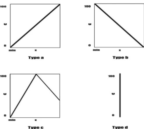
According to Edwards & Barron (1994), SMARTS is a modification of the SMART method which used an additive model, given that the latter considered the importance of criteria. This correction was necessary, since additive methods use an interval scale. Moreover, SMARTS is an additive single criterion synthesis method. Hence, it aggregates all criteria on a single criterion synthesis using a compensatory logic as shown in Equation 1.
Vh= N X
n=1
kn·vh(xhn) (1)
where:
Kn: criterion scale constantn;
vh(xhn): function value to criterionnfor each alternativeh;
N: number of criteria.
Figure 1– One-dimensional utility functions applied to SMARTS. Source: Edwards & Barron (1994).
Moreover, Edwards & Barron (1994) developed another method named SMARTER that is char-acterized by its use of preference ranking to obtain Rank Order Centroid (ROC) weight criteria without applying a second phase from swing weights. Thus, it is important to analyze the prob-lem and the decision maker’s characteristics so as to choose the best method for each model.
Choosing a proper multicriteria method is an important aspect of the decision process. The model should provide a ranking of actions, more precisely, the prioritization of zones of a city in order to support public safety policies. Thus, we selected the SMARTS method, since that it is easy to use, if correctly applied, and enables the decision maker to solve a ranking problem. As the method is classified as an additive method, it reflects a compensatory effect which must be accepted by the decision maker.
Besides the simplicity of SMARTS, it requires a careful elicitation process of the constants of scales in order to reflect the trade-off amongst the criteria (Keeney & Raiffa, 1976; Daher & Almeida, 2012). Hence, we propose to reduce this effort by a swing weights elicitation proce-dure combined with a Monte Carlo Simulation that analyze the results of the model. Using this approach, the preferences of the decision maker is still taken into account.
4 MULTICRITERIA MODEL FOR PRIORITIZING URBAN AREAS FOCUSING ON
FACTORS THAT CAN AFFECT URBAN CRIMINALITY
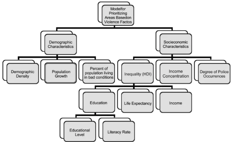
Thus, the multi-criteria model, which was structured on factors that influence criminality, in-volves mainly socioeconomic and demographic issues as indicated by Coulton & Pandey (1992) and Andresen (2011). From this reasoning, a criteria hierarchy emerges as demonstrated in Figure 2.
Figure 2– Model for prioritizing regions based on factors of violence.
These criteria were collected in various ways, as detailed in the list:
• Population density: defined as people/km2. It is a representative criterion as shown in Stucky & Ostelman (2009);
• Population growth: the percentage growth in population between one census and another. Andresen (2011) showed the importance of this criterion in his paper;
• Percentage of population living in bad conditions: percentage of people living in unfit housing or sites with deficient infrastructure;
• HDI: measures the degree of inequality. It is used in a qualitative scale defined by the Human Development Report in 2010 which divides the regions into four distinct classes;
• Income concentration: this uses the GINI index to measure the income concentration on a scale of 0 to 1, where 1 means maximum inequality;
• Degree of police occurrences: a qualitative criterion that varies between 1 and 5 and meas-ures the level of events occurring in each zone.
According to Klugmanet al. (2011), HDI is a composite index aggregating three basic dimen-sions into a summary measurement using country level information. It is noteworthy that the HDI is formed from statistics on health, education and living standards dimensions that are ag-gregated according to the Human Development Report (HDR), using an additive value function that varies between 0 and 1 as shown in Eq. 2:
H D I = Hh+He+Hls
3
Hh=
le−lemin lemax−lemin
He =
1 3 ·
ger−germin germax−germin
+2/3·
li t−li tmin li tmax−li tmin
Hls =
ln(gd p)−ln(gd pmin)) ln(gd pmax)−ln(gd pmin)
(2)
where: Hh: health;
He: education;
Hls: dimensions of living standards;
le: life expectancy; ger: gross enrolment ratio; li t: literacy;
gd p: GDP per capita.
According to Klugmanet al.(2011), this indicator received some critiques such as the choice of variables excludes some dimensions, such as equity, sustainability and happiness. Moreover, it has a functional form that causes some concern, such as its normalization of indicators.
Thus, the HDI was reformulated in 2010 and incorporated improvements such as a geometric mean and new sub criteria as shown in Eq. 3.
H D I =(Hh·He·Hls)1/3
Hh=
le−lemin lemax−lemin
He=
mys−mysmin mysmax−mysmin
·
eys−eysmin eysmax−eysmin
1/2
Hls =
ln(gni)−ln(gnimin) ln(gnimax)−ln(gnimin)
(3)
where: Hh: health;
He: education;
le: life expectancy;
mys: mean years of schooling; eys: expected years of schooling; gni: gross national income.
These modifications ended some HDI problems, mainly on the method of aggregation. Thus, it is a useful estimate for measuring the inequality difference across countries.
Income concentration is a dimension characterized as being calculated by an index, viz. the Gini coefficient. According to Jedrzejczak (2008), the Gini index can be used to measure the spread of a distribution of income, consumption, or wealth and can be expressed as a ratio of two regions defined by a line of equal shares and a Lorenz curve in a unit box, such as Lorenz (1905) developed in his paper.
Therefore, by using these concepts, it is possible to compare different areas and determine a measurement scale of between 0 and 1, 0 being an equality region and 1 an income zone of complete inequality. Thus, in this case a maximization functional form was established, given that higher indices generate a greater degree of occurrences to a growth in violence.
Finally, degrees of police occurrences are measured on a qualitative scale. Thus, the decision maker defines a degree of criminality based on his/her knowledge of the violence in each area.
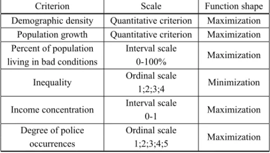
Subsequently, it is possible to formulate a final aggregation function for this model and a brief summary of the criteria structure from the model, as shown in Table 1 and Eq. 4.
Table 1– Summary of criteria structure.
Criterion Scale Function shape
Demographic density Quantitative criterion Maximization Population growth Quantitative criterion Maximization Percent of population Interval scale
Maximization living in bad conditions 0-100%
Inequality Ordinal scale Minimization
1;2;3;4
Income concentration Interval scale Maximization 0-1
Degree of police Ordinal scale
Maximization
occurrences 1;2;3;4;5
Vh=
6
X
n=1
kn·vh(xhn) (4)
where:
h: alternativeh;
kn:ncriterion scale constant;
vh(xhn):ncriterion function value to alternativeh.
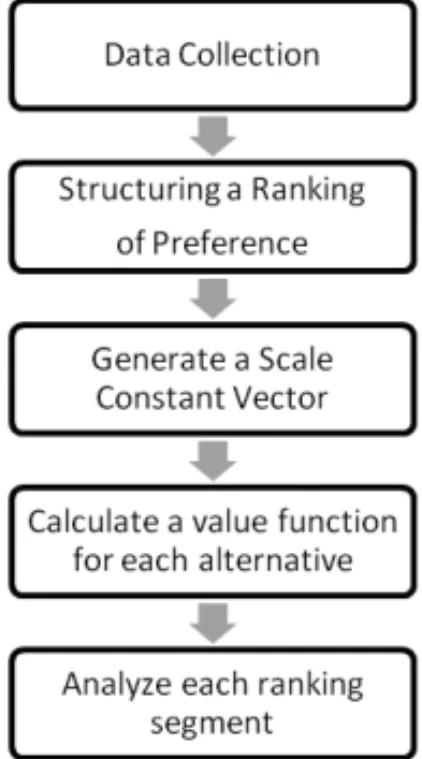
Therefore, a framework was formulated so as to apply the model in a consistent manner, as shown in Figure 3.
Figure 3– Model framework.
5 NUMERICAL APPLICATION
Usually in criminality analysis, the number or the degree of occurrences in each region/zone is noted. However, it is important to aggregate other factors to increase the accuracy of the analysis of violence, as shown in Section 4.
The model was applied in the City of Recife. The city was divided into 62 human development units, as per the 2000 UDR, as shown in Appendix. The data were collected from the 2006 Human Development Atlas of Recife. However, the degree of occurrences data was aggregated based in the number of occurrences. Thus, we used the decision maker’s knowledge and these events to create a scale going from a very low to a very high degree of occurrences for the growth in criminality.
Based on this degree of occurrences, it was divided the zones into five subsets, as enumerated below.
Very low degree of occurrences:
{A2, A3, A7, A16, A17, A26, A29, A36, A40, A51, A61}
Low degree of occurrences:
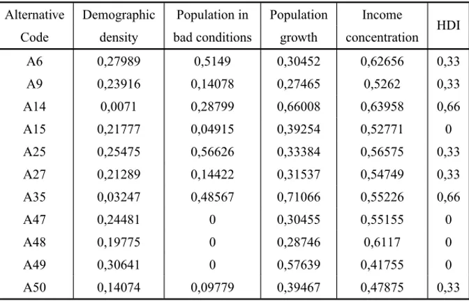
{A6, A9, A14, A15, A25, A27, A35, A47, A48, A49, A50}
Medium degree of occurrences:
High degree of occurrences:
{A8, A12, A13, A21, A24, A30, A31, A34, A44, A46, A56, A57, A58, A59}
Very high degree of occurrences:
{A4, A5, A10, A11, A18, A19, A38, A41, A52, A53, A54, A62}
In addition, a first phase of “swing weights” procedure was applied to define a ranking of prefer-ences for the set of criteria, as shown in Table 2. However, it is difficult for the decision maker in this model to define a unique scale constant vector. Moreover, it is necessary to generate constant scale vectors using this ranking preference as a guideline. Hence, considering the preferences of the decision maker, a SMARTER method was applied so that a scale constant vector was generated, as shown in Table 3.
Table 2– Decision maker’s preference structure.
Ranking Criterion
1st Demographic Density
2nd Percent of Population Living in Bad Conditions 3rd Degree of Police Occurrences
4th Inequality – Human Development Index (HDI) 5th Percent of Growth in Population
6th Income Concentration (GINI Index)
Table 3– Scale constants criteria based on smarter method.
Criterion Scale constant
Demographic density (1+1/2+1/3+1/4+1/5+1/6)
6 =0.40833
Percent of population (0+1/2+1/3+1/4+1/5+1/6)
6 =0.24167
living in bad conditions
Degree of police occurrences (0+0+1/3+1/4+1/5+1/6)
6 =0.15833
Inequality – (0+0+0+1/4+1/5+1/6)
6 =0.10278
Human Development Index (HDI)
Percent of population growth (0+0+0+0+1/5+1/6)
6 =0.06111
Income concentration (GINI Index) (0+0+0+0+0+1/6)
Therefore, the model shows a difference between police degree occurrences analysis in all five segments. As observed in Figure 4 and Figure 5, there are key changes that demonstrate model applicability.
Figure 4 – Comparison between the model of the degree of police occurrences and multicriteria prioritization from zone A1 to A31.
For example, Alternative A1 it was allocated on medium degree of occurrences to criminal-ity growth, but it on multicriteria model this alternative was positioned on first place in the SMARTER ranking.
In addition, a sensitivity analysis tests the robustness of the model by using a Monte Carlo Sim-ulation. This generates ten thousand constant scale vectors uniformly distributed and an SMAA first phase procedure developed by Tervonen & Lahdelma (2007) was applied, thus creating the sets of weight criteria, as shown on Algorithm 1.
Algorithm 1– Scale constant vec-tor generation procedure. Source: Tervonen & Lahdelma (2007).
Output:kvector 1: forj←1 to 5 do 2: qj←RANDOMU[0,1] 3: end for
4: SORTasc(q) 5: q0←0 6: q6←1
7: forj←1 to 6 do 8: kj ←qj−qj−1 9: end for
Thereafter, it is possible to calculate a global function value for each alternative using all the vectors generated by the Algorithm 1 procedure. However, it is necessary to do some robustness analyses. For this, some indicators were developed, such as those given in Eqs. 5, 6, 7 and 8.
I1= n1
N (5)
where:
n1: number of alternatives in the same position as in the SMARTER ranking; N: number of alternatives in set.
I2= n2
N (6)
where:
n2: number of alternatives between one position above or below the SMARTER ranking; N: number of alternatives in set.
I3= n3
N (7)
where:
I4= n4
N
where:
n4: number of alternatives among three positions above or below the SMARTER ranking; N: number of alternatives in set.
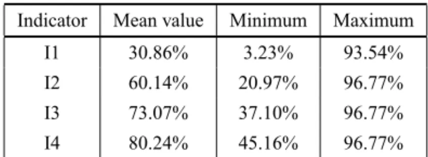
In Table 4, the I1 indicator has a low correlation as between the SMARTER ranking and the sensitivity analysis ranking. However, this happens since the variation in the scale constants is very large.
Table 4– Sensitivity analysis indicators.
Indicator Mean value Minimum Maximum
I1 30.86% 3.23% 93.54%
I2 60.14% 20.97% 96.77%
I3 73.07% 37.10% 96.77%
I4 80.24% 45.16% 96.77%
However, at I2, I3 and I4 a high correlation is observed between the SMARTER and analysis rankings. Therefore, these indicators show the model is robust, given that a large variation in scale constants does not cause a great change in ranking. In addition, when a segment analysis is conducted, there are not large changes in the subsets.
6 CONCLUDING REMARKS
Public safety planning involves three action plans, namely operational, strategic and tactical ones. Many papers have contributed to operational models, but they have not dealt with strate-gic problems. Thus, it is noted that stratestrate-gic planningfor a region is important so as to allocate differentiated public policies that support combating and reducing violence and criminality.
Hence, a multicriteria model combined with a Monte Carlo Simulation was developed to allow zone ranking based on demographic and socioeconomic issues that may have an impact on vio-lence. Moreover, this model was applied in the City of Recife to examine its soundness and this led to a robust result which allows the decision maker to transform the alternatives into subsets and for different public policies to be created for each one.
It was concluded that the model developed is applicable and can be expanded to other regions where it may help to improve the management of public safety and to reduce violence. However, it is important to note that this model is applicable to situations where the decision maker has a compensatory preference structure and is unable to elicit a single constant scale vector.
preference structure and other important criteria that incorporate new characteristics to improve this model, such as geographic conditions and the absolute number of occurrences.
REFERENCES
[1] ABU-TALEBMF & MARESCHALB. 1995. Water Resources planning in the Middle East: Applica-tion of the PROMETHEE V multicriteria method.European Journal of Operational Research,81(3): 500–511.
[2] ALENCARLH & ALMEIDAAT. 2010. A model for selecting project team members using multicri-teria group decision making.Pesquisa Operacional,30: 221–236.
[3] ALMEIDAAT & DUARTEMDO. 2011. A multi-criteria decision model for selecting project portfolio with consideration being given to a new concept for synergies.Pesquisa Operacional,31: 301–318.
[4] ALMEIDAFILHOAT & COSTAAPCS. 2010. Um modelo de otimizac¸˜ao para priorizac¸˜ao em plane-jamento de Sistemas de Informac¸˜ao.Produc¸˜ao,20: 265–273.
[5] ANDRESENMA. 2011. Estimating the probability of local crime clusters: The impact of immediate spatial neighbors.Journal of Criminal Justice,39(5): 394–404.
[6] ANDRESENMA & MALLESONN. 2010. Testing the Stability of Crime Patterns: Implications for Theory and Policy.Journal of Research in Crime and Delinquency,48(1): 58–82.
[7] BALLESTEROE, BRAVOM, P ´EREZ-GLADISHB, ARENAS-PARRA M & PLA-SANTAMARIA` D. 2012. Socially Responsible Investment: A multicriteria approach to portfolio selection combining ethical and financial objectives.European Journal of Operational Research,216(2): 487–494.
[8] CAVALCANTE CAV, FERREIRARJP & ALMEIDAAT. 2010. A preventive maintenance decision model based on multicriteria method PROMETHEE II integrated with Bayesian approach.IMA Jour-nal of Management Mathematics(Print),21: 333–348.
[9] CHAREONSUKC, NAGARURN & TABUCANONMT. 1997. A multicriteria approach to the selection of preventive maintenance intervals.International Journal of Production Economics,49(1): 55–64.
[10] COULTON CJ & PANDEYS. 1992. Geographic Concentration of Poverty and Risk to Children in Urban Neighborhoods.American Behavioral Scientist,35(3): 238–257.
[11] CORREAH. 2005. Optimal expenditures on police protection.Socio-Economic Planning Sciences, 39(3): 215–228.
[12] CURTINKM, HAYSLETT-MCCALLK & QIUF. 2007. Determining Optimal Police Patrol Areas with Maximal Covering and Backup Covering Location Models.Networks and Spatial Economics, 10(1): 125–145.
[13] D’AMICOS. 2002. A simulated annealing approach to police district design.Computers & Opera-tions Research,29(6): 667–684.
[14] DAHER SFD & ALMEIDA AT. 2012. The Use of Ranking Veto to Mitigate the Compensatory Effects of Additive Aggregation in Group Decisions on a Water Utility Automation Investment.Group Decision and Negotiation,21(2): 185–204.
[16] EHRGOTTM, KLAMROTHK & SCHWEHMC. 2004. An MCDM approach to portfolio optimization. Traffic and Transportation System Analysis,155(3): 752–770.
[17] JEDRZEJCZAK A. 2008. Decomposition of the Gini Index by Sources of Income. International Advances in Economic Research,14(4): 441–447.
[18] KEENEYR & RAIFFAH. 1976. Decisions with Multiple Objectives, Wiley.
[19] KLUGMAN J, RODR´IGUEZF & CHOIHJ. 2011. The HDI 2010: new controversies, old critiques. The Journal of Economic Inequality,9(2): 249–288.
[20] KRUGEG, DAHLBERGLL, MERCYJA, ZWIAB & LOZANOR. 2002. World Report on Violence and Health, WHO, Geneva, Swiss.
[21] LORENZMO. 1905. Methods of Measuring the Concentration of Wealth.Publications of the Ameri-can Statistical Association,9(70): 209–219.
[22] MORAISDC, CAVALCANTE CAV & ALMEIDA AT. 2010. Priorizac¸˜ao de ´Areas de Controle de Perdas em Redes de distribuic¸˜ao de ´Agua.Pesquisa Operacional,30: 15–32.
[23] ROYB. 1996. Multicriteria Methodology for Decision Aiding, Springer Verlag.
[24] STUCKYTD & OTTENSMANNJR. 2009. Land Use and Violent Crime.Criminology,47(4): 1223– 1264.
[25] SZAJUBOKNK, MOTACMM & ALMEIDAAT. 2006. Uso do M´etodo Multicrit´erio ELECTRE TRI para Classificac¸˜ao de Estoques na Construc¸˜ao Civil.Pesquisa Operacional,26: 625–648.
[26] TAYLORPE & HUXLEY SJ. 1989. A Break from Tradition for the San Francisco Police: Patrol Officer Scheduling Using an Optimization-Based Decision Support System.Interfaces,19(1): 4–24.
[27] TERVONENT & LAHDELMAR. 2007. Implementing stochastic multicriteria acceptability analysis. European Journal of Operational Research,178(2): 500–513.
[28] TITAGE & RADILSM. 2010. Making Space for Theory: The Challenges of Theorizing Space and Place for Spatial Analysis in Criminology.Journal of Quantitative Criminology,26(4): 467–479.
[29] TOWNSLEYM. 2009. Spatial Autocorrelation and Impacts on Criminology.Geographical Analysis, 41(4): 452–461.
[30] WANGSJ, BATTA R & RUMPCM. 2005. Stability of a crime level equilibrium.Socio-Economic Planning Sciences,39(3): 229–244.
[31] YANG SM. 2009. Assessing the Spatial-Temporal Relationship Between Disorder and Violence. Journal of Quantitative Criminology,26(1): 139–163.
[32] YUSUFB, OMIGBODUNO, ADEDOKUNB & AKINYEMIO. 2011. Identifying predictors of violent behaviour among students using the conventional logistic and multilevel logistic models.Journal of Applied Statistics,38(5): 1055–1061.
APPENDIX
Table A– Function values for each criterion in very low degree of occurrences subset.
Alternative Demographic Population in Population Income
HDI Code density bad conditions growth concentration
A2 0,07855 0 0,00663 0,50834 0,33
A3 0,13155 0 0,04578 0,50809 0
A7 0,17594 0 0,26184 0,50294 0
A16 0,13553 0,10023 0,37509 0,50566 0
A17 0,22567 0,05708 0,36095 0,40321 0
A26 0,2112 0 0,39904 0,53913 0,33
A29 0,24946 0 0,25057 0,51946 0
A36 0,1722 0 0,22372 0,54087 0,33
A40 0,26489 0,13517 0,19586 0,46748 0,33
A51 0,28233 0 0,16053 0,4506 0,33
A61 0,33042 0 0,31377 0,46383 0,33
Table B– Function values for each criterion in low degree of occurrences subset.
Alternative Demographic Population in Population Income
HDI Code density bad conditions growth concentration
A6 0,27989 0,5149 0,30452 0,62656 0,33
A9 0,23916 0,14078 0,27465 0,5262 0,33
A14 0,0071 0,28799 0,66008 0,63958 0,66
A15 0,21777 0,04915 0,39254 0,52771 0
A25 0,25475 0,56626 0,33384 0,56575 0,33
A27 0,21289 0,14422 0,31537 0,54749 0,33
A35 0,03247 0,48567 0,71066 0,55226 0,66
A47 0,24481 0 0,30455 0,55155 0
A48 0,19775 0 0,28746 0,6117 0
A49 0,30641 0 0,57639 0,41755 0
Table C– Function values for each criterion in medium degree of occurrences subset.
Alternative Demographic Population in Population Income
HDI Code density bad conditions growth concentration
A1 0,85712 1 0,40232 0,54919 0,66
A20 0,5644 0,92275 0,2951 0,47556 0,66
A22 0,14463 0,83703 0,62983 0,45453 0,66
A23 0,32359 0,86393 0,68321 0,55608 0,66
A28 0,13231 0 0,2339 0,46887 0
A32 0,37108 0,96397 0,38216 0,52836 0,66
A33 0,11804 0 0,30384 0,5713 0,33
A37 0,32184 0,95557 0,27977 0,56276 0,66
A39 0,16207 0,6259 0,23979 0,55708 0,33
A42 0,18285 0,15516 0,3635 0,53141 0,33
A43 0,26388 0,63065 0,27095 0,51234 0,33
A45 0,05013 0,8941 0,38825 0,50248 0,66
A55 0,22199 0,90228 0,5466 0,5888 0,66
A60 0,32827 0,67942 0,30354 0,47651 0,66
Table D– Function values for each criterion in high degree of occurrences subset.
Alternative Demographic Population in Population Income
HDI Code density bad conditions growth concentration
A8 0,45316 1 0,47059 0,58093 0,66
A12 0,33949 1 0,33016 0,56924 0,66
A13 0,20532 1 0,39414 0,48184 0,66
A21 0,37014 1 0,23281 0,45865 0,66
A24 0,37897 1 0,20069 0,44882 0,66
A30 0,34458 1 0,36981 0,64849 0,66
A31 0,30742 1 0,98604 0,53809 0,66
A34 0,14799 1 0,4135 0,59582 0,66
A44 0,36464 1 0,17015 0,54449 0,66
A46 0,12776 1 0,95907 0,45922 0,66
A56 0,0956 0,02748 0,40737 0,55209 0,66
A57 0,17382 0,58609 0,66989 0,53492 0,66
A58 0,10166 1 0,51971 0,46965 0,66
Table E– Function values for each criterion in very high degree of occurrences subset.
Alternative Demographic Population in Population Income
HDI Code density bad conditions growth concentration
A4 0,05659 0,88536 0,14423 0,60575 0,66
A5 0,53731 1 0,43475 0,53316 1
A10 0,47927 1 0,23898 0,46308 0,66
A11 0,43339 1 0,27347 0,44447 0,66
A18 0,4197 1 0,20759 0,49544 0,33
A19 0,47913 1 0,20626 0,47421 0,66
A38 0,52252 1 0,27237 0,54115 0,66
A41 0,46286 1 0,63923 0,56185 0,66
A52 0,4095 0,97192 0,5756 0,71644 0,66
A53 0,56844 1 0,37621 0,50021 0,66
A54 0,09011 0,97521 0,32521 0,60455 0,66