Study of Helium II Heat Transport Phenomena in Superconducting Rutherford Type Cables

Bruno Emanuel Martins Galinhas

Study of Helium II Heat Transport Phenomena

in Superconducting Rutherford Type Cables

Dissertação para obtenção do Grau de Mestre em Engenharia Física

Orientador: Torsten Koettig, Physicist,

CERNs Central Cryogenic Laboratory

Júri:

Study of Helium II Heat Transport Phenomena in

Superconduct-ing Rutherford Type Cables

Copyright © Bruno Emanuel Martins Galinhas, Faculdade de Ciências e Tecnolo-gia, Universidade Nova de Lisboa

A

CKNOWLEDGEMENTS

Foremost, I would like to express my sincere gratitude to my supervisor Dr. rer. nat. Torsten Koettig for the continuous support throughout the learning process of this master thesis. I would also like to express my sincere gratitude to my co-supervisor Prof. Grégoire Bonfait for all he has taught me, which led to the possibility of writing this thesis.

Furthermore I would like to thank Tiemo Winkler for his support and patience. The healthy discussions with him greatly contributed to the work developed in this thesis.

I would like to thank Johan Bremer for his encouragement, insightful com-ments, and very pertinent questions.

I would also like to thank all the CERNs Cryolab staff, without them none of this work would be possible, specially the experimental component.

I thank my colleagues and friends, Joanna Liberadzka, Conor Sheehan, Aleksan-dra Onufrena, Dario Santandrea, Waldemar Maciocha, Benedikt Peters, Federica Bonfigli, Andrea Rodríguez, and Carlo Zanoni, for all the discussions (serious or not), and for all the good times we had together during those great 14 months at CERN.

A

BSTRACT

This thesis is a study of how heat is transported in non-steady-state conditions from a superconducting Rutherford cable to a bath of superfluid helium (He II). The same type of superconducting cable is used in the dipole magnets of the Large Hadron Collider (LHC). The dipole magnets of the LHC are immersed in a bath of He II at 1.9 K. At this temperature helium has an extremely high thermal conductivity. During operation, heat needs to be efficiently extracted from the dipole magnets to keep their superconducting state.

The thermal stability of the magnets is crucial for the operation of the LHC, therefore it is necessary to understand how heat is transported from the supercon-ducting cables to the He II bath. In He II the heat transfer can be described by the Landau regime or by the Gorter-Mellink regime, depending on the heat flux. In this thesis both measurements and numerical simulation have been performed to study the heat transfer in the two regimes. A temperature increase of 8±2 mK of the superconducting cables was successfully measured experimentally. A new nu-merical model that covers the two heat transfer regimes has been developed. The numerical model has been validated by comparison with existing experimental data. A comparison is made between the measurements and the numerical results obtained with the developed model.

R

ESUMO

Esta dissertação é um estudo sobre o transporte de calor, em regime não-estacionário, de um cabo supercondutor do tipo Rutherford para um banho de hélio superfluido (He II). O mesmo tipo de cabo é utilizado nos magnetos dipolares do Large Hadron Collider (LHC). Os magnetos dipolares são imersos num banho de He II a 1.9 K. A esta temperatura o hélio tem uma condutividade térmica extremamente elevada. O calor gerado nos magnetos durante a operação do LHC tem de ser extraído eficazmente para que estes se mantenham no estado supercondutor.

A estabilidade térmica dos magnetos é crucial para o funcionamento do LHC, para tal é necessário compreender como ocorre a transferência de calor dos cabos supercondutores para o banho de He II em que estão imersos. A transferência de calor no He II pode ser descrita pelo regime de Landau ou pelo regime de Gorter-Mellink, dependendo do fluxo de calor. Nesta dissertação a transferência de calor nos dois regimes é investigada com recurso a medidas experimentais e a simulação numérica. Foi medido com sucesso um aumento de temperatura de 8±2 mK dos cabos supercondutores em relação ao banho de He II. Neste trabalho foi desenvolvido um novo modelo numérico que descreve a transferência de calor nos dois regimes utilizando uma única condutividade térmica. O modelo numérico foi validado utilizando valores experimentais existentes na literatura. Os resultados numéricos obtidos com o modelo desenvolvido são também comparados com as medidas experimentais produzidas neste trabalho.

C

ONTENTS

Contents xiii

List of Figures xv

List of Tables xix

1 Introduction 1

1.1 CERN and the Large Hadron Collider . . . 1

1.2 Dipole Magnets in the LHC . . . 3

1.3 Scope of the Thesis . . . 4

2 Theory 5 2.1 Superconductivity . . . 5

2.2 Liquid Helium . . . 7

2.2.1 Helium as a Cooling Fluid . . . 8

2.2.2 Thermal Properties of Liquid Helium . . . 9

2.2.3 Heat Transport Mechanisms in Helium I . . . 10

2.2.4 Heat Transport Mechanisms in Helium II . . . 13

2.2.4.1 The Two-Fluid Model . . . 13

2.2.4.2 The Laminar Regime: Landau Regime . . . 15

2.2.4.3 The Turbulent Regime: Gorter-Mellink Regime . . 17

2.2.4.4 Kapitza Conductance . . . 19

2.2.4.5 Film Boiling Regime . . . 21

3 Experiment 23 3.1 Superconducting Rutherford Cables . . . 23

3.2 AC-losses in Rutherford Cables . . . 25

3.3 Experimental Setup . . . 26

3.4 Sample Preparation . . . 27

CONTENTS

4 Numerical Model 31

4.1 Governing Equations . . . 31

4.2 Effective Thermal Conductivities . . . 32

4.2.1 The Landau Regime . . . 33

4.2.2 The Gorter-Mellink Regime . . . 33

4.2.3 Combined Thermal Conductivity . . . 36

4.3 Model Implementation in COMSOL® . . . 38

4.4 Model Validation . . . 39

4.5 Model Behaviour . . . 43

5 Results 47 5.1 Geometry and Boundary Conditions of the Rutherford Cable . . . . 47

5.2 Numerical Results . . . 50

5.3 Comparison Between Experimental and Numerical Results . . . 51

6 Conclusions 55

Bibliography 57

A Critical Heat Flux 59

L

IST OF

F

IGURES

1.1 Layout of the CERN accelerator complex [1]. . . 2 1.2 Schematic view of the cross-section of a superconducting dipole magnet

in its cryostat used in the LHC [1]. . . 3

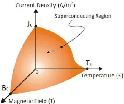
2.1 Sketch of a three dimensional critical surface of a Type I superconductor. 6 2.2 Sketch of a Type II superconductor critical magnetic fields as a function

of temperature. . . 7 2.3 Phase diagram of Helium-4 for low temperatures [6]. . . 8 2.4 a) Density of helium,ρ, as a function of temperature. b) Specific heat

of helium at constant pressure,cp, as a function of temperature. Both plots were calculated following the liquid-vapour saturation line using HEPAK® database. . . 9 2.5 a) Plot of the specific entropy of helium as a function of temperature.

b) Plot of the viscosity of helium as a function of temperature. Both plots were calculated following the liquid-vapour saturation line using HEPAK® database. . . 10 2.6 Heat transfer regimes observed at the surface of a heater placed

verti-cally in an open bath of saturated liquid helium at 4 K, for heat fluxes of 0.5 to 250 kW/m2[8]. . . 11 2.7 Plot of the steady state heat transfer regimes in He I. NC: Nucleate

Convection, NB: Nucleate Boiling, FB: Film Boiling. q_C: Critical heat flux to enter NB.q∗: Critical heat flux to enter FB.qr: Critical heat flux to recover from FB to NB [9]. . . 12 2.8 Ratio of the density of the normal and superfluid components [6]. . . . 14 2.9 Plot of the effective thermal conductivity of He II in the Landau regime,

calculated with thermal properties from Hepak®database, for a cylin-drical channel of 0.1 mm diameter. . . 17 2.10 Plot of the superfluid thermal conductivity, also known as f−1function.

LIST OFFIGURES

2.11 Sketch of the temperature discontinuity caused by Kapitza conductance at the interface solid-He II [6]. . . 19 2.12 Results compiled by V. Sciver for the Kapitza conductance [6] . . . 20 2.13 Typical steady state heat transfer curve for a metal surface in a duct

filled with He II [6].q∗: Critical heat flux to enter the film boiling regime.

q_R: Critical heat flux to recover to the Kapitza conductance regime. . . 21

3.1 Cross-section of the superconducting cable stacks used in the main dipole magnets of the LHC. . . 24 3.2 Rutherford cable structure. a) Top view. b) section. c)

Cross-section of an individual strand. d) Detailed view of the Nb-Ti filaments embedded in the copper matrix. . . 24 3.3 Sketch of the three layer polyimide insulation scheme used in LHC

dipole magnets [8]. . . 25 3.4 Sketch of the eddy currents generated in the Rutherford cable by

chang-ing magnetic field. The dots indicate the couplchang-ing resistance between adjacent strands [8]. . . 26 3.5 Schematics of the experimental setup. . . 27 3.6 Rutherford cable with half a strand removed, to accommodate a

tem-perature sensor. . . 27 3.7 Picture of the prepared Cernox®temperature sensor, electrically

insu-lated wiring using a polyimide capillary and transparent epoxy glue around the sensor itself. . . 28 3.8 a) Picture of the Rutherford cable instrumented with the Cernox®

tem-perature sensor depicted in Figure 3.7. b) Picture of the instrumented cable insulated using the three polyimide layer instulation scheme illustrated in Figure 3.3. . . 28 3.9 Picture of the cable stack sample composed of four Rutherford cables.

The second cable counting from above is instrumented using a Cernox® temperature sensor. . . 29 3.10 Picture of the sample holder made out of two half cylinders of fibreglass

epoxy. The sample is clamped using the stainless steel bolts on the side of the sample holder. . . 29 3.11 Plot of the temperature of the cable stack sample and the He II bath as

a function of time. . . 30

4.1 Plot of the effective thermal conductivity in the Gorter-Mellink regime as a function of|∇T|, calculated forT =1.8 K andγ =5×10−2K/m. 34

LIST OFFIGURES

4.2 3D plot of the effective thermal conductivity in the Gorter-Mellink regime as a function of T and|∇T|, calculated forγ=5×10−2K/m. . 35 4.3 Plot of the critical value of|∇T|as a function of temperature, calculated

ford=1×10−4m.γ(T)is used to define the value of|∇T|at which the transition between the Landau and Gorter-Mellink regime occurs. . 37 4.4 3D plot of the combined thermal conductivityKL,GM(T,|∇T|),

calcu-lated ford =1×10−4m. a) Normal scale. b) Logarithmic scale which changes the shape of the thermal conductivity for better illustration. . 38 4.5 Schematic of the experimental setup used by Van Sciver to study the

transient heat transport in He II [21]. . . 40 4.6 Experimental results from Van Sciver [21]. . . 40 4.7 One dimensional geometry used in simulation to compare with

experi-mental data from Van Sciver. . . 41 4.8 Plot of the evolution of the temperature profile of Van Sciver’s

exper-iment, calculated using the model derived in Section 4.3. The experi-mental data from Van Sciver [21] is also plotted for comparison. . . 41 4.9 Schematic of the channel geometry used in [22]. . . 42 4.10 Two dimensional geometry used in simulation to compare with

experi-mental data from [22]. . . 42 4.11 Plot of the temperature increase calculated using the model derived in

Section 4.3, for the boundary conditions indicated in Figure 4.10. The experimental data from [22] is plotted for comparison. The temperature limitT_λ is indicated by the dashed line. . . 43 4.12 Geometry and boundary conditions of a one dimensional channel

heated along its length. . . 43 4.13 Plot of the time evolution of the temperature atx =0 mm in the channel

depicted in Figure 4.12. . . 44 4.14 Plot of the time evolution of the temperature profile of the channel

depicted in Figure 4.12. . . 44 4.15 Plot of the time evolution of the temperature gradient profile of the

channel depicted in Figure 4.12. . . 45 4.16 Plot of the time evolution of the thermal conductivity profile of the

channel depicted in Figure 4.12. . . 45

LIST OFFIGURES

5.2 3D model of the spiral channels of He II, present in between the strands of the Rutherford cables. . . 48 5.3 Geometry and boundary conditions used in simulation to represent the

Rutherford cable in the dipole magnets of the LHC. . . 49 5.4 Temperature calculated as a function of time at the centre of the He II

channel and the top copper sheet. a)Normal time scale; b) Logarithmic time scale. The values of the parameters used were the same as in Table 5.1, with the exception that 85% ofqinwas used. . . 50 5.5 a) Temperature profile calculated along the centre of the He II channel

depicted in Figure 5.3. b) Temperature profile calculated along the centre of the top copper sheet depicted in Figure 5.3. . . 51 5.6 Temperature calculated as a function of time at the centre of the He II

channel depicted in Figure 5.3, for different heat inputs. . . 51 5.7 Temperature calculated as a function of time at the centre of the He II

channel depicted in Figure 5.3, for different Kapitza constants. . . 52 5.8 Temperature calculated as a function of time at the centre of the He II

channel depicted in Figure 5.3, for different percentage of He II in the polyimide insulation. . . 52 5.9 Plot of the measured and calculated temperature at the centre of the He

II channel depicted in Figure 5.3 as a funcion of time. The values of the parameters used were the same as in Table 5.1, with the exception that 85% ofq_inwas used. . . 53

A.1 Plots of the critical heat flux (a) and the superfluid critical velocity (b) as a function of temperature, calculated for different diameters. These values define the point at which the transition between the Landau and Gorter-Mellink regime occurs. . . 59 A.2 Plots of the superfluid critical velocity as a function of the diameter. The

line calculated with the developed model assumesT =1.8 K. Redrawn from [6]. . . 60

L

IST OF

T

ABLES

C

H

A

P

T

E

R

1

I

NTRODUCTION

1.1

CERN and the Large Hadron Collider

The European Organization for Nuclear Research (CERN) was founded in 1954, situated on the Franco-Swiss border close to Geneva. The acronym CERN was derived from "Conseil Européen pour la Recherche Nucléaire", the provisional council for setting up the research center, established by 12 European governments in 1952. The main purpose of CERN was and still is to provide the infrastructure needed for fundamental nuclear research, making its results generally available. Sixty years after being founded it counts with 21 member states and is the world’s largest particle physics center.

CHAPTER 1. INTRODUCTION

Figure 1.1: Layout of the CERN accelerator complex [1].

The third stage of acceleration is the PS, which increases the kinetic energy of the protons up to 28 GeV, ready for injection into the Super Proton Synchrotron (SPS). In addition the PS supplies proton beams to three different experiments, as indicated in Figure 1.1 e.g. the East Area where the beam is used in fixed-target experiments.

The fourth stage of acceleration is the SPS which increases the kinetic energy of the protons up to 450 GeV, before injection in the LHC. The SPS also provides 400 GeV proton beams to several fixed-target experiments. The last stage of ac-celeration is the LHC, which intakes two proton beams circulating in opposite directions. It increases the kinetic energy of the proton beams up to 7 TeV, to produce proton-proton collisions reaching an energy of 14 TeV. The collisions take place at four interaction points around the LHC where the ATLAS, CMS, ALICE and LHC-b detectors are installed, see Figure 1.1. The detectors measure properties such as energy, momentum, and charge of the particles created in the collisions. The data collected provides a way to better understand how matter behaves at a

1.2. DIPOLE MAGNETS IN THE LHC

fundamental level. As indicated in Figure 1.1, ions can be circulated in the LHC, namely lead nuclei are collided with an energy up to 1150 TeV. These type of collisions aim to reproduce the extreme temperature and energy density believed to have existed a fraction of a second after the Big Bang.

CERN has greatly contributed to state of the art fundamental nuclear research with the discovery of neutral currents in 1973, the discovery of W and Z bosons in 1983, the isolation of antihydrogen atoms in 2010, and the discovery of the Higgs boson in 2012 [1].

1.2

Dipole Magnets in the LHC

The LHC consists of about 9600 magnets of which 1232 are superconducting dipole magnets, used to guide the beams around the accelerator ring. The dipole magnets are a crucial part of a circular accelerator because the strength of the magnetic field they are able to generate is a limiting factor on the maximum collision energy. In the case of the LHC the magnetic field must be approximately 8.3 T to allow for 14 TeV collisions. If room temperature magnets were used instead of superconducting magnets the accelerator would have to be 120 km in circumference and would consume 40 times more energy [1].

CHAPTER 1. INTRODUCTION

The dipole magnets used in the LHC are made of niobium-titanium (NbTi) superconducting cables. To operate at the required magnetic field the magnets are cooled to a temperature of 1.9 K using superfluid helium. Each dipole magnet in the LHC weighs about 35 tonnes and is 15 m long. In total approximately 37600 tonnes of material needs to be kept at 1.9 K, requiring a very powerful cryogenic system. Figure 1.2 shows the main components of the dipole magnets used in the LHC. The superconducting coils together with the iron yoke are immersed in a superfluid helium bath kept at 1.9 K and 0.13 MPa. A heat exchanger pipe with superfluid helium at 1.86 K and 1.6 kPa runs along the iron yoke to extract the heat generated during operation.

1.3

Scope of the Thesis

The thermal stability of superconducting magnets is a crucial part of the operation of the LHC. The dipole magnets in the LHC need to operate below certain critical temperature, magnetic field, and current density values in order to remain in the superconducting state. This is explained in more detail in Section 2.1. It is very important to understand how heat is extracted from the magnets in order to estimate stability margins for its operation. The phenomena responsible for the heat deposition on the magnets can be categorized into steady state and tran-sient. The stability margins are closely related to the character of the phenomena responsible for the heat deposition in the coils. Up to now the experimental work reported helps understand how heat is transported in steady state conditions [2]. The study of heat transport in He II in transient conditions relies heavily on simulation. In this thesis it is investigated how heat is transported in transient con-ditions from inside the magnet coils towards the heat sink of a liquid helium bath. Both measurements and numerical simulations have been performed to study the phenomena governing the heat extraction process. A new numerical model was developed describing the heat transport in He II in the Landau and Gorter-Mellink regimes. At the end a comparison is made between the measurements and the numerical results obtained with the developed model. The comparison of the obtained measurements with the numerical results demonstrates the validity of the developed numerical model.

C

H

A

P

T

E

R

2

T

HEORY

This Chapter focuses on the thermal properties of helium. It describes the heat transfer mechanisms present in helium I and helium II often referred to as the normal phase and the superfluid phase, respectively. Special attention is given to the superfluid phase due to its relevance in both the experimental and simulation work presented in this thesis. A short introduction on superconductivity is pro-vided to help understand how a material enters the superconductive state and what is required for it to remain in that state.

2.1

Superconductivity

CHAPTER 2. THEORY

Figure 2.1: Sketch of a three dimensional critical surface of a Type I superconductor.

current density the material transitions into the normal conducting state.

In 1957 John Bardeen, Leon Cooper, and John Robert Schrieffer published a microscopic theory [3] explaining superconductivity, often referred to as the "BCS theory" after the names of the authors. The core of this theory is the assumption that, at very low temperatures, the electrons in a superconductor can be attracted to each other. This arises from the fact that an electron travelling through the material will attract nearby positive charges in the lattice. This region of higher density of positive charge attracts a nearby electron with opposite spin and momentum. Thus the two electrons form what is called a Cooper pair, which has spin zero. The Cooper pairs strongly overlap and form a highly collective condensate state. When this state is reached the energy required to break a Cooper pair is related to the energy necessary to break all the pairs. This means that possible collisions with the lattice due to thermal motion are not enough to disturb the condensate. Thus the electrons can travel through the material without experiencing any resistance. Allowing the formation of screening currents that never dissipate and expel the magnetic field from the interior of the superconductor. These currents are referred to as supercurrents. It is easy to understand from this picture that there must be a critical point at which the thermal motion of the lattice no longer allows the existence of the condensate state. At that point the material is no longer in the superconducting state.

Besides the superconductors described by BCS theory commonly called Type-I,

2.2. LIQUID HELIUM

there is a different kind of superconductors called Type-II. These behave as Type-I superconductors until the critical surface of the Meissner phase is reached. Instead of transitioning directly to the normal conducting state, Type-II superconductors enter an intermediate state. This behaviour was described by Ginzburg and Lan-dau in 1950 in a phenomenological theory [4]. In 1957 Abrikosov introduced the idea that in the intermediate state, the superconductor has the ability of letting some magnetic flux penetrate its interior without loosing superconductivity [5]. In this state it is energetically more favourable to form supercurrent vortices which let some magnetic flux pass through the superconductor, instead of expelling it completely.

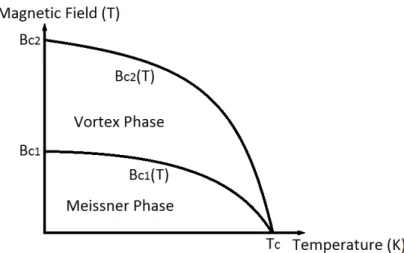
The intermediate state is often referred to as the vortex state. Figure 2.2 shows a sketch of the critical magnetic field as a function of temperature for a certain current density. If the current density dependency is taken into account the two critical lines in Figure 2.2 become two critical surfaces similar to Figure 2.1.Above the second critical surface superconductivity breaks down as in Type-I supercon-ductors. Type-II superconductors can withstand considerably higher temperature, magnetic field, and current density when compared with Type-I superconductors. For this reason Type-II superconductors are suitable for large scale projects such as superconducting dipole magnets.

Figure 2.2: Sketch of a Type II superconductor critical magnetic fields as a function of temperature.

2.2

Liquid Helium

CHAPTER 2. THEORY

between helium I (He I) and helium II (He II). Throughout this thesis the word helium is used to refer to its most common isotope,4He.

2.2.1

Helium as a Cooling Fluid

Liquid helium is the cryogenic liquid that most closely represents an ideal fluid. This near perfect behaviour is due to the fact that helium exhibits a very weak intermolecular potential. As a result of this both gaseous and liquid helium can be described in classical terms until the superfluid transition. In contrast to this classical behaviour, below the superfluid transition liquid helium can only be described using quantum mechanics. The same is valid for the solid phase of helium. In this Section a summary of the helium phase diagram is provided, focussing on the characteristics that are different from regular fluids. Figure 2.3 shows the phase diagram of helium.

Like most materials it has two phase-coexistence lines, namely: solid-liquid, liquid-vapour, and a critical point. In addition to the conventional characteristics, several unique features can be observed in the helium phase diagram. Liquid helium can exist in two completely different liquid phases, He I and He II. He I is a normal liquid and its characteristics can be described using classical fluid mechanics. He II, also called the superfluid phase, has remarkable properties such

Figure 2.3: Phase diagram of Helium-4 for low temperatures [6].

2.2. LIQUID HELIUM

as a very low viscosity and a very high thermal conductivity, even when compared with a high-conductivity solid such as copper [6]. The transition between these two phases is a second order phase transition, meaning that there is no latent heat associated with it. As a consequence it is not possible for He I and He II to coexist in equilibrium.

Helium does not have a triple point where solid liquid and vapour phases can coexist. This feature is related to the fact that the solid phase of helium only exists if external pressure is applied. For a more detailed description of the helium phase diagram, see [6].

2.2.2

Thermal Properties of Liquid Helium

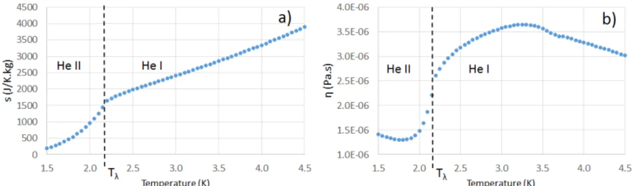
The most relevant thermal properties of liquid helium are plotted in Figures 2.4 and 2.5 using a helium data base called HEPAK®. As highlighted in these figures a change in all the thermal properties is clearly visible at 2.17 K. The changes in the thermal properties are related to the phase transition from He I to He II. It is called the lambda transition due to the distinct shape of the specific heat depicted in Figure 2.4 b), resembling the Greek letterλ(lambda).

As shown in Figure 2.4 a) in He II the density increases with temperature until reaching a maximum value after Tλ. In He I the density decreases with increasing

temperature as expected for a classical fluid. Above Tλ the specific heat shown

in Figure 2.4 b) has a value close to what would be expected for an ideal gas. The specific heat reaches a maximum value at Tλ which is five to six orders of

magnitude higher than that of copper in the same temperature range. Below T_λ the specific entropy shown in Figure 2.5 a) is proportional to the third power of the temperature whereas above T_λit is linear with temperature. This change in

CHAPTER 2. THEORY

Figure 2.5: a) Plot of the specific entropy of helium as a function of temperature. b) Plot of the viscosity of helium as a function of temperature. Both plots were calculated following the liquid-vapour saturation line using HEPAK®database.

slope is characteristic of a second-order phase transition. As stated in Section 2.2.1 this means that there is no latent heat associated with the conversion of He I into He II, and the two phases cannot coexist in equilibrium.

Figure 2.5 b) shows the dynamic viscosity, which in the case of He I has values similar to those of the vapour phase of a classical fluid. In the case of He II two methods can be used to measure the dynamic viscosity. The first method consists of using a viscosimeter to measure the pressure drop in the laminar regime through a micro-tube [6]. The second method measures the drag exerted on a disk in rotation [6]. For a classical fluid these two methods of measurement give the same result. In the case of He II they give very different results. The first method measures zero viscosity whereas the second method measures the values depicted in Figure 2.5 b). The lack of agreement between the two methods was one of the facts that inspired the creation of a new model consisting of two fluids to explain the extraordinary behaviour of He II. The main feature of this model is the assumption that He II is composed of two fluid components, the normal component and the superfluid component [7]. The first component has the viscosity measured using the rotating disk and the later has zero viscosity. A more detailed description of the two-fluid model is given is Section 2.2.4.

2.2.3

Heat Transport Mechanisms in Helium I

As mentioned in Section 2.2.1, He I can be treated as a classical fluid. This Section provides a brief description of the heat transfer mechanisms present in He I. The lower limit in terms of temperature of these mechanisms is T_λ, below which He I becomes He II. The upper limit is the critical point, depicted in Figure 2.3. The heat transfer in He I can be described using three different regimes.

2.2. LIQUID HELIUM

Figure 2.6: Heat transfer regimes observed at the surface of a heater placed vertically in an open bath of saturated liquid helium at 4 K, for heat fluxes of 0.5 to 250 kW/m2[8].

As depicted in Figure 2.6 there is a transient regime present at the very begin-ning of the heating process, i.e. for short times. As time elapses new heat transfer regimes can establish depending on the heat flux being applied. For low enough heat fluxes a steady state nucleate boiling (NB) takes place after the transient regime. For higher heat fluxes a metastable nucleation regime takes place after the transient regime, eventually reaching a steady state heat transfer regime called film boiling (FB).

CHAPTER 2. THEORY

takes place until a certain critical heat flux,q∗, at which a vapour film forms and blankets the heater. Since the thermal conductivity of the vapour layer is very small compared to the thermal conductivity of the liquid, the surface is thermally insulated from the liquid. Consequently the temperature of the heated surface suddenly jumps. In the film boiling regime the heat transfer to the liquid is much less efficient than in any of the other regimes.

Figure 2.7 summarizes the steady-state behaviour of the heat transfer regimes mentioned before by plotting the temperature increase at the heated surface as a function of the heat flux. It is clearly visible in Figure 2.7 that the slope of the plot changes each time a critical heat flux is reached, meaning a new regime is entered. The hysteresis shown in Figure 2.7 is due to the activation of nucleation sites where bubbles form. This means that the heat flux required to recover from film boiling,qr is lower than the critical value needed to enter it in the first placeq∗. As is visible in Figure 2.7, it is not possible to recover from nucleate boiling back to natural convection once the nucleation sites are activated.

Figure 2.7: Plot of the steady state heat transfer regimes in He I. NC: Nucleate Convection, NB: Nucleate Boiling, FB: Film Boiling.q_C: Critical heat flux to enter NB.q∗: Critical heat flux to enter FB.qr: Critical heat flux to recover from FB to NB [9].

2.2. LIQUID HELIUM

2.2.4

Heat Transport Mechanisms in Helium II

In this Section the heat transport mechanisms present in He II are derived starting from the two-fluid model. The laminar and the turbulent heat transfer regimes are usually referred to as the Landau and the Gorter-Mellink regimes, respectively. Besides these two regimes the phenomenon of Kapitza conductance and the film boiling regime play an important role in the heat transfer in He II. Up to now both phenomena are treated from a practical point of view and a satisfactory theoretical description is still missing [6].

2.2.4.1 The Two-Fluid Model

The two-fluid model is a description of the fluid mechanics of He II, namely the heat and mass transport. Originally proposed by Tisza [7] and later refined by Landau [10], it describes He II as a mixture of two interpenetrating fluid components. The normal fluid component, containing all the entropy and viscosity in the liquid, and the superfluid component with zero viscosity and zero entropy.

It is important to mention that He II is often called a superfluid because the word was used to describe its extraordinary behaviour before the two-fluid model was formulated. After the introduction of the two-fluid model, it is more correct to say that liquid helium can be found in two distinct liquid phases: He I, and He II. Furthermore, He II has two components: normal fluid, and superfluid.

The properties of the fluid as a whole are a combination of the properties of the two components. Thus the density of He II is the sum of the densities of the two components,

ρ =ρs+ρn . (2.1)

The density of He II is temperature dependent, as well as the normal and superfluid densities. Figure 2.8 shows the ratio of normal and superfluid densities as a function of temperature.

As mentioned before in this Section the the two-fluid model assumes that the normal fluid component carries all the entropy, so the entropy of He II is written as:

ρs=ρnsn , (2.2)

CHAPTER 2. THEORY

Figure 2.8: Ratio of the density of the normal and superfluid components [6].

velocity of the normal componentvn, as:

S=ρsvn . (2.3)

From equation (2.3) the heat fluxqcarried by the normal component can be expressed as:

q=ρsTvn . (2.4)

Equation (2.4) is central to the heat transfer in He II, and will be used in the subsequent Sections to help understand the different heat transfer regimes. The total momentum equation for He II can be written using two velocity fields, one for each component [6],

ρv =ρnvn+ρsvs . (2.5)

Equation (2.5) describes the connection between the two fluid components. In a closed system of He II, without any forced convection by means of a pressure difference, it can be assumed a zero net mass flow, which simplifies equation (2.5) to:

ρnvn+ρsvs =0. (2.6) As equation (2.4) shows a heat flux causes the normal component of the fluid to flow. This in turn causes the superfluid component to flow in the opposite direction, as expressed by equation (2.6). This counter-flow is often called internal

2.2. LIQUID HELIUM

convection and is the origin of the remarkable heat transport ability of He II. The dynamics of He II changes depending on the relative velocity of the two components. This leads to the existence of two different heat transfer regimes, one for low and one for high relative velocities [6].

2.2.4.2 The Laminar Regime: Landau Regime

In this derivation of the laminar regime, only the first order effects are taken into account due to the weak contribution of second order effects to the heat transport [11]. A description of interesting second order phenomena, like second sound, can be found in [11]. In the laminar regime the two fluid components are connected by the continuity equation [6]:

∂ρ

∂t +∇ ·(ρv) = 0 . (2.7)

The total momentum equation of He II is similar to the case of a classical incompressible fluid, with the exception that the viscosity is only associated with the normal fluid component,

∂ρv

∂t =−∇p+η∇

2_v

n , (2.8)

where p stands for pressure and η is the viscosity of the normal fluid com-ponent. For low relative velocities it is assumed that the superfluid velocity is consequence of a potential and it is possible to prove that it is a chemical potential [2]. Under this assumption Landau defined the following relation between the superfluid velocity and the temperature and pressure gradients:

∂vs

∂t =s∇T−

1

ρ∇p. (2.9)

In the case of a one dimensional channel, under steady-state conditions equa-tion (2.9) becomes the well known London equaequa-tion, commonly used to describe the fountain effect [6]:

dp dx =ρs

dT

dx . (2.10)

From the momentum equation (2.8) together with equations (2.5) and (2.9) it is possible to describe the time evolution of the two velocity fieldsvn andvs, as:

ρn

∂vn

∂t =−ρss∇T−

ρn

ρ ∇p+η∇

2_v

CHAPTER 2. THEORY

and

ρs∂vs

∂t =ρss∇T−

ρs

ρ ∇p. (2.12)

The total momentum equation (2.8) under steady state conditions leads to the Poiseuille equation:

∇p=η∇2vn . (2.13)

For a channel with constant cross-section, taking the London equation (2.10) into account, equation (2.13) can be solved. Giving rise to a relation between the temperature gradient and the velocity of the normal component:

dp dx =ρs

dT dx =−

β

d2ηvn , (2.14) wheredrepresents the diameter of the channel andβis a constant that depends on the geometry. It is equal to 32 for a pipe with circular cross-section and equal to 12 for two parallel plates. Using the heat flux equation (2.4) and the relation found in equation (2.14) it is possible to relate the heat flux with the temperature gradient, as:

q =−d2

β ρ2s2T

η

dT

dx . (2.15)

This equation resembles a Fourier type law, with a temperature dependent effective thermal conductivity of:

KL(T) = d 2

β ρ2s2T

η , (2.16)

where the L subscript stands for Landau. Figure 2.9 shows the temperature dependency of effective thermal conductivity in the Landau Regime for a 0.1 mm diameter channel. The effective thermal conductivity is a combination of various thermal properties and varies approximately asT12d2.

Figure 2.9 shows a thermal conductivity 100 times higher than pure copper, for the same temperatures [12]. From equation (2.16) it may seem that increasing the diameter would allow a higher heat flux for the same temperature gradient. In fact there is a limit to this, which defines a critical velocity. Above this velocity turbulence starts to develop in the superfluid component and the effective thermal conductivity has lower values.

2.2. LIQUID HELIUM

Figure 2.9: Plot of the effective thermal conductivity of He II in the Landau regime, calculated with thermal properties from Hepak®database, for a cylindrical channel of 0.1 mm diameter.

2.2.4.3 The Turbulent Regime: Gorter-Mellink Regime

When the relative velocity of the two fluid components reaches a certain critical value turbulence starts to develop in the superfluid component. This behaviour is described by Gorter and Mellink [13] and gives rise to a dissipative interaction between the two fluid components. To account for this dissipation mechanism, an extra term called mutual friction is defined as:

Fns = Aρnρs|vn−vs|3, (2.17)

where A is the temperature dependent Gorter-Mellink coefficient. The mu-tual friction term is introduced in equations (2.11) and (2.12), resulting in two momentum equations for the turbulent regime:

ρn∂vn

∂t =−ρss∇T−

ρn

ρ ∇p+η∇

2_v

n−Fns . (2.18)

and

ρs∂vs

∂t =ρss∇T−

ρs

ρ∇p+Fns . (2.19)

From equations (2.18) and (2.19), following the same approach as in the last Section, it is possible to show that the temperature gradient expression has an extra term related to the mutual friction:

dT dx =−

β

d2ηvn−

Aρn

s |vn−vs|

CHAPTER 2. THEORY

Assuming a zero net mass flow and using equation (2.4) the relation between temperature gradient and heat flux for a one dimensional channel can be written as:

dT dx =−

βη

d2_ρ2_s2_Tq−

Aρn

ρ3 ss4T3

q3. (2.21)

The first term on the right hand side of the equation is the same as found in the Landau regime. The second term is a consequence of the mutual friction between the two fluid components, and varies with the third power of the heat flux. Thus for high heat fluxes the first term is negligible, and equation (2.21) can be simplified to:

q3 =−f−1(T)dT

dx , (2.22)

with

f−1(T) = ρ 3 ss4T3

Aρn

, (2.23)

where f−1(T)is the so called superfluid thermal conductivity function. Fig-ure 2.10 shows f−1 as a function of temperature with a distinct maximum at around 1.9 K.

It is important to note that even though f−1is referred to as superfluid thermal conductivity, it does not have units of thermal conductivity. Nonetheless it trans-lates how efficiently heat can be transported in He II. The understanding of this function can be useful for example when deciding the operation temperature of a superconducting magnet coil in He II. A wise choice would be to operate slightly

Figure 2.10: Plot of the superfluid thermal conductivity, also known as f−1function. Calculated for saturation conditions using the Hepak® database.

2.2. LIQUID HELIUM

below the maximum of the f−1function. In case of a local hot spot, the increase in temperature would improve the heat transfer and help to recover to nominal operation conditions.

2.2.4.4 Kapitza Conductance

When heat is transferred from a solid material to He II the first thermal barrier is the solid-liquid interface. This phenomenon is often referred to as Kapitza conduc-tance, from the name of the physicist who first identified it in 1941 when studying the heat transfer from a copper block to He II [14]. This conductance causes a temperature discontinuity at the solid-He II interface, depicted in Figure 2.11, which arises from the different acoustic properties of the two materials.

Figure 2.11: Sketch of the temperature discontinuity caused by Kapitza conduc-tance at the interface solid-He II [6].

The Kapitza conductance is defined empirically as the ratio between the heat flux and the temperature difference at the interface, as:

h_K0 = lim ∆_T→0

q

∆_T , (2.24)

where q is the heat flux and ∆_{T is the temperature difference between the}

surface and the He II. The subscript 0 refers to the limit case where ∆_{T → 0.}

Experimentally this conductance is treated as the relation between the finite values ofqand∆_{T, as:}

hK = _∆q

T . (2.25)

CHAPTER 2. THEORY

Figure 2.12: Results compiled by V. Sciver for the Kapitza conductance [6]

authors report results that lay between the two theoretical limits, as Figure 2.12 shows.

The Kapitza conductivity depends on parameters such as surface roughness and shape. Due to the lack of agreement between theoretical predictions and measurements, usually the Kapitza conductance is determined experimentally. Van Sciver [6] compiled existing experimental results for copper between 1.8 K and 2.0 K, and identified the Kapitza conductance,h_K (W/K.m2), to be within the range:

400T_b3≤hK ≤1100T_b3, (2.26)

where the subscriptbindicates the bath temperature. It is important to consider the effect of Kapitza conductance when doing experimental or simulation work, due to the limit it constitutes to the amount of heat transferred from a solid material to He II. It can help distinguish between a temperature measurement of

2.2. LIQUID HELIUM

the solid material or the He II. The Kapitza conductance is taken into account in the simulation work presented in Chapter 5.

2.2.4.5 Film Boiling Regime

Above a certain critical heat flux,q∗, a film of helium vapour forms at the heated surface. As in the classical film boiling regime there is a recovery heat flux q_R

smaller thanq∗, which allows the Kapitza conductance regime to be re-established. This causes hysteresis in the heat transfer curve, as shown in Figure 2.13. Contrary to what happens in He I this hysteresis is not observed in all the He II heat transport experiments [6].

In the film boiling regime the heat transfer is very ineffective due to the low thermal conductivity of the vapour film that insulates the heated surface from the He II bath. The heat transfer coefficient associated with film boilinghf bdepends on several physical parameters including heater geometry, orientation, bath tem-perature, and pressure [6]. Typicallyh_{f b}is 10 to 100 times smaller than the Kapitza conductance coefficienth_K which can be problematic in cryogenic applications. For this reason film boiling is the most limiting heat transfer regime in He II, unfortunately it is one of the least understood due to its complexity. The region close to the heated surface can contain up to three helium phases: He II, He I, and vapour. This makes the physical interpretation of the heat transfer much more

CHAPTER 2. THEORY

difficult than the case of single phase He II. Furthermore, there is no theory capable of describing the multiphase boiling processes [6]. For engineering applications this heat transfer regime can be expressed using the linear relation:

q=h_{f b}(Ts−Tb) , (2.27)

where the subscriptssandbstand for surface and bath, respectively. The film

boiling heat transfer coefficienth_{f b}has a typical value in the order of 250 to 1000W/m2K[9].

C

H

A

P

T

E

R

3

E

XPERIMENT

In the experimental work presented in this Chapter, a stack of NbTi Rutherford cables was placed in a bath of He II representing the operating conditions of a dipole magnet in the LHC. With the goal of investigating the transient heat transfer in He II, the cable stack is heated and the time evolution of its temperature is recorded. It is explained how heat has been generated in the cable stack and how its temperature is measured. As an introduction to the investigated heat transfer problem the experimentally used structure of the Rutherford cables is described in detail.

3.1

Superconducting Rutherford Cables

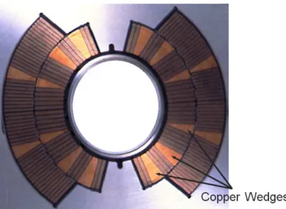
The coils placed around the beam pipe, indicated in Figure 1.2, are made up of superconducting Rutherford cable stacks. The cable stacks are spaced using copper wedges, as shown in Figure 3.1, to assure the homogeneity of the magnetic field generated [2].

CHAPTER 3. EXPERIMENT

Figure 3.1: Cross-section of the superconducting cable stacks used in the main dipole magnets of the LHC.

As stated in Section 2.1, during operation the values of temperature, magnetic field, and current density need to be kept below certain critical values for the magnets to remain in the superconducting state. If in a particular region of the cable any of these critical values is exceeded, that region becomes normal conducting. With a very high current still going through the cable the temperature in that region will escalate due to joule heating. This normal conductive region can rapidly grow and potentially lead to the meltdown of a dipole magnet. This cascade process is called quench. The copper matrix in which the NbTi filaments are embedded plays an important role in case of a quench, serving as a temporary bypass for the high current.

Figure 3.2: Rutherford cable structure. a) Top view. b) section. c) Cross-section of an individual strand. d) Detailed view of the Nb-Ti filaments embedded in the copper matrix.

3.2. AC-LOSSES IN RUTHERFORD CABLES

The Rutherford cables in the magnets are electrically insulated from each other using three polyimide layers, as depicted in Figure 3.3. The insulation scheme itself is a topic of ongoing research with the goal of combining good electrical insulation with good cooling performance. It is possible to recover from a quench without damaging the magnets if enough cooling power is provided. For this reason a better understanding of how heat can be extracted from the magnets is crucial for the operation of the LHC.

Figure 3.3: Sketch of the three layer polyimide insulation scheme used in LHC dipole magnets [8].

3.2

AC-losses in Rutherford Cables

CHAPTER 3. EXPERIMENT

Figure 3.4 shows a sketch of how an eddy current can circulate in the Rutherford cable strands.

The Rutherford cable design is optimised to reduce the amount of heat losses generated by the mechanisms mentioned above. A detailed explanation of the techniques used to reduce these losses can be found in [19]. Nonetheless heat can be generated in the cables using an alternating magnetic field. In the experimental work presented in this Chapter AC-losses were used to generate heat in the NbTi Rutherford cables.

Figure 3.4: Sketch of the eddy currents generated in the Rutherford cable by chang-ing magnetic field. The dots indicate the couplchang-ing resistance between adjacent strands [8].

3.3

Experimental Setup

A pressure regulated cryostat was used to keep a He II bath at constant temperature ranging from 1.8 K to T_λ at saturation conditions. The main component of the setup in Figure 3.5 is the superconducting coil, used to generate an alternating magnetic field. The superconducting coil was connected to the power grid and operated at 230 VRMS @ 50 Hz. This connection was controlled using a trigger system.

During the experiment a stack of Rutherford cables was placed at the center of the superconducting coil. The temperature of the cable stack and the temperature of the helium bath were monitored using two temperature sensors connected to a Keithley 3706Amicrovoltmeter. A level gauge was used to monitor the height of the helium bath. During the experiment a column of about 300 to 1000 mm of helium was present above the cable stack sample.

3.4. SAMPLE PREPARATION

Figure 3.5: Schematics of the experimental setup.

3.4

Sample Preparation

The cable stack sample placed at the center of the superconducting coil, depicted in Figure 3.5, is composed of four 20 cm long NbTi Rutherford cables. One of the cables in the stack was machined as illustrated in Figure 3.6 to accommodate a temperature sensor. A bare chip Cernox® sensor was used to measure the tem-perature of the cable. The sensor consists of a resistive element whose resistance varies with temperature.In situcalibration of the sensor allows the translation of a measurement of resistance into temperature. The well known four-wire technique was used to measure the resistance, with a constant current of 10µA. The voltage drop was measured using a Keithley 3706Amicrovoltmeter.

CHAPTER 3. EXPERIMENT

Figure 3.7: Picture of the prepared Cernox® temperature sensor, electrically insu-lated wiring using a polyimide capillary and transparent epoxy glue around the sensor itself.

During the experiment heat is generated by means of currents induced in the Rutherford cable, therefore it is crucial to electrically insulate the temperature sensor from the cable to guarantee that the voltage drop measured on the sensor is only caused by temperature.

The sensor was insulated using epoxy glue and a thin polyimide capillary, see Figure 3.7. Due to its small dimensions the sensor was prepared under an optical microscope. Two wires were soldered to each leg of the sensor and the soldering points were insulated with epoxy glue. The thin polyimide capillary was placed over the cables, leaving only the sensor exposed. The head of the sensor was insulated using epoxy glue. The sensor is housed in a glue drop of approximately 1 mm in diameter at the end of the polyimide capillary. The sensor was inserted in place of one of the strands in the cable, as Figure 3.8 a) illustrates.

Each of the four cables was hand-wrapped using three layers of polyimide tape, following the insulation scheme of Figure 3.3 used in the LHC dipole magnets.

Figure 3.8: a) Picture of the Rutherford cable instrumented with the Cernox® temperature sensor depicted in Figure 3.7. b) Picture of the instrumented cable insulated using the three polyimide layer instulation scheme illustrated in Fig-ure 3.3.

3.5. EXPERIMENTAL RESULTS

Figure 3.9: Picture of the cable stack sample composed of four Rutherford ca-bles. The second cable counting from above is instrumented using a Cernox® temperature sensor.

Figure 3.8 b) shows the instrumented cable insulated with polyimide tape. The first two layers have a thickness of 50µm and the third layer is 69µm thick. Figure 3.9 shows the cable stack sample with the instrumented cable.

The cables in the stack were clamped together using a sample holder made out of fibreglass epoxy, depicted in Figure 3.10. The sample holder needs to be made out of non-electrically-conducting material to avoid shielding the sample from the magnetic field, and to prevent additional heat from being generated close to the sample.

Figure 3.10: Picture of the sample holder made out of two half cylinders of fibre-glass epoxy. The sample is clamped using the stainless steel bolts on the side of the sample holder.

3.5

Experimental Results

CHAPTER 3. EXPERIMENT

a period of typically 10 to 300 seconds. During the experiment the temperature of the bath and the temperature of the sample are recorded each 60 ms using the Keithley 3706Amicrovoltmeter. The Cernox®sensor placed inside the sample was calibratedin situusing the pressure reading of the control unit that regulates the pressure of the cryostat. The pressure was converted into temperature based on the fact that the bath was in saturation conditions. This leads to an accuracy in the temperature measurements of 2 mK using the Cernox®sensor. The experimental results shown in Figure 3.11 were obtained with a bath temperature of 2.164± 0.002 K in saturation conditions. When the coil is turned on the temperature of the sample increases approximately 8±2 mK above the temperature of the bath.

Steady state conditions are reached very quickly when heating the sample, due to the high thermal conductivity of He II. To study the thermal response of the sample it is important to have a large amount of measurements while its temperature rises. In order to obtain a temperature increase which takes a few seconds, the bath was kept at temperatures very close toT_λ. At such temperatures the specific heat of He II increases considerably as Figure 2.4 b) shows, which extends the time it takes to reach steady state conditions. Figure 3.11 shows how the temperature of the sample increases as a function of time, the trigger signal, as well as the bath temperature of 2.164±0.002 K. After 10 seconds the sample reaches a constant temperature of 2.173±0.002 K. The coil is turned off after 300 seconds and the temperature of the sample drops quickly back to the bath temperature.

Figure 3.11: Plot of the temperature of the cable stack sample and the He II bath as a function of time.

C

H

A

P

T

E

R

4

N

UMERICAL

M

ODEL

This Chapter describes the numerical model developed in this thesis. First it is shown how the governing equations can be derived from the equations presented in Chapter 2. It is explained how the thermal conductivities of the Landau and Gorter-Mellink regimes are crucial in understanding the heat transport in He II. The model developed is validated by comparison with existing experimental data from different authors. Finally the model is used to obtain simulation results on how the heat is transported from the Rutherford cable strands, through the He II channels, into the He II bath.

4.1

Governing Equations

The energy equation used in this numerical model can be deduced starting from the energy equation for incompressible fluids:

ρcp

∂T

∂t +v· ∇T

=−∇ ·q, (4.1)

where ρ is the density of He II, cp is the specific heat of He II at constant pressure, andqis the heat flux. As stated in Section 2.2.4.1 a zero net mass flow can be assumed in the heat transport process and expressed as:

CHAPTER 4. NUMERICAL MODEL

This means that He II as a whole is stationary and the two fluid components move internally, thus equation (4.1) can be simplified, as:

ρcp∂T

∂t =−∇ ·q. (4.3)

Equation (4.3) is used to study the heat transport in solids. In this numerical model He II is treated as a solid material with a special thermal conductivity, which is derived in the next Section. As described in Sections 2.2.4.2 and 2.2.4.3 there are heat equations for the Landau and Gorter-Mellink regimes that relate the heat flux with the temperature gradient:

• Equation (2.15), the Landau regime:

q =−d 2

β ρ2s2T

η

dT dx .

• Equation (2.22), the Gorter-Mellink regime:

q3 =−f−1(T)dT

dx .

The substitution of the heat fluxes from equations (2.15) and (2.22) in equa-tion (4.3) provides a way of studying the heat transport in both the Landau and Gorter-Mellink regimes. In Section 4.2 it is shown how these equations were used to develop a new numerical model which covers the two regimes and describes the heat transfer in He II in transient conditions.

4.2

Effective Thermal Conductivities

In general the heat transport in solids is studied using a thermal conductivity to expresses the relation between the heat flux and the temperature gradient. Typically, this thermal conductivity is temperature dependent. Since this model considers He II to be equivalent to a solid, it is relevant to explore how its thermal conductivity looks like. First this Section focuses on how equations (2.15) and (2.22) can be rearranged in order to obtain effective thermal conductivities that represent either the Landau or the Gorter-Mellink regime. Secondly it is shown how both effective thermal conductivities can be combined into a single thermal conductivity which covers the two regimes.

4.2. EFFECTIVE THERMAL CONDUCTIVITIES

4.2.1

The Landau Regime

The effective thermal conductivity of the Landau regime for a cylindrical channel, derived in Section 2.2.4.2, depends on both the temperature and the channel diameter, as stated in equation (2.16):

K_L(T) = d 2

32

ρ2s2T

η .

As shown in Figure 2.9 the effective thermal conductivity increases with tem-perature and is proportional toT12.

4.2.2

The Gorter-Mellink Regime

Originally, equation (2.22) was defined by Gorter and Mellink [13] for a one dimensional channel. It has been shown that equation (4.4) with m = 3.4 fits experimental data better than equation (4.4) wherem=3 [6].

qm =−f−1(T) dT

dx . (4.4)

In this Section, for simplicity the equations are derived assumingm =3, at the end it is shown how the equations look like withm =3.4. Equation (2.22) can be generalized into the two or three dimensional case using the temperature gradient instead of the temperature derivative, leading to:

q≡ −f−1/3₍

T)∇T1/3

. (4.5)

It is very important to understand the meaning of the power1_{/3of the} tem-perature gradient present in equation (4.5) to study the heat transfer in the Gorter-Mellink regime. In this work it is interpreted as being a vector with magni-tude|∇T|1_/3_{and with the direction of the temperature gradient, as:}

∇T1/3 _{≡ |∇}

T|1/3_∇d

T , (4.6)

where ∇dT is the unit vector with the direction of the temperature gradient. Furthermore, equation (4.6) can be rearranged to relate directly to the temperature gradient, as:

∇T1/3_=|∇

T|1/3 ∇T

|∇T| =|∇T|

−2_/3_∇

T . (4.7)

Thus the heat equation (2.22) can be rewritten as:

q≡ −f−1/3_(T)∇T1_/3 ₌₋f

−1_/3

(T)

CHAPTER 4. NUMERICAL MODEL

where it is easy to recognize the effective thermal conductivity as being:

K_GM(T,|∇T|) = f

−1_/3_(T)

|∇T|2_/3 . (4.9)

The Gorter-Mellink effective thermal conductivity depends on temperature through the f−1(T)function, and also depends on the magnitude of the tempera-ture gradient|∇T|. Ifm =3.4 in equation (4.4), the effective thermal conductivity of the Gorter-Mellink regime becomes:

K_GM(T,|∇T|) = f

−1_/3.4_(T)

|∇T|3.43.4−1

. (4.10)

Equation (4.9) may suggest that the effective thermal conductivity increases indefinitely as the magnitude of the temperature gradient decreases. In fact for small enough temperature gradients the heat flux is proportional to the temper-ature gradient, meaning that equation (4.9) is no longer suitable to describe the heat transfer.

Up to now equation (4.5) is used to study the heat transfer in the Gorter-Mellink regime assuming a|∇T|always larger than a constant residual value,γ[20]. It is a sensible solution to guarantee numerical stability of the calculations when a high heat flux is applied. In the first steps of calculation, when |∇T|is very small, it is replaced by the residual valueγ. When |∇T|is larger thanγnumerical stability is no longer an issue. This approach requires the value ofγto be set and optimised depending on the heat flux and geometry being investigated. Figure 4.1 shows the effective thermal conductivity of the Gorter-Mellink regime as a function of|∇T|.

Figure 4.1: Plot of the effective thermal conductivity in the Gorter-Mellink regime as a function of|∇T|, calculated forT =1.8 K andγ=5×10−2K/m.

4.2. EFFECTIVE THERMAL CONDUCTIVITIES

In this example the temperature is chosen to beT =1.8 K and the residual gradient is set toγ=5×10−2K/m.

For values of|∇T|smaller thanγas indicated in Figure 4.1 the thermal con-ductivity is constant. A bad estimation of the value ofγcan lead to results discon-nected to what is observed experimentally. Underestimating the value ofγcould lead to an extremely high thermal conductivity. In contrast, overestimating the value ofγcould result in a thermal conductivity independent of the temperature gradient. As stated before in this SectionKGM depends on temperature through the f−1(T)function. Figure 4.2 shows how KGM depends both on temperature and on the magnitude of the temperature gradient, for γ = 5×10−2 K/m as Figure 4.1.

In Figure 4.2 it is possible to recognize the distinct shape of the f−1(T)function, compare Figure 2.10, with a maximum close to 1.9 K and vanishing to zero as T approachesTλ. The step in Figure 4.1 for|∇T|smaller thanγbecomes a plateau

in Figure 4.2.

CHAPTER 4. NUMERICAL MODEL

4.2.3

Combined Thermal Conductivity

As explained in Sections 2.2.4.1 and 2.2.4.2, heat is carried by the normal fluid component, which is set in motion by a temperature gradient. There is a critical velocity at which a transition from the Landau to the Gorter-Mellink regime occurs. This means that the critical velocity can be interpreted as being equivalent to a critical temperature gradient.

In Section 4.2.2 the introduction of a constant residual gradientγaccounts for the fact that, as|∇T| → 0, the thermal conductivity should no longer depend on |∇T|. This gives rise to a thermal conductivity that is only temperature dependent, for|∇T|smaller thanγ, that can be written as:

K_GM(T,γ) = f

−1_/3.4_(T)

γ3.43.4−1

. (4.11)

If the magnitude of the temperature gradient|∇T| is smaller than a certain critical value the heat transfer is described by the Landau regime. This means that whenγis equal to a critical|∇T| the thermal conductivities of the Landau and Gorter-Mellink regimes take the same value. It is possible to derive howγlooks like by first setting the thermal conductivities of the two regimes equal:

K_GM(T,γ) = KL(T) . (4.12)

More explicitly:

f−1_/3.4_(T)

γ3.43.4−1

=K_L(T) . (4.13)

Equation (4.13) can be rearranged to show a parameterγwhich is temperature dependent:

γ(T) = f

− 1

3.4−1 (T)

K

3.4 3.4−1 L (T)

= f−3.41−1 (_T)

d2

β ρ2s2T

η

−_3.43.4₋₁

. (4.14)

This leads to a parameterγ(T)which is the critical|∇T|. The critical gradient

γ(T)is translated into a critical heat flux and a critical velocity in appendix A. Figure 4.3 shows how the parameter γvaries with temperature. The value ofγ

decreases as the temperature increases, which means that it is easier to enter the turbulent regime as T approachesT_λ.

4.2. EFFECTIVE THERMAL CONDUCTIVITIES

Figure 4.3: Plot of the critical value of|∇T|as a function of temperature, calculated ford =1×10−4m.γ(T)is used to define the value of|∇T|at which the transition between the Landau and Gorter-Mellink regime occurs.

With a temperature dependent critical gradientγ(T), it is possible to write a combined thermal conductivity that covers both the Landau and Gorter-Mellink regimes, as:

K_L,GM(T,|∇T|) =

  

KL(T) |∇T| <γ(T)

K_GM(T,|∇T|) |∇T| ≥ γ(T) . (4.15) Based on the value of|∇T|the thermal conductivity is either described by the Landau regime or by the Gorter-Mellink regime. This combined thermal conduc-tivity is presented in a 3D plot in Figure 4.4, which shows how it depends onT

and|∇T|. Both a normal and a logarithmic scale are used to facilitate the identifi-cation of the functions that compose the combined thermal conductivity,K_L,GM.

In Figure 4.4 a) the maximum value of thermal conductivity is the same as in the Landau regime. Thus its profile resembles the shape ofKL shown in Figure 2.9. As indicated in Figure 4.4 b) the edge from which the value of thermal conductivity abruptly decreases has the shape of γ(T) that connects the two regimes, see Figure 4.3. For|∇T| beyond this edge the thermal conductivity is the same as in the Gorter-Mellink regime. It decreases as |∇T| increases, and has a shape resembling the f−1(T)function depicted in Figure 2.10.

CHAPTER 4. NUMERICAL MODEL

Figure 4.4: 3D plot of the combined thermal conductivityK_L,GM(T,|∇T|), calcu-lated ford=1×10−4m. a) Normal scale. b) Logarithmic scale which changes the shape of the thermal conductivity for better illustration.

4.3

Model Implementation in COMSOL

COMSOL Multiphysics®is a software developed to perform numerical calculation on heat transfer, structural mechanics, fluid mechanics, among other branches of physics. COMSOL®lets the user add a geometry, choose the physics involved in the simulation, and select the type of numerical solver to be used, e.g.: steady state or transient. This Section shows how the model developed in Sections 4.1 and 4.2 is implemented in COMSOL®to study transient heat transfer in He II. In this model He II is treated as a solid material, therefore COMSOL® uses equation 4.3 to compute the time evolution of the temperature. To calculate using this equation the geometry introduced in COMSOL®needs to be discretized in nodes. This is done using a mesh which has a size either automatically generated depending on the physics or defined by the user. Ideally the size of the mesh should be the largest possible without affecting the numerical results, in order to use efficiently the computing power available. In the simulations presented in this work the size of the mesh was defined manually, due to its influence in the stability of the calculations.