Individual tree growth models for eucalyptus in northern Brazil

ABSTRACT: The diameter and height growth model is one of three submodels used for simulating individual tree growth. In Brazil, there are few studies on the dimensional growth of individual trees be they native or exotic species, despite their potential. This study aimed to evaluate diameter and height growth models for individual trees for eucalyptus stands and to validate the best fitting model. Tree diameter and height data were obtained from 48 permanent plots of unthinned stands of Eucalyptus grandis × Eucalyptus urophylla hybrid located in northern Brazil. The evaluation of the diameter and height growth models was based on adjusted coefficient of determination, standard error of estimate as a percentage, trend, root mean square error and Akaike Information Criterion. Analysis also included distribution of residual percentage, statistical significance and signs of the coefficients. The Lundqvist–Korf model provided the most accurate estimates for diameter and height growth, in comparison with the other models, providing better statistical values, greater proximity to observed values and better distribution of residual percentages. The use of this type of model is feasible and can result in significant improvements in the accuracy of yield estimates. Keywords: growth and yield models, forest growth prediction, tree-level models

Received April 25, 2013

Accepted January 21, 2014 1

Federal University of Itajubá – Natural Resources Institute, C.P. 50 – 37500-903 – Itajubá, MG – Brazil.

2_{Federal University of Viçosa – Dept. of Forest Engineering –} 36570-000 – Viçosa, MG – Brazil.

3_{Federal University of Espírito Santo – Dept. of Forest} Engineering – 29550-000 – Alegre, ES – Brazil. *Corresponding author <fabrina@unifei.edu.br> Edited by: Paulo Cesar Sentelhas

Individual tree growth models for eucalyptus in northern Brazil

Fabrina Bolzan Martins1_{*, Carlos Pedro Boechat Soares}2_{, Gilson Fernandes da Silva}3

Introduction

Dimensional growth in terms of diameter and height is one of the three constituents of an individual tree model and is subject to complex interactions (Andreassen and Tomter, 2003; Soares and Tomé, 2002). It is influenced by growth vigor, past growth conditions, microenvironment, genetic traits and competitive status (Tomé and Burkhart, 1989).

In models at the level of the individual tree, growth is often estimated via the potential growth function or growth equations (Davis et al., 2005). In the potential growth function, growth is obtained by multiplying potential growth (Pg) by a modifier function (fm) (Biging and Dobbertin, 1992; Soares and Tomé, 1997). Pg describes the maximum possible growth that a tree can attain, whereas fm describes the decrease in growth potential due to competition (Kiernan et al., 2008). In contrast, growth equations (or functions) use tree attributes (tree size, competition indices, crown ratio, vigor), stand attributes (age, site index, stand basal area) and site characteristics as predictor variables, all combined in a single equation (Uzoh and Oliver, 2006).

Several equations are used to estimate growth, including linear or polynomial equations (Kiernan et al., 2008), the Bertalanffy equation (Vanclay, 1994), the Richards equation (Amaro et al., 1998), the Gompertz equation, the logistic equation and the exponential equation (Zeide, 1993) in addition to nonlinear functions (Zhang et al., 2004). However, the superiority of modifier functions over growth equations (or functions) has not been demonstrated.

Many studies have been conducted on model growth in diameter and height at the individual tree level in forests in the USA and Europe (Biging and Dobbertin, 1992; Lynch and Murphy, 1995; Tomé and Burkhart,

1989; Vospernik et al., 2010). In Brazil, there have been few studies estimating forest growth at this level. Existing studies refer to native species such as Cabralea canjerana (Durlo, 2001), araucaria (Araucaria angustifolia) (Chassot et al., 2011), cedar (Cedrela fissilis) (Durlo et al., 2004)and certain species from the Amazon region (Silva et al., 2002). On the other hand, there are no models that estimate growth at the individual tree level for planted commercial species. Because of the importance of the genus Eucalyptus in Brazil, with more than four million hectares planted (ABRAF, 2011) and the gap in growth modeling at individual tree level, the aim of this study was to evaluate and compare various diameter and height models for individual Eucalyptus grandis × Eucalyptus urophylla trees.

Materials and Methods

The study was conducted in Monte Dourado, in the state of Pará, Brazil (0º53’22” S, 52º36’6” W, 65 m a.s.l.). The region has a tropical monsoon climate (Am), with an average annual precipitation of 2.115 mm and a short dry season between Sept and Nov, according to the Köppen classification. The average annual temperature is 26.4 ºC, and average relative humidity ranges between 80 % and 85 % (Martins et al., 2011).

To estimate Ht for the remaining trees, a hypsometric equation was used, which was fitted to the site (Martins et al., 2011) (eq. 1):

Ht = 36.9876 – 30.4340

.

.

.

ln(t))1.388275 ₍₁₎

( 2

R =83.7%; S_y.x%= R211.79%).

where dbh = diameter outside bark as measured 1.30 m above ground level (cm); Hd = average height of dominant trees (m); t = age (months); 2

R % = adjusted coefficient of determination (percentage); and S_y.x% = standard error of estimate (percentage), both computed in the original units of the dependent variable (m). The heights of dominant trees (Hd) were also used to classify the productive capacity by means of site indices (SI) (eq. 2) via the guide curve method (Campos and Leite, 2009), which correlates the height of dominant trees with the stand age at an index age.

ln SI = ln(Hd) + 14.8802

.

where t_i = index age (60 months); t = age (months). The thresholds used for plot classifying into productivity classes were: i) low productivity class (SI = 20, which represents the center value of the class): plots with Hd ≤ 23 m with index age of 60 months; ii) average productivity class (SI = 26): plots with Hd

between 23 and 29 m; and iii) high productivity class (SI = 32): plots with Hd _{> 29 m.}

Seven models for estimating the diameter and height growth of an individual tree were evaluated (Table 2). As the growth models used in this study have a projection structure (t → t₊₁), the Durbin-Watson test (dw) was applied to verify autocorrelation in these models, which all have a similar autoregressive structure (Gujarati, 2004). This analysis evaluated linear and nonlinear relationships. Models were fitted independently to each productivity class (Martins et al., 2011) (SI = 32, SI = 26 and SI = 20).

Two model fitting tools were used in this study: the SAS software MODEL procedure (Statistical Analysis System, version 8.0, 2001), with maximum likelihood fitting for nonlinear estimation, and the nonlinear estimation procedure from Statistica software (Statsoft, version 7.0, 2008), which uses a variant of the Gauss-Newton method to estimate the parameters of nonlinear regression by the least squares method.

The fit of the equations of the seven models was verified with the following statistics: the adjusted coefficient of determination ( 2

R ), trend (BIAS), standard error of estimate in percent (S_y.x%), root mean square error (RMSE) and Akaike Information Criterion (AIC) (Gujarati, 2004):

( )

2 _{1 a1 R}

R = − −

(

)

(

)

i i i

y y y y R 1 2 1 2 2 ˆ

1

1 1 − − − = p n n a (5)

(

)

n

y

y

BIAS

i i i

∑

−

=

ˆ

(

)

i i i

x y (7) 1 ) ˆ ( 2 1 − ∑ − = = n y y RMSE i n i i

2 _{( ˆ )}

exp ∑ − + =  =     ⋅ (9)

where y_i = i-th observed value for the dependent variable; y_i = i-th estimated value for the dependent variable; y_i = mean observed value for the dependent variable; n-1 = degrees of freedom of the total in the analysis of variance; n-p-1 = degrees of freedom of the residual from the analysis of variance of the regression, p = number of coefficients and n = number of observations.

The model resulting in the greatest 2

R , least BIAS, S_y.x%, RMSE and AIC was selected as the best model. In addition to the above statistics, graphs were developed to compare observed diameters and heights with those estimated by models, as well as graphs of the distribution of residual percentages (res%) relating to estimated diameters and heights (Vanclay, 1994). Table 1 – Characteristics of Eucalyptus grandis × Eucalyptus

urophylla located in Monte Dourado, in the state of Pará, Brazil.

Age (months) 24 - 72

Diameter at breast height: dbhat 1.30 m (cm) 4.0 - 29.4 Average diameter: q (cm) 7.3 - 18.4 Total height: (Ht) (m) 8.5 - 34.1 Dominant height: (Hd) (m) 13.1 - 34.8 Basal area (m² ha–1_{) 4.7 - 27.2}

Volume (m³ ha–1_{) 23.8 - 353.9}

Density (trees ha–1_{) 760 - 1180} ∑

= / n

i=1 dbh n dbh ; ∑ 2 = / =1 n q dbh n

i

Table 2 – Models used for estimating diameter and height growth for individual eucalyptus trees.

Number Model Author

1

(

)

= ⋅ 0 21 11

2 1 exp t t

Y Y Pienaar and Schiver (1981)

2 1 2 2 1 2 t t Y Y A A b e           = ⋅  +

 

.

.

3 ₍1 2 2_{) (}1 2 1₎

0 0

2 1

1 exp t 1 exp t

Y =Y+_ b_{b b− ⋅} − b_{b b− ⋅} _+e

+ +

  Logistic / Amaro et al. (1998)

4 _{( )}1 _{( )}1

3 3

1 2 2 1 2 1

0 0

2 1

1 exp t 1 exp t

Y Y

b b

b b b b

b b e − ⋅ − ⋅     = + − +  _{+ +} 

  Richards / Zeide (1993)

5 (0 1 2) (0 1 1)

2 1 exp exp

t t

Y =Y+ b b+ ⋅ − b b+ ⋅ +e Schumacher / Campos and Leite (2009)

6 2 1 1 2

2 1

1 1

LnY LnY BAI

t t

b   b e

= + ⋅ − + ⋅ +

 

Adapted Schumacher equation Campos and Leite (2009)

7 2 1 0 1 2 3

2 1

1 1

Y Y BAI SI

t t

b b b b e

   

= +_ + ⋅ − + ⋅ + ⋅ _+

 

 

Linear / adapted from Bella (1971) and Campos and Leite (2009)

Y₂ = diameter (cm) or height (m) in future age; Y₁ = diameter (cm) or height (m) in current age; t₂= future age (months); t₁= current age (months); BAI = basal area index = 2 2 i d BAI =

q ; di = dbh subject-tree (cm) and q = quadratic mean diameter (cm); b0. b1. b2. b3 = coefficients to be estimated; and e = random error.

The best-fitting model to represent diameter and height growth was also tested with independent data. Simulation was performed on 18 permanent plots whose evaluation was based on the RMSE. The homogeneity of variance was tested between the observed values of diameter and height and the values estimated by the best model in each productive capacity class using a Bartlett’s test (H₀ = homogeneous variances versus H₁ = heterogeneous variances). This same Bartlett’s test can be used to test the absence of normality, and this test was used in this study. The observed mean values of diameter and height were compared, using a t-test, with the mean values estimated by the best model in each productive capacity class.

Results

In this study, all equations referring to the models assessed for the variables diameter and height in all three productivity classes provided values that were very close to each other according to the relevant statistics ( 2

R , BIAS, S_y.x%, RMSE and AIC) (Table 3). The models with the best fit were those for SI = 32, followed by SI = 26 and finally SI = 20. Individual tree diameter and height growth models are among the basic and essential components of forest growth models (Sánchez-González et al., 2006).

The best estimates of diameter were obtained using models 1, 2 and 6. Only a few equations showed significant autocorrelation according to a dw test (Table 3). In these cases, it is incorrect to compare the 2

R

values for the estimators with those reported by other studies because the ordinary least squares estimators are biased (Gujarati, 2004).

Generally, lower estimates of 2

R (0.28 to 0.83) were found by Sterba and Monserud (1997) and by

Andreassen and Tomter (2003) for the basal area increment of Pinus sylvestris, Picea abies and Betula sp. Tomé and Burkhart (1989) and Adame et al. (2008) also found lower estimates (0.51 to 0.54) for the diameter increment of Eucalyptus globulus and Quercus pyrenaica (0.44). Lower estimates were also obtained by Soares and Tomé (1997) (0.99) using the Lundqvist-Korf (L-K) model for the quadratic dbh mean of Eucalyptus globulus. In analyzing BIAS, models 1 and 7 (SI = 32, 26 and 20), 2 (SI = 32 and 20) and 6 (SI = 32) overestimated diameter in a small range of values, whereas models 3, 4, and 5 (SI = 32, 26 and 20), 2 (SI = 26) and 6 (SI = 26 and 20) underestimated diameter. Soares and Tomé (1997) obtained similar negative estimates of BIAS (-0.038 to -0.016 cm) for the quadratic dbh mean of Eucalyptus globulus, the same as had been observed by Sánchez-González et al. (2006) for the diameter increment of Quercus suber. Härkönen et al. (2010) found values higher than those found in this study; these authors used other models to estimate the diameter growth of Betula pendula (-0.70 cm) and Betula pubescens (-0.80 cm).

The highest estimates found for S_y.x% and RMSE were ±5.98 (S = 20) and 0.699 cm (S = 26), respectively, both for model 5, whereas the lowest were ±3.03 in SI = 32 and 0.46 cm in SI = 20, respectively, both for model 2. Sánchez-González et al. (2006) and Härkönen et al. (2010) found higher values of S_y.x% and RMSE for the growth of Quercus suber (±40.82), Picea abies (±14.4 and 2.8 cm) and Pinus sylvestris (±17.0 and 3.4 cm) and similar values for Betula pendula (± 3.8 and 6.3 cm) and Betula pubescens (±5.8 and 3.5 cm).

All equations based on the models provided very similar values for height for all the statistics assessed. The best equations involving height were those based on models 2 and 6, as they provided higher 2

lower BIAS, S_y.x%, RMSE and AIC values in comparison with the other models. As in the case of diameter, several equations showed autocorrelation (Table 3).

The statistic R2 was higher in model 2 in all productivity classes, with estimates between 0.97 and 0.99 with values referring to S = 20 and 32, respectively. Lynch and Murphy (1995) and Mabvurira and Miina (2002) found similar estimates of 2

R for the height

growth of Pinus echinata (0.96 to 0.98) and Eucalyptus grandis (0.94) with different models. Filipescu and Comeau (2007) and Mette et al. (2009) obtained lower estimates for Picea glauca (0.47 to 0.86), Abies alba (0.18 to 0.89) and Picea abies (0.39 to 0.82), using different height increment equations.

The lowest estimates of BIAS were found for models 2, 3 and 4. As in the case of diameter, the Table 3 – Statistics used for evaluating the seven diameter and height growth models.

Model Author/Type Site índex _R2 _{BIAS S}

y.x% RMSE AIC dw

diameter 1 Pienaar and Schiver

SI = 32 0.9836 0.00328 ± 3.31 0.5308 1.2839 1.9609

SI = 26 0.9818 0.00330 ± 3.69 0.5330 1.2857 1.7849

SI = 20 0.9752 0.00331 ± 4.70 0.5283 1.2809 1.7208

2 Lundqvist-Korf

SI = 32 0.9875 4.26x10–6 _{± 3.03 0.4737 1.2276 1.7603} SI = 26 0.9825 -5.28x10–5 _{± 3.48 0.4802 1.2338 1.7470} SI = 20 0.9724 6.24x10–6 _{± 4.39 0.4615 1.2158 1.7379} 3 Logistic

SI = 32 0.9721 -0.00028 ± 4.33 0.6942 1.4150 2.0661

SI = 26 0.9724 -0.00024 ± 4.82 0.6968 1.4881 1.8687

SI = 20 0.9696 -0.00003 ± 5.12 0.5777 1.3366 1.8339

4 Richards

SI = 32 0.9720 -0.00035 ± 4.34 0.6944 1.4863 2.0648

SI = 26 0.9723 -0.00026 ± 4.83 0.6970 1.4894 1.8675

SI = 20 0.9706 -0.00002 ± 5.13 0.5778 1.3375 1.8334

5 Schumacher

SI = 32 0.9697 -0.00209 ± 4.80 0.6948 1.4842 2.0646

SI = 26 0.9612 -0.00411 ± 5.65 0.6990 1.4903 1.8562

SI = 20 0.9586 -0.00486 ± 5.98 0.5775 1.3354 1.8346

6 adapted Schumacher

SI = 32 0.9871 0.00052 ± 3.85 0.6081 1.2109 1.6942

SI = 26 0.9801 -0.00012 ± 3.59 0.6290 1.2277 1.4255ns SI= 20 0.9702 -0.00063 ± 4.53 0.5498 1.2192 1.4256ns 7 Linear

SI = 32 0.9860 0.00035 ± 3.92 0.4921 1.3718 1.6957ns SI = 26 0.9800 0.00013 ± 3.71 0.5249 1.3973 1.6682ns SI = 20 0.9700 0.00069 ± 4.74 0.4882 1.3041 1.6803ns

Height 1 Pienaar and Schiver

SI = 32 0.9865 0.00145 ± 2.34 0.4733 1.2270 1.8099

SI = 26 0.9791 0.00166 ± 3.16 0.5526 1.3071 1.7583

SI = 20 0.9732 0.00199 ± 3.63 0.6940 1.4833 1.7438

2 Lundqvist-Korf

SI = 32 0.9886 0.00070 ± 2.00 0.4682 1.2224 1.7945

SI = 26 0.9869 0.00084 ± 2.53 0.5622 1.2988 1.7688

SI = 20 0.9706 0.00018 ± 3.25 0.5324 1.2862 1.7639

3 Logistic

SI = 32 0.9750 -0.00017 ± 2.96 0.7038 1.4984 2.0172

SI = 26 0.9750 -0.00019 ± 3.49 0.7634 1.5854 1.7491

SI = 20 0.9667 -0.00005 ± 4.10 0.7224 1.5245 1.7209

4 Richards

SI = 32 0.9749 -0.00025 ± 2.97 0.7048 1.5009 2.0115

SI = 26 0.9751 -0.00014 ± 3.47 0.7635 1.5865 1.7486

SI = 20 0.9667 -0.00004 ± 4.09 0.7224 1.5248 1.7209

5 Schumacher

SI = 32 0.9480 -0.00210 ± 4.60 0.7011 1.4935 2.0320

SI = 26 0.9429 0.00398 ± 5.21 0.7628 1.5836 1.7516

SI = 20 0.9480 -0.00311 ± 5.04 0.7204 1.5206 1.7300

6 adapted Schumacher

SI = 32 0.9878 -0.00122 ± 2.07 0.4947 1.2446 1.8439

SI = 26 0.9847 -0.00179 ± 2.71 0.5927 1.3530 1.8029

SI= 20 0.9700 -0.00228 ± 3.43 0.6043 1.3670 1.4017ns 7 Linear

SI = 32 0.9750 0.00393 ± 2.30 0.6065 1.3729 1.8410

SI = 26 0.9636 0.00159 ± 2.83 0.6543 1.4272 1.7804

equations based on models 1, 2 and 7 (SI = 32, 26 and 20) had positive BIAS values, demonstrating that these models tended to overestimate height growth in all three productivity classes despite the limited range. Models 3, 4 and 6 (SI = 32, 26 and 20), as well as 5 (SI = 32 and 20), produced negative estimates, underestimating height growth. Lynch and Murphy (1995) found higher BIAS values for Pinus echinata (0.13 to 0.25 m), the same trend observed by Mabvurira and Miina (2002), who found a BIAS of 0.19 m for Eucalyptus grandis. Härkönen et al. (2010) found negative estimates of BIAS for the height growth of Pinus sylvestris (-0.2 m) and Betula pendula (-0.1 m) but positive estimates for Betula pubescens (0.5 m) and Picea abies (1.1 m).

The lowest S_y.x% and RMSE values were found for the equations based on model 2 and model 6, both for S = 20 and S = 32 (Table 3). By comparison, Härkönen et al. (2010) found higher values of height growth for Picea abies (±18.5 %), Pinus sylvestris (±20.7 %), Betula pendula (±34.5 %) and Betula pubescens (±26.7 %).

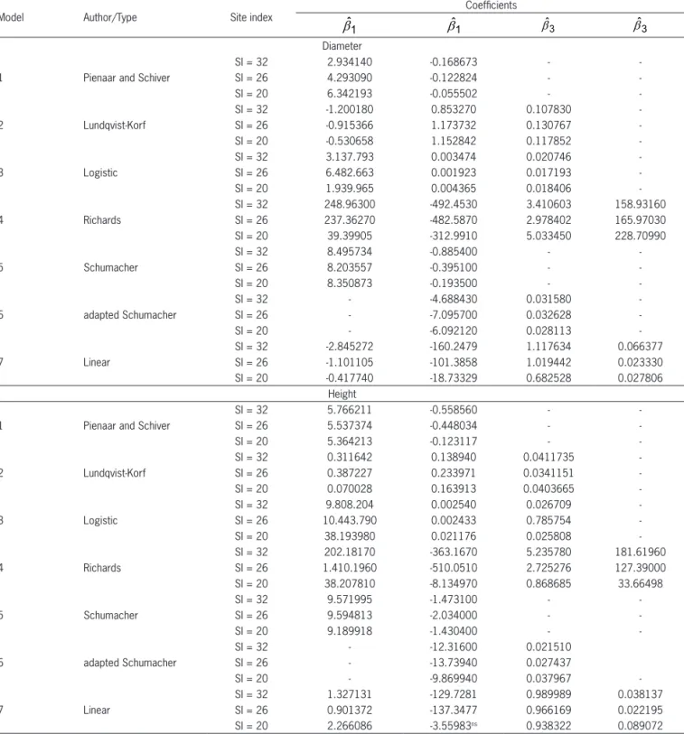
Virtually, all coefficients of the equations were significant (p ≤ 0.05) (Table 4). The sign of the coefficient of age was negative (models 1, 5, 6 and 7), indicating that growth increases with increasing age until a certain point is reached (the index age), whereas other variables remain constant. These findings are biologically consistent and similar to results found in other growth studies at the individual tree level (Lee et al., 2004; Subedi and Sharma, 2011). Additionally, the signs of the site index and competition index were positive for diameter and height growth in all productivity classes. These results show that trees will reach greater diameters and greater heights in better sites (Adame et al., 2008) where there is a greater opportunity to compete. Thus, these results are consistent with the literature (Mabvurira and Miina, 2002; Lee et al., 2004; Sánchez-González et al., 2006) and are biologically realistic, reflecting good estimates for all diameter and height growth models evaluated in this study.

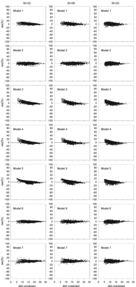
The values estimated by the equations based on the seven diameter growth models were concentrated near the 1:1 line (Figure 1), indicating a good estimation capability for all three productivity classes. Models 3, 4 and 5 had a slight tendency to overestimate smaller diameters and underestimate larger diameters. This trend was also observed by Sterba and Monserud (1997), Mabvurira and Miina (2002), Mette et al. (2009) and Vospernik et al. (2010). These trends are common and difficult to explain, with overestimation occurring more often in low-density stands and underestimation more often in high-density stands (Vospernik et al., 2010).

Models 1, 2 and 6 performed well in terms of the assessed statistics (Table 3) and managed to accurately estimate tree diameter in all three productivity classes. Nevertheless, model 1 underestimated the diameters of the larger trees, those in SI = 32. model 6 overestimated the diameters of the larger trees in a narrow range in SI = 20. This result is similar to that reported by Filipescu and Comeau (2007) for Picea glauca.

The residual percentages for diameter growth (Figure 2) were well distributed for models 2, 6 and 7 in all three productivity classes. Despite its good statistical performance, model 1 showed a slight deficiency in its residual distribution, underestimating trees of larger diameter in all three productivity classes. Models 3, 4 and 5 had a marked deficiency in their residual distributions and failed to capture the growth trends for trees of smaller and larger diameters (S = 32, 26 and 20). These three models overestimated the small-diameter region and underestimated the large-diameter region. This trend was similar to that reported by Härkönen et al. (2010). For diameter growth, the equations based on models 2, 6 and 7 succeeded in accurately estimating diameter variation in all three productivity classes and did not exceed a residual percentage of ± 20 %. Nevertheless, model 2 showed better estimates in terms of the assessed statistics and had well distributed residuals.

Wykoff (1990), Kiernan et al. (2008) and Monty et al. (2008) obtained similar results, for the basal area increment, diameter growth and circumference, respectively, for different species. Andreassen and Tomter (2003) found variations of more than 20 % for the basal area increment in Picea abies, Pinus sylvestris and Betula sp and Härkönen et al. (2010) reported a ± 17% for Pinus sylvestris, ± 26 % for Betula pubescens and ± 35 % for Betula pendula.

For height growth (Figure 3), the points were close to the 1:1 line in all models. As in the case of diameter growth, a tendency of the models to produce incorrect estimates was noted in height growth for trees of smaller and larger sizes. Model 1 overestimated smaller and larger trees in all three productivity classes. Model 2 slightly overestimated larger trees, with a wider range in SI = 32. Models 3, 4 and 5 showed a pattern similar to each other, with little variation among the three productivity classes. SI = 32 and 26 showed overestimates for trees of smaller height, whereas SI = 20 showed overestimates for trees of smaller height and underestimates for taller trees. Models 6 and 7 showed a slight tendency to overestimate smaller trees in all productivity classes and a strong tendency to overestimate larger trees.

Results from Soares and Tomé (2002) corroborated those obtained from most of the models evaluated in this study. Soares and Tomé (2002) state that this response is due to data quality and to equation fitting, with equation accuracy decreasing as the productivity class gradually decreases. Additionally, height is a difficult variable to measure and must be obtained indirectly via hypsometric equations that, in turn, contain intrinsic inaccuracies.

Models 6 and 7 failed to estimate the endmost values of the variable height, particularly initial values smaller than 18 m.

Mette et al. (2009) and Härkönen et al. (2010) also found it difficult to estimate height growth, particularly for trees of smaller (10 m) and larger sizes (25 m). It is important to note that trees in all height classes directly influence the overall volume attained (Mette et al., 2009). Therefore, models that are incapable of capturing

Table 4 – Estimates of coefficients of equations based on the seven models assessed for diameter and height growth in each productivity class.

Model Author/Type Site index

Coefficients

1 ˆ

b bˆ1 bˆ3 bˆ3

Diameter 1 Pienaar and Schiver

SI = 32 2.934140 -0.168673 -

-SI = 26 4.293090 -0.122824 -

-SI = 20 6.342193 -0.055502 -

-2 Lundqvist-Korf

SI = 32 -1.200180 0.853270 0.107830

-SI = 26 -0.915366 1.173732 0.130767

-SI = 20 -0.530658 1.152842 0.117852

-3 Logistic

SI = 32 3.137.793 0.003474 0.020746

-SI = 26 6.482.663 0.001923 0.017193

-SI = 20 1.939.965 0.004365 0.018406

-4 Richards

SI = 32 248.96300 -492.4530 3.410603 158.93160 SI = 26 237.36270 -482.5870 2.978402 165.97030

SI = 20 39.39905 -312.9910 5.033450 228.70990

5 Schumacher

SI = 32 8.495734 -0.885400 -

-SI = 26 8.203557 -0.395100 -

-SI = 20 8.350873 -0.193500 -

-6 adapted Schumacher

SI = 32 - -4.688430 0.031580

-SI = 26 - -7.095700 0.032628

-SI = 20 - -6.092120 0.028113

-7 Linear

SI = 32 -2.845272 -160.2479 1.117634 0.066377

SI = 26 -1.101105 -101.3858 1.019442 0.023330

SI = 20 -0.417740 -18.73329 0.682528 0.027806

Height 1 Pienaar and Schiver

SI = 32 5.766211 -0.558560 -

-SI = 26 5.537374 -0.448034 -

-SI = 20 5.364213 -0.123117 -

-2 Lundqvist-Korf

SI = 32 0.311642 0.138940 0.0411735

-SI = 26 0.387227 0.233971 0.0341151

-SI = 20 0.070028 0.163913 0.0403665

-3 Logistic

SI = 32 9.808.204 0.002540 0.026709

-SI = 26 10.443.790 0.002433 0.785754

-SI = 20 38.193980 0.021176 0.025808

-4 Richards

SI = 32 202.18170 -363.1670 5.235780 181.61960 SI = 26 1.410.1960 -510.0510 2.725276 127.39000

SI = 20 38.207810 -8.134970 0.868685 33.66498

5 Schumacher

SI = 32 9.571995 -1.473100 -

-SI = 26 9.594813 -2.034000 -

-SI = 20 9.189918 -1.430400 -

-6 adapted Schumacher

SI = 32 - -12.31600 0.021510

SI = 26 - -13.73940 0.027437

SI = 20 - -9.869940 0.037967

-7 Linear

SI = 32 1.327131 -129.7281 0.989989 0.038137

SI = 26 0.901372 -137.3477 0.966169 0.022195

SI = 20 2.266086 -3.55983ns _{0.938322 0.089072}

variation in a given height range should be avoided even if they provide good estimates for the remaining height classes. Only model 2 was capable of estimating height growth for the three productivity classes with a residual percentage not exceeding ±20 %.

functional relationship and flexibility of the equation, whose coefficients have biological significance (Amaro et al., 1998).Thus this model is among the functions most commonly used to estimate growth phenomena (Burkhart and Tomé, 2012).

Crescente-Campo et al. (2010) reported serious heteroscedasticity problems in equations for the basal area increment, as well as non-normality of errorsin equations for the diameter and height increment, in contrast to the results of this study (Table 5). A Bartlett’s test indicated that the assumptions of normality were met for the observed and estimated diameters by the L-K model in all three productivity classes (p > 0.05). The same was true for height except where SI = 26. Additionally, this test confirmed homogeneity of variance for the observed and estimated diameters in all three productivity classes and for the observed and estimated heights in classes SI = 32 and SI = 20, a desirable result.

No difference (p > 0.05) was found between the observed mean values and the values estimated by the L-K model for diameter and height (S = 32 and 20). For diameter, the RMSE was less than 1 cm in all three productivity classes, a result similar to those reported

Figure 5 – Diameter and height simulated by the Lundqvist-Korf model in all three productivity classes.

Table 5 – Mean and variance related to diameters and heights observed and simulated by the Lundqvist-Korf model in all three productivity classes.

Site index Mean Variance

Obs Sim Obs Sim

Diameter

SI = 32 14.42 14.15ns _{12.42 13.12}ns SI = 26 13.18 13.06ns _{12.62 12.94}ns SI=20 10.69 10.67 ns _{9.23 9.39} ns Height

SI = 32 20.81 20.25ns _{20.06 18.41}ns SI = 26 19.10 18.23* _{20.07 17.67}* SI = 20 16.13 15.66 ns _{13.60 12.76} ns Obs = observed values; Sim = simulated values; ns= not significant; *significant at 5 % by the t-test (compares the observed mean with each estimated mean) and by the Bartlett’s test (compares the observed variance with each estimated variance) in all three productivity classes.

an underestimation of height in trees taller than 30 m (SI = 32) and in trees taller than 22 m (SI = 26). However, RMSE was 0.59 m for SI = 32 and 0.91 m for SI = 26. An error in the range of 0.50 m can be considered low and totally acceptable from the standpoint of height modeling because the top portion of the tree is typically ignored for commercial purposes. However, an error greater than 0.50 m can be harmful, as it could affect the estimation of volume. One approach to the problem of estimating height is to use hypsometric equations with simulated data with regard to diameter, as the simulation of diameter was excellent. The L-K model showed greater consistency between the statistics and biological reality and thus provided the most accurate and best fitting model for diameter and height growth.

Discussion

Although the models in this study include diameter and height explicitly as dependent variables, many studies use alternative forms of diameter and height growth as dependent variables (e.g., diameter and height increment, diameter and height growth rate, square increment and natural logarithm of each), as well as growth modifier functions (Adame et al., 2008). However, modeling the diameter and height increment is not the only alternative for predicting tree growth, and other variables have been modeled, including future diameter and height (Bueno and Bevilacqua, 2010). All are alternative approaches to estimating the increase in stem and height size. They are mathematically related, and few differences in the outcome of the modeling process are expected (Vanclay, 1994) if the assumptions regarding the error term are met (Bueno and Bevilacqua, 2010; Zhang et al., 2004).

In Brazil, the use of diameter and height as dependent variables in models to assess growth at the individual tree level is common (Chassot et al., 2011) and conceivable (Campos and Leite, 2009). Bueno and Bevilacqua (2010) compared the two approaches in modeling the diameter growth ofPinus occidentalis and

found that the estimates of future diameters (as used in this study) showed lower errors if directly projected by the model than those resulting from estimates using the increment in diameter. A possible justification is that the periodic increment varies significantly as a function of the environmental conditions of the study site (Garcia, 1988), which are extremely variable in northern Brazil. Additionally, this problem is exacerbated in rapidly growing species such as eucalyptus, as they show large increments in comparison with slowly growing species.

Growth equations can be derived directly from functions correlating diameter and height as a function of independent variables such as competition index, site, stand height and stand density (Davis et al., 2005; Lynch and Murphy, 1995). However, there has been no confirmation of the universal superiority of one dependent/independent variable over another or of

the performance of modifier functions relative to that of growth equations. The choice of one function in preference to another and the functional relationship chosen between variables (Sánchez-González et al., 2006; Soares and Tomé, 1997) will depend on the interests and convenience of the researcher (Vanclay, 1994).

A large number of growth models with numerous combinations of variables are continually evaluated and tested for a wide variety of species (Uzoh and Oliver, 2006). It becomes more difficult, however, to select the best model to estimate growth if the modeling unit is an individual tree (Davis et al., 2005) because the high resolution of this type of modeling entails problems caused by cumulative errors (Cao, 2006). Even with such difficulties, it was nevertheless possible to obtain a good estimate of diameter and height growth using model 2.

The reasons for prefering model 2 (L-K) is that this model provided better statistical estimates, as the values estimated by model 2 were close to the observed values in terms of accuracy for diameter and height growth (Figures 1 and 3). This model also showed a good distribution of residual percentages (Figures 2 and 4), and accurate estimating of diameter and height growth in all size classes (smaller, intermediate and larger trees) in all three productivity classes. Model 2 was also found to be accurate in simulating diameter and height growth in individual eucalyptus trees (Figure 5), revealing greater consistency between the statistics and biological reality and thus providing the most accurate and best fitting model for diameter and height growth.

In Brazil, individual tree growth models are still rarely used to model growth and yield. Most applications use whole-stand and size-class models. A major reason for this practice is that models on an individual tree level are considered more complex; because of this belief, users in Brazil have little experience with this type of model. However, the results presented in this study show that the use of this level of modeling is feasible and can offer significant improvements for estimating growth and yield more accurately. Moreover, it is a flexible type of model because it provides detailed information about dynamics and stand structure, including the distribution of volume by size class. From this detailed information, it is possible to correct projections for different uses of timber, sawmill, lumber, paper, plywood, charcoal, pulp and biomass and to understand how competition and the site index impact growth.

Acknowledgments

References

Adame, P.; Hynynen, J.; Cañellas, I.; Río, M. 2008. Individual-tree diameter growth model for rebollo oak (Quercus pyrenaica Willd.) coppices. Forest Ecology and Management 255: 1011-1022.

Amaro, A.; Reed, D.; Tomé, M.; Themido, I. 1998. Modeling dominant height growth eucalyptus plantations in Portugal. Forest Science 44: 37-46.

Andreassen, K.; Tomter, S.M. 2003. Basal area growth models for individual trees of Norway spruce, Scots pine, birch and broadleaves in Norway. Forest Ecology and Management 180: 11-24.

Associação Brasileira de Florestas Plantadas [ABRAF]. 2011. ABRAF: Statistical yearbook. Available at: http://www. abraflor.org.br/estatisticas/ABRAF10-BR.pdf. [Accessed Feb 18, 2013] (in Portuguese).

Bella, I.E. 1971. A new competition model for individual tree. Forest Science 17: 364-372.

Biging, G.S.; Dobbertin, M.A. 1992.A comparison of distance-dependent competition measures for height and basal area growth of individual conifer trees. Forest Science 38: 695-720.

Bueno, S.; Bevilacqua, E. 2010. Modeling stem increment in individual Pinus occidentalis Sw. trees in la Sierra, Dominican Republic. Forest Systems 19: 170-183.

Burkhart, E.H.; Tomé, M. 2012. Modeling Forest Trees and Stands. Springer, New York, NY, USA.

Campos, J.C.C.; Leite, H.G. 2009. Forest Mensuration: Questions and Answers. 3ed. UFV, Viçosa, MG, Brazil (in Portuguese). Cao, Q.V. 2006. Predictions of individual tree and whole stands

attributes for loblolly pine plantations. Forest Ecology and Management 236: 342-347.

Chassot, T.; Fleig, F.D.; Finger, C.A.G.; Longui, S.J. 2011. Individual tree diameter growth model for Araucaria angustifolia (Bertol.) Kuntze in mixed ombrophylous Forest. Ciência Florestal 21: 303-314 (in Portuguese, with abstract in English).

Crescente-Campo, F.; Soares, P.; Tomé, M.; Diéguez-Aranda, U. 2010. Modelling annual individual-tree growth and mortality of Scots pine with data obtained at irregular measurement intervals and containing missing observations. Forest Ecology and Management 260: 1965-1974.

Davis, L.S.; Jonhson, K.N.; Bettinger, P.; Howard, T.E. 2005.

Forest Management: to Sustain Ecological, Economic,

and Social Values. 4ed. Waveland Press, Long Grove, IL, USA.

Durlo, M.A. 2001. Mophometric relations for Cabralea canjerana (Well.) Mart. Ciência Florestal 11: 141-149 (in Portuguese, with abstract in English).

Durlo, M.A.; Sutili, F.J.; Denardi, L. 2004. Crown model of Cedrela fissilis Vellozo. Ciência Florestal 14: 79-89 (in Portuguese, with abstract in English).

Filipescu, C.N.; Comeau, P.G. 2007. Competitive interactions between aspen and white spruce vary with stand age in boreal mixewoods. Forest Ecology and Management 247: 175-184.

Garcia, O. 1988. Growth modeling: a (Re)view. New Zealand Forestry 33: 14-18.

Gujarati, D.N. 2004. Basic Econometrics. 4ed. McGraw-Hill, New York, NY, USA.

Härkönen, S.; Mäkinen, A.; Tokola, T.; Rasinmäki, J.; Kalliovirta, J. 2010. Evaluation of forest growth simulators with NFI permanent sample plot data from Finland. Forest Ecology and Management 259: 573-582.

Kiernan, D.H.; Bevilacqua, E.; Noland, R.D. 2008. Individual tree diameter growth model for sugar maple trees in uneven– aged northern hardwood stands under selection system. Forest Ecology and Management 256: 1579-1586.

Lee, W.K.; Gadow, K.V.; Chung, D.J.; Lee, J.L.; Shin, M.Y.2004. Dbh growth model for Pinus densiflora and Quercus variabilis mixed forests in central Korea. Ecological Modelling 176: 187-200.

Lynch, T.B.; Murphy, P.A. 1995. A compatible height prediction and projection system for individual trees in natural, even– aged shortleaf pine stands. Forest Science 41: 194-209. Mabvurira, D.; Miina, J. 2002. Individual tree growth and

mortality models for Eucalyptus grandis (Hill) Maiden plantations in Zimbabwe. Forest Ecology and Management 161: 231-245.

Martins, F.B.; Soares, C.P.B.; Leite, H.G.; Souza, A.L. de; Castro, R.V.O. 2011. Competition indexes for individual eucalyptus trees. Pesquisa Agropecuária Brasileira 46: 1089-1098 (in Portuguese, with abstract in English).

Mette, T.; Albrecht, A.; Ammer, C.; Biber, P.; Kohnle, U.; Pretzsch, H. 2009. Evaluation of the forest growth simulator SILVA on dominant trees in mature mixed silver fir - norway spruce stands in south west Germany. Ecological Modelling 220: 1670-1680.

Monty, A.; Lejeune, P.; Rondeux, J. 2008. Individual distance-independent girth increment model for Douglas fir in southern Belgium. Ecological Modelling 212: 472-479.

Pienaar, L.V.; Schiver, B.D. 1981. Survival function for site prepared slash pine plantations in flatwoods of Georgia and Northern Florida. Southern Journal of Applied Forestry 5: 59-62.

Sánchez-González, M.S.; Río, M.; Cañellas, I.; Montero, G. 2006. Distance independent tree diameter growth model for cork oak stands. Forest Ecology and Management 225: 262-270.

Silva, R.P. da; Santos, J.; Tribuzy, E.S.; Chambers, J.Q.; Nakamura, S.; Higuschi, N. 2002. Diameter increment and growth patterns for individual tree growing in Central Amazon, Brazil. Forest Ecology and Management 166: 295-301.

Soares, P.; Tomé, M. 1997. A distance dependent diameter growth model for first rotation eucalyptus plantation in Portugal. p. 267-270. In: Amaro, A.; Tomé, M., eds. Empirical and process:bases models for forest tree and stand growth simulation.Salamandra,Lisboa, Portugal.

Soares, P.; Tomé, M. 2002. Height: diameter equation for first rotation eucalypt plantations in Portugal. Forest Ecology and Management 166: 99-109.

Subedi, N.; Sharma, M. 2011. Individual-tree diameter growth models for black spruce and jack pine plantations in northern Ontario. Forest Ecology and Management 261: 2140-2148. Tomé, M.; Burkhart, H.E. 1989. Distance-dependent competition

measures for predicting growth of individual tree. Forest Science 35: 816-831.

Uzoh, F.C.C.; Oliver, W.W. 2006. Individual tree height increment model for managed even - aged stands of ponderosa pine throughout the western United States using linear mixed effects models. Forest Ecology and Management 21: 147-154. Vanclay, J.K. 1994. Modelling Forest Growth and Yield:

Aplications to Mixed Tropical Forests. CAB International, Wallingford, UK.

Vospernik, S.; Monserud, R.A.; Sterba, H. 2010. Do individual tree growth models correctly represent height: diameter ratios of Norway spruce and Scots pine? Forest Ecology and Management 260: 1735-1753.

Wykoff, W.R. 1990. A basal area increment model for individual conifers in the northern rocky montains. Forest Science 36: 1077-1104.

Zeide, B. 1993. Analysis of growth equations. Forest Science 39: 594-616.