The Mediterranean Ocean Colour Observing System – system development and product validation

www.ocean-sci.net/8/869/2012/ doi:10.5194/os-8-869-2012

© Author(s) 2012. CC Attribution 3.0 License.

Ocean Science

The Mediterranean Ocean Colour Observing System – system

development and product validation

G. Volpe, S. Colella, V. Forneris, C. Tronconi, and R. Santoleri

Istituto di Scienze dell’Atmosfera e del Clima, Via Fosso del Cavaliere 100, 00133 Rome, Italy

Correspondence to:G. Volpe (gianluca.volpe@cnr.it)

Received: 1 March 2012 – Published in Ocean Sci. Discuss.: 23 March 2012 Revised: 23 July 2012 – Accepted: 6 August 2012 – Published: 16 October 2012

Abstract. This paper presents the Mediterranean Ocean Colour Observing System in the framework of the grow-ing demand of near real-time data emerggrow-ing within the op-erational oceanography international context. The main is-sues related to the satellite operational oceanography are tied to the following: (1) the near real-time ability to track data flow uncertainty sources; (2) in case of failure, to provide backup solutions to end-users; and (3) to scientifically as-sess the product quality. We describe the major scientific and technological steps made to develop, maintain and improve the operational system and its products. A method for as-sessing the near real-time product quality is developed and its limitation discussed. Main results are concerned with the degradation, starting from mid-2010, of the MODIS Aqua channel at 443 nm with its successive recovery thanks to the new calibration scheme implemented in the recently released SeaDAS version 6.4. The product validation analysis high-lights that SeaWiFS chlorophyll product over the Mediter-ranean Sea is the best performing in comparison with those of MODIS and MERIS. Despite their general good agree-ment with in situ observations, MODIS- and MERIS-derived chlorophyll present a slight and systematic underestimation of the in situ counter part. The most relevant implications induced by these results are discussed from an operational point of view.

1 Introduction

A significant proportion of the world economic and social activities depends on the sea. These activities are subject to uncertainty, loss of efficiency and direct costs and damages caused by the several impacts of human activities and

hostil-ity of natural hazards on the marine environment. To ensure a sustainable use of the marine resources, an accurate de-scription and a reliable prediction of the ocean state and vari-ability are crucial. As consequence, since the 1990s, the re-search community, the international organizations (e.g., IOC GOOS, WMO-JCOMM), and the operational agencies rec-ognized the necessity to develop world-wide networks for the real time exchange and use of ocean data in predictive models of the marine environment, from physical fields to marine ecosystem variables. This framework facilitated the development of the operational oceanography (Schiller and Brassington, 2011).

are already convincing examples of their assimilation in bio-geochemical models (Natvik and Evensen, 2003; Triantafyl-lou et al., 2007). Therefore, the access to long-term, contin-uous and near real-time OC satellite data is considered one of the requirements of the new operational ocean observing and forecasting systems, currently being developed at global and regional scales. In this context, the MyOcean IP project, funded by the European Union in the framework of GMES program (Global Monitoring for Environment and Security), aimed at and effectively built the European component of the global operational oceanography system.

Satellite data processing centres or thematic assembly cen-tres (TACs) are an essential component of the operational oceanography infrastructure within MyOcean; their aim is to provide the key ocean parameters required to constrain global, regional and coastal ocean monitoring and forecast-ing systems (Le Traon, 2011). The MyOcean system of sys-tems includes four satellite TACs, one of which is dedi-cated to OC. The main mission of OCTAC is to operate a European Ocean Colour Service for marine applications providing global and regional (NW Shelves, Arctic, Baltic, Mediterranean, Iberian-Biscay-Ireland and Black Seas) high quality products, accompanied by a suite of quality assur-ance elements including scientific accuracy. OCTAC was de-signed to bridge the gap between space agencies providing OC data and the MyOcean component dedicated to mod-elling and forecast (i.e., the Modmod-elling Forecasting Centres, MFC in the following) as well as the gap between space agencies and organizations, providing value-added services that require OC-derived information. The OCTAC is a dis-tributed system composed by five sub-systems. Each process-ing sub-system has the mandate to develop, implement and deliver OC products covering a specific region of the ocean (e.g., the Mediterranean Sea) using customized processing chains. This paper describes the Mediterranean component of the OCTAC.

Taking into account that not only the quantity and avail-ability of datasets but also the quality of data products have a direct impact on the quality of ocean analyses and forecasts, it is essential to meet the error requirements not only at global but also at regional scales. In fact, information on environ-ment of the regional seas and their coastal inshore regions is often the most important in terms of the strong impact it can have on managing human activities such as fishing, terres-trial discharges, transportation and recreation. Therefore, the improvement of the quality of the operational data products at regional scale is crucial to the knowledge of the state of the marine ecosystem, with the wider aim of supporting pol-icymakers in defining the sustainable exploitation of marine resources.

The most important OC data products are the water-leaving radiance and chlorophyll, whose accuracy targets have been established as 5 % and 35 %, respectively (Mueller and Austin, 1995). Fulfilling this accuracy requirement is however challenged by uncertainties affecting the absolute

and vicarious calibration of the space sensors, the atmo-spheric correction process and the bio-optical characteris-tics of the ocean (Gregg and Casey, 2004). Furthermore, global empirical algorithms, such as those used to opera-tionally retrieve CHL, are derived from regression analyses of large in situ databases collected from waters around the world (O’Reilly et al., 1998; O’Reilly et al., 2000; Werdell and Bailey, 2005) and therefore have a tendency to perform well only at global scale (Bailey and Werdell, 2006; Bai-ley et al., 2000; Gregg and Casey, 2004; Hooker and Mc-Clain, 2000; O’Reilly et al., 1998). The accuracy limit for chlorophyll has been shown to be unrealistic for many open ocean regions, such as the Baltic Sea (Darecki and Stramski, 2004), the Southern Ocean (Kahru and Mitchell, 2010) and the Mediterranean Sea (Volpe et al., 2007). In these regions, OC datasets produced using global algorithms, such as those available from space agency ground segments, are affected by very large errors. The improvement of the regional prod-ucts requires tailored OC processing chains to complement global OC processing systems. One of these regional pro-cessing systems has been developed for the Mediterranean Sea, and it is described in this paper.

Several authors have shown that, in the Mediterranean Sea, standard global products are affected by significant er-rors even in open ocean (Bricaud et al., 2002; Claustre et al., 2002; D’Ortenzio et al., 2002; Volpe et al., 2007). In particular, Volpe et al. (2007) showed that NASA SeaWiFS standard chlorophyll products are affected by an uncertainty of the order of 100 % and this discrepancy is due to pecu-liarities in the optical properties of the Mediterranean water column, characterized by the oligotrophic waters less blue (30 %) and greener (15 %) than the global ocean. These bio-optical characteristics clearly indicate the necessity to use customized processing systems that, starting from raw data, generate non-standard geophysical products by means of the more accurate regional bio-optical algorithms implemented in the processing codes.

These datasets can be useful to define the ecosystem state and to develop water quality indicators.

Section 2 presents the architecture of the Mediterranean Ocean Colour Observing System (OCOS), describing the conceptual scheme underpinning the entire data flow through the system, from data providers to output products and their quality controls. Section 3 provides the framework within which both the error assessment and the operational prod-uct quality monitoring are developed and performed, along with some of the implications induced by the newly achieved results. It is worth mentioning that the quality assurance of the data concerns the output of the current operational pro-cessing chain, with the software configuration described in Sect. 3. Main conclusions are summarized in Sect. 4.

2 Ocean Colour Operational Oceanography System

The Satellite Oceanography Group (GOS) of CNR-ISAC of Rome has developed a system that provides satellite OC im-agery and data covering the Mediterranean (MED) and the Black Seas (BLS). This system constitutes the Mediterranean component of the European OCOS and was built to meet the growing demand for near real-time OC products for applica-tions in operational oceanography and climate studies. The system was designed to produce (1) fast delivery data and images for environmental monitoring and operational sup-port to oceanographic cruises; (2) accurate OC products for data assimilation into ecosystem models; (3) consistent re-analysis products for climate studies. The system relies on different data levels, whose definitions are provided in Ta-ble 1.

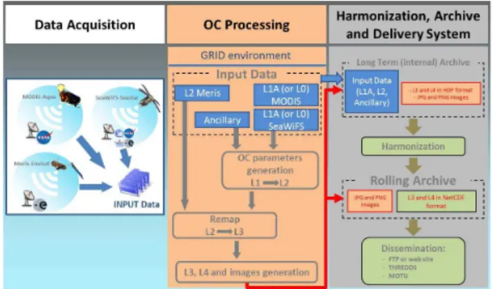
The architecture of the GOS OCOS is based on three main modules: (1) data capture and acquisition facility, (2) the processing system, and (3) the data output harmonization, archive and dissemination. These modules have correspon-dence with the three main functions described in the fol-lowing sections and summarized in Fig. 1. The system is based on a grid computing system with a modular design composed of three separate processing chains (SeaWiFS, MODIS and MERIS) to facilitate maintenance and software upgrades. Moreover, the modular design allows for new sen-sors/satellites to be part of the system without the need of revising the entire system architecture.

The processing module (Fig. 1, middle panel) is the in-terface between input data from space agencies ground seg-ments (NASA and ESA, Fig. 1, left panel) and the data archives and dissemination system (Fig. 1, right panel). This processing module consists of a set of shell scripts, Inter-active Data Language (IDL v8.0, http://www.exelisvis.com/) and SeaWiFS Data Analysis System (SeaDAS v6.1, http: //oceancolor.gsfc.nasa.gov/seadas/) procedures developed by GOS.

Fig. 1.GOS OC system architecture based on three main mod-ules: data capture and acquisition facility from space agency ground segments (left panel); processing system (middle panel); data har-monization, archive and dissemination module (right panel). Blue blocks with white labels show the input data stored into the GOS in-ternal archive. Arrows, blocks and labels marked in red (right panel) display the output products stored within both the GOS internal and rolling archives.

The system operates in two modes: “operational mode” and “on-demand mode”. Operational mode works in near real-time (NRT) or in delayed time (DT):

– NRT is meant to provide users with products as soon as possible. Data are produced once a day, using climato-logical auxiliary data (meteoroclimato-logical and ozone data). Products are made available to the users within 6 or 7 hours after satellite overpass. NRT data are meant for coastal application, water quality monitoring, fishery, and to support in situ data sampling strategy (oceano-graphic cruises);

– DT products are generated when consolidated auxiliary data are available. In general, products are made avail-able to the users 4 or 5 days after satellite overpass. DT products are higher quality than NRT and thus are more suited for data assimilation and validation of ecosys-tem models and to produce value-added products (e.g., phytoplankton primary production). If, for any reason, the auxiliary data needed for the production of the DT data are not available from space agencies at the time of scheduled processing, the associated input data flow is put into a waiting queue until the auxiliary data are made available.

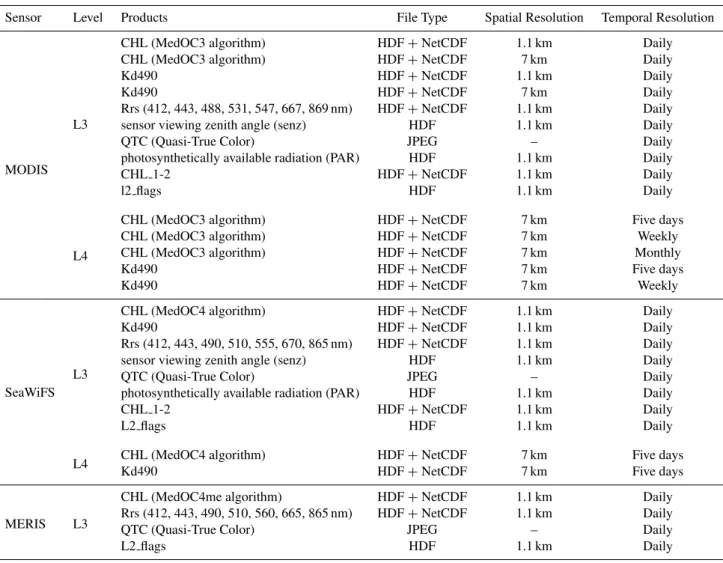
Table 1.OCOS products list routinely generated at GOS. For each product the sensor (MODIS, SeaWiFS or MERIS) is specified, along with the processing level, the data file format, and space-time data resolution.

Sensor Level Products File Type Spatial Resolution Temporal Resolution

MODIS L3

CHL (MedOC3 algorithm) HDF+NetCDF 1.1 km Daily CHL (MedOC3 algorithm) HDF+NetCDF 7 km Daily Kd490 HDF+NetCDF 1.1 km Daily

Kd490 HDF+NetCDF 7 km Daily

Rrs (412, 443, 488, 531, 547, 667, 869 nm) HDF+NetCDF 1.1 km Daily sensor viewing zenith angle (senz) HDF 1.1 km Daily QTC (Quasi-True Color) JPEG – Daily photosynthetically available radiation (PAR) HDF 1.1 km Daily CHL 1-2 HDF+NetCDF 1.1 km Daily

l2 flags HDF 1.1 km Daily

L4

CHL (MedOC3 algorithm) HDF+NetCDF 7 km Five days CHL (MedOC3 algorithm) HDF+NetCDF 7 km Weekly CHL (MedOC3 algorithm) HDF+NetCDF 7 km Monthly Kd490 HDF+NetCDF 7 km Five days Kd490 HDF+NetCDF 7 km Weekly

SeaWiFS L3

CHL (MedOC4 algorithm) HDF+NetCDF 1.1 km Daily Kd490 HDF+NetCDF 1.1 km Daily Rrs (412, 443, 490, 510, 555, 670, 865 nm) HDF+NetCDF 1.1 km Daily sensor viewing zenith angle (senz) HDF 1.1 km Daily QTC (Quasi-True Color) JPEG – Daily photosynthetically available radiation (PAR) HDF 1.1 km Daily CHL 1-2 HDF+NetCDF 1.1 km Daily

L2 flags HDF 1.1 km Daily

L4 CHL (MedOC4 algorithm) HDF+NetCDF 7 km Five days Kd490 HDF+NetCDF 7 km Five days

MERIS L3

CHL (MedOC4me algorithm) HDF+NetCDF 1.1 km Daily Rrs (412, 443, 490, 510, 560, 665, 865 nm) HDF+NetCDF 1.1 km Daily QTC (Quasi-True Color) JPEG – Daily

L2 flags HDF 1.1 km Daily

re-processing scheduling (such as the NASA reprocessing of 2009, 2010, 2012).

2.1 The input data and acquisition facility

The satellite data inputs to the GOS OCOS are the Level 1 (raw data formatted, L1A) or Level 0 (raw spacecraft data, L0) SeaWiFS, L1A (or L0) MODIS-Aqua and Level 2 (de-rived geophysical parameters, L2) MERIS passes covering the MED and BLS domain.

Historically, SeaWiFS L0 data were acquired locally by GOS receiving station (HROM). This station was operational from the SeaWiFS launch in 1997 until the end of iFS mission (at the end of 2010), and was the only SeaW-iFS real-time receiving station with the complete coverage of the MED area, among the 9 other NASA authorized stations worldwide. For operational purposes, during the last years of SeaWiFS mission, GOS SeaWiFS data have been also ac-quired from the European Space Agency rolling archive.

MODIS L1A (or L0) data are acquired automatically from the Goddard Space Flight Center at NASA, via FTP, from a remote directory where all passes covering the MED and BLS domains are stored. MERIS L2 data are acquired from ESA rolling archive. All passes covering the MED and BLS domains are extracted on the base of orbit and track numbers. Consolidated ancillary data (ozone, and, for MODIS only, attitude and ephemerides data) and meteorological data (wind, atmospheric pressure, rain waters, etc.), both for the SeaWiFS and MODIS L1 to L2 DT processing (see Sect. 2.2), are downloaded from NASA and from the Na-tional Centers for Environmental Prediction (NCEP), respec-tively. During this processing step, the knowledge of the ozone concentration distribution is also required and ob-tained via TOAST (Total Ozone Analysis using SBUV/2 and TOVS).

2.2 OC processing system

SeaWiFS and MODIS processing chains are designed to pro-cess data from L1A (or L0) to Level 3 (single geophysical parameters, L3) and Level 4 (multi-day and/or multi-sensor products, L4), whereas MERIS processing chain only deals with L2 to L3 and L4 data (Fig. 1). L0 data are processed to L1A, in case L1A data are not directly available from up-stream data sources.

2.2.1 L1A to L2 processor

The first step consists of the extraction, from each L1A data swaths, of the data actually covering the MED and BLS domain. The extracted L1A files are processed us-ing auxiliary data (climatological data in NRT or consol-idated ancillary data in DT) to obtain geophysical param-eters. The main issue related to this step is the applica-tion of the atmospheric correcapplica-tion procedure and of the bio-optical algorithms to retrieve ocean parameters. This pro-cessing step is carried out using Mediterranean regional al-gorithms as described by Volpe et al. (2007) for SeaW-iFS, and by Santoleri et al. (2008) for MODIS Aqua. L1A data are processed up to L2 applying the dark pixel atmo-spheric correction scheme (Siegel et al., 2000). The result of this step is the remote sensing reflectance (Rrs) at differ-ent wavelengths, which are then used as input for the bio-optical algorithm for oceanic products retrievals. Rrs spec-tra are thus used to compute either the case I water CHL using the Mediterranean-adapted and sensor-specific algo-rithms, or the merged case I-case II water CHL using the method developed by D’Alimonte et al. (2003). Moreover, a new interpolated CHL product is routinely produced at re-duced spatial resolution (4 km) using the Data INterpolat-ing Empirical Orthogonal Functions technique (DINEOF; Beckers and Rixen, 2003). Final L2 files contain the dif-fuse attenuation coefficient at 490 nm (Kd490), CHL using Mediterranean-specific algorithms, photosynthetically active radiation (PAR), the merged case I-case II CHL product, the DINEOF-interpolated CHL, and L2 quality flags (McClain et al., 1995), and the Rrs at seven wavelengths (412, 443, 490, 510, 555, 670 and 865 nm for SeaWiFS; 412, 443, 488, 531, 547, 667 and 869 nm for MODIS). Rrs can be used to pro-duce additional marine OC parameters such as the coloured dissolved organic matter (CDOM) and the total suspended matter (TSM).

Within this step quasi true colour (QTC) images of each satellite pass are also created (in JPEG format). QTC is gen-erated by combining the three OC bands that most closely represent red, green and blue (RGB) in the visible spectrum, creating an image that is fairly close to what the human eye and brain would perceive. For MODIS data HDFLook soft-ware is used (http://www-loa.univ-lille1.fr/Hdflook/hdflook gb.html), while, for SeaWiFS and MERIS, ad-hoc IDL and SeaDAS procedures have been created. These data can be

useful for environmental monitoring. For example, SeaWiFS QTC were recently used in the framework of the EU-funded ADIOS project to monitor the occurrence of Saharan dust events in the Mediterranean Sea (Volpe et al., 2009). 2.2.2 L2 to L3/L4 processor

This step is common to MODIS, SeaWiFS and MERIS processing. Here, relevant parameters for each applica-tion/scientific project are extracted and remapped into single-band products over a common equirectangular geographical projection covering the entire MED and BLS domain (27.6– 48.4° N; 9.5° W–43.5° E). This processor contains both cus-tomized and standard procedures. The standard procedure remaps the L2 products at high resolution (1.1 km at nadir). In this step, for MERIS sensor, further actions are conducted. In fact, in order to obtain the chlorophyll concentration, the standard normalized surface reflectances are converted to remote sensing reflectance and used to obtain the regional chlorophyll concentration using the Mediterranean algorithm described by Santoleri et al. (2008).

Once extracted, daily data files are routinely created (Ta-ble 1) applying a set of flags (standard flags) to mask out pixels affected by any problems. These standard flags are

– for SeaWiFS and MODIS: land, cloud or ice contam-ination, atmospheric correction failure, observed radi-ance very high, high sensor view zenith angle, high so-lar zenith angle, very low water-leaving radiance (cloud shadow), derived product algorithm failure, reduced navigation quality, aerosol iterations exceeded max, re-duced derived product quality, atmospheric correction is suspect, bad navigation and pixel rejected by user-defined filter;

– for MERIS: pixel classified as land, pixel classified as cloud and the confidence flag for standard MERIS CHL product (algal 1). This flag rises in case of at-mospheric correction failure, and/or there are difficul-ties with aerosol correction, or in case of uncorrected glint or whitecaps, or for pixels with high turbidity (PCD 1 15).

2.3 Data harmonization, archive and delivery system

L3 and L4 data files are produced in Hierarchical Data For-mat (HDF) and then converted to NetCDF 3.6 (Network Common Data Form), following the Climate and Forecast convention (CF 1.4), INSPIRE, EN-ISO 19115, 19119 and 19139. Within MyOcean OCTAC, a unique data format has been defined to allow the end-users to efficiently access data from different OC data providers.

Outputs are stored into two main archives based on net-work storage systems: a rolling archive with latest products and a long-term archive that holds historical output as well as input data for (faster) reprocessing purposes.

The resulting data archive (DA) is accessible by users through many interfaces: ftp, THREDDS, and MOTU (My-Ocean customized catalogue software). The delivery sys-tem is consistent with the INSPIRE directive. In particular, THREDDS and MOTU interfaces allow end-users to dis-cover, browse, pre-view and download metadata and full or subset products, based on OPeNDap technologies.

2.4 System monitoring and quality controls

All events relative to data acquisition, products generation and conversion are logged for monitoring purposes. In case of anomalies, exceptions are raised to the support operator and service manager.

The alarms received by an operator can be of two types: warnings and errors. Warning alarms inform the operator of non-serious anomalies. A warning could be notified, i.e., for the lack of an optimal ancillary file (required in DT process-ing chain; see Sect. 2.2), or for low product quality detected by the final scientific quality control (see Sect. 3.2). This type of alarm does not terminate the processing, and instead pro-duces lower quality output. Error alarms inform the opera-tor of serious anomalies. An error could be notified, i.e., for the lack of attitude or ephemeris files (essential in MODIS L1A to L2 processing step), or for an input data file cor-rupted. This type of alarms terminates the processing with-out producing final with-outputs. In any case, the system operator checks, until a defined delay, for the availability of missing satellite passes or of ancillary files to eventually re-submit the whole process. In case of serious anomalies that can af-fect the overall data quality or availability, the GOS service manager promptly alerts the users and the MyOcean forecast-ing centres, which assimilate ocean colour products, with the aim of minimizing the impact on the forecasting outcomes.

Final outputs (L3 or L4) are quality checked at two lev-els: analysis of input data and processing quality, and con-sistency of geophysical signal. The first level derives directly from processing information; that is, these controls take into account corrupted input data or the lack of auxiliary data. The second level consists of an extra-module developed in the context of MyOcean and constitutes the subject of sec-tion 3.2.

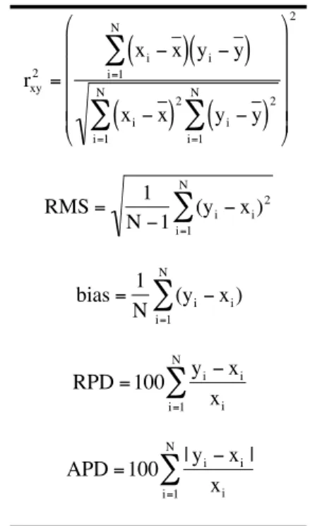
Table 2.Basic statistical quantities used for the assessment of satel-lite (y) data using in situ (x) space-time co-located observations.N

represents the total number of matchup points. The correlation co-efficient (r2) is dimensionless; root mean square (RMS) and bias have the same dimensions as x (in situ observations) and y (satellite measurements). Relative (RPD) and absolute (APD) differences are expressed as percent.

rxy 2 ₌

xi"x

(

)

(

)

N

#

xi"x

(

)

i=1 N

#

(

)

2

i=1 N

#

RMS= 1

N"1 (yi"xi) 2

i=1 N

#

bias= 1

N_i=1(yi"xi

N

#

RPD=100 yi"xi

xi i=1

N

#

APD=100 | yi"xi| xi i=1

N

#

tical quantities used for the assessment of

3 Satellite chlorophyll quality assessment

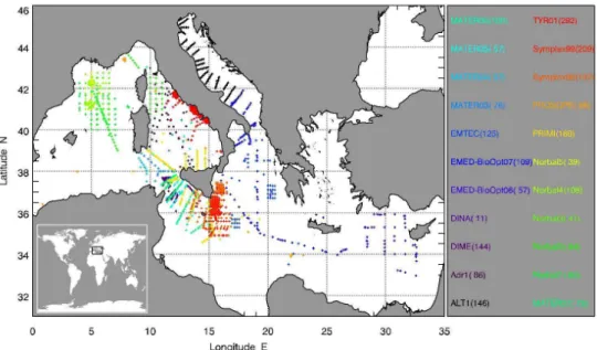
Fig. 2.Location of the in situ CHL dataset. Every cruise is identified by its own colour. For more details about each cruise see Table 3.

3.1 Offline validation

Offline validation refers to the estimate of basic statisti-cal quantities, such as the correlation coefficient (r2), the root mean square (RMS), the bias, and the relative (RPD) and absolute (APD) percentage differences (see Table 2 for details), between single sensor (SeaWiFS, MODIS and MERIS) satellite observations and the corresponding in situ measurements. Given the log-normal CHL distribution,r2, RMS and bias are calculated over log-transformed quanti-ties, while RPD and APD over untransformed pairs of val-ues. In the context of the operational oceanography and of all possible OC data application, two kinds of validation are here performed: one following the NASA standard proto-cols (Mueller and Fargion, 2002) over the current operational product, and another over a daily product for which no flags or masks have been applied (except the cloud mask). The two approaches are hereafter referred to as standard and NoFlags, respectively. In the former case, the analysis relies on the sin-gle sensor flagging system, thus considering all available ob-servations at the best of their scientific reliability; the oppo-site is true for the latter approach.

Single satellite measurements used in the matchup exer-cise are the average of all meaningful pixels within a 3×₃

box centred over the corresponding in situ measurement. From the temporal point of view, all in situ measurements in correspondence with the satellite overpass are considered. When multiple in situ stations fall within the same satellite pixel, their average is taken for the analysis.

3.1.1 In situ dataset

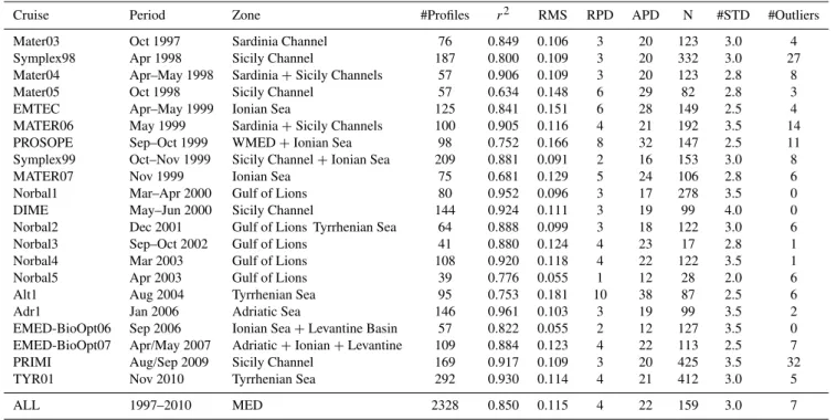
Table 3.List of cruises carried out in the Mediterranean Sea from 1997 to 2010. For each cruise, the total number of calibrated-CHL profiles is reported along with the basic statistics associated with the calibration analysis (see text for details). N represents the total number of bottle-derived fluorescence and HPLC-derived CHL pairs. The number of standard deviation (STD) for the iteratively outlier removal is also indicated. Data from DINA permanent station in the Gulf of Naples, Italy (11 profiles from March to August 2001), are not included in the table as no calibration activity was performed. PROSOPE data were downloaded from http://seabass.gsfc.nasa.gov/seabasscgi/archive index. cgi/NASA GSFC/french. The last row gives the total number of profiles and the average basic statistics. See also Fig. 2.

Cruise Period Zone #Profiles r2 RMS RPD APD N #STD #Outliers

Mater03 Oct 1997 Sardinia Channel 76 0.849 0.106 3 20 123 3.0 4

Symplex98 Apr 1998 Sicily Channel 187 0.800 0.109 3 20 332 3.0 27

Mater04 Apr–May 1998 Sardinia+Sicily Channels 57 0.906 0.109 3 20 123 2.8 8

Mater05 Oct 1998 Sicily Channel 57 0.634 0.148 6 29 82 2.8 3

EMTEC Apr–May 1999 Ionian Sea 125 0.841 0.151 6 28 149 2.5 4

MATER06 May 1999 Sardinia+Sicily Channels 100 0.905 0.116 4 21 192 3.5 14

PROSOPE Sep–Oct 1999 WMED+Ionian Sea 98 0.752 0.166 8 32 147 2.5 11

Symplex99 Oct–Nov 1999 Sicily Channel+Ionian Sea 209 0.881 0.091 2 16 153 3.0 8

MATER07 Nov 1999 Ionian Sea 75 0.681 0.129 5 24 106 2.8 6

Norbal1 Mar–Apr 2000 Gulf of Lions 80 0.952 0.096 3 17 278 3.5 0

DIME May–Jun 2000 Sicily Channel 144 0.924 0.111 3 19 99 4.0 0

Norbal2 Dec 2001 Gulf of Lions Tyrrhenian Sea 64 0.888 0.099 3 18 122 3.0 6

Norbal3 Sep–Oct 2002 Gulf of Lions 41 0.880 0.124 4 23 17 2.8 1

Norbal4 Mar 2003 Gulf of Lions 108 0.920 0.118 4 22 122 3.5 1

Norbal5 Apr 2003 Gulf of Lions 39 0.776 0.055 1 12 28 2.0 6

Alt1 Aug 2004 Tyrrhenian Sea 95 0.753 0.181 10 38 87 2.5 6

Adr1 Jan 2006 Adriatic Sea 146 0.961 0.103 3 19 99 3.5 2

EMED-BioOpt06 Sep 2006 Ionian Sea+Levantine Basin 57 0.822 0.055 2 12 127 3.5 0

EMED-BioOpt07 Apr/May 2007 Adriatic+Ionian+Levantine 109 0.884 0.123 4 22 113 2.5 7

PRIMI Aug/Sep 2009 Sicily Channel 169 0.917 0.109 3 20 425 3.5 32

TYR01 Nov 2010 Tyrrhenian Sea 292 0.930 0.114 4 21 412 3.0 5

ALL 1997–2010 MED 2328 0.850 0.115 4 22 159 3.0 7

that often the sea state does not allow for the water column to be sampled up to the top meter, which mostly contributes to the satellite signal. To overcome this problem, a first eval-uation of the OWP is performed using the single CHL pro-file as it is. The computed OWP is then used to interpolate the CHL profile up to the surface. This new CHL profile is again used to re-compute OWP, which is then used in the matchup exercise. This entire procedure brought an improve-ment of the in situ dataset of about 7 % (APD and 4 % RPD), or 0.02 mg m−3in terms of bias (and with the RMS = 0.06), with respect to Ins2007 used by Volpe et al. (2007) for the validation of the MedOC4 algorithm (see last row in Table 6).

3.1.2 Offline validation results

Main results are summarized in Fig. 3 and Table 4. There is an overall good agreement between satellite-derived CHL and in situ OWP. This work presents the first validation ex-ercise performed over MODIS and MERIS Mediterranean-adapted algorithms in the basin. Despite the lower number of observations, MERIS statistics perform slightly better than those of MODIS (Table 4); both sensors, however, underes-timate in situ OWP. Panels in Fig. 3 show that this under-estimation is particularly evident, for MODIS, in correspon-dence with OWP values lower than 1 mg m−3, while larger

Fig. 3. Scatter plots of the in situ OWP(x-axis) versus the stan-dard satellite-derived operational CHL observations. Left, middle and right panels represent SeaWiFS, MODIS and MERIS, respec-tively. Relevant statistics is shown in Table 4.

values do agree quite well; on the other hand, MERIS under-estimation is concerned with the entire CHL range of vari-ability.

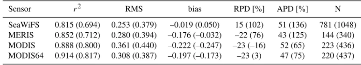
Table 4.Statistical results from the offline validation analysis. Numbers in and outside the brackets refer to the matchup statistics derived with NoFlags and standard approaches described in Sect. 3.1. Last row statistics refer to MODIS matchup file derived using SeaDAS version 6.4.

Sensor r2 RMS bias RPD [%] APD [%] N SeaWiFS 0.815 (0.694) 0.253 (0.379) –0.019 (0.050) 15 (102) 51 (136) 781 (1048) MERIS 0.852 (0.712) 0.280 (0.394) –0.176 (–0.032) –22 (76) 43 (125) 144 (340) MODIS 0.888 (0.800) 0.361 (0.440) –0.222 (–0.247) –23 (–16) 52 (65) 223 (436) MODIS64 0.914 (0.817) 0.308 (0.387) –0.197 (–0.173) –23 (3) 47 (75) 220 (437)

Table 5.Basic statistical quantities as obtained using both the cur-rent operational SeaDAS version (6.1) and the version 4.8 for Sea-WiFS. First row shows the statistics as provided in Table 4 of Volpe et al. (2007); for consistency, r2, RMS and bias are calculated over log-transformed pairs of data. Only stations used by Volpe et al. (2007) are used for this cross-comparison. Second and third rows show the same statistics for all pairs of values, in which both the current (6.1) and the former (4.8) matchup datasets present valid data.

SeaDAS Version r2 RMS bias RPD APD N

4.8 (Volpe et al., 2007) 0.875 0.221 –0.041 3 40 440 4.8 0.884 0.223 –0.041 4 41 360 6.1 0.871 0.244 –0.044 9 48 360

Table 6.Cross-comparison between two SeaWiFS-OWP matchup datasets: the current and the one performed by Volpe et al. (2007). First row shows the comparison between the new in situ dataset (Ins2012) and the SeaWiFS CHL derived using SeaDAS v4.8 (Sat48). Second row refers to SeaDAS v6.1 (Sat61) against the Volpe’s in situ data (Ins2007). Third and fourth rows show the difference between the two SeaDAS versions and the two in situ datasets, respectively.

r2 RMS bias RPD APD N

Sat48 vs. Ins2012 0.889 0.224 –0.057 0 39 360 Sat61 vs. Ins2007 0.861 0.250 0.028 17 54 360 Sat61 vs. Sat48 0.968 0.127 0.013 8 22 360 Ins2012 vs. Ins2007 0.993 0.057 0.016 4 7 360

(3 % RPD and 40 % APD as obtained by Volpe et al., 2007; and reported in Table 5). Since in Volpe et al. (2007) the cor-relation coefficient, the RMS and the bias were calculated over untransformed pairs of values, these statistics have been here recalculated, for consistency, by log-transforming in situ and SeaWiFS-derived CHL using the same dataset (Table 5). The issues that must be taken into account when compar-ing these results with those previously obtained by Volpe et al. (2007) are the different in situ datasets used as refer-ence within the two analyses (see Sect. 3.1.1); the different SeaDAS software configurations within versions 4.8 and 6.1 (for a complete view of the changes occurred within SeaDAS version 6.1, which in turn prompted for the entire NASA sup-ported OC mission reprocessing, visit http://oceancolor.gsfc.

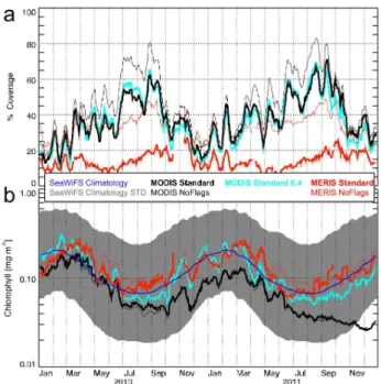
Fig. 4.MODIS and MERIS 2010–2011 time series; (a)the per-centages of good pixels with respect to all sea pixels for both standard(thin) and NoFlags(bold) daily data are marked in red for MERIS and in black for MODIS;(b) average daily chlorophyll concentration for standard(thin), NoFlags(bold) and SeaWiFS cli-matology(blue). The grey area identifies the±one climatological STD with respect to daily average SeaWiFS climatology. For de-tails about climatology, see Sect. 3.2.

Since MODIS sensor calibration has relied, for the overlap-ping period, on the SeaWiFS system, this may have had im-portant implications. Indeed, the last row of Table 4 shows the statistics about MODIS matchup file derived using the latest available version of SeaDAS, the 6.4 version. The com-parison of the last two rows in Table 4 provides a first-order insight of the system calibration impact over the MODIS data quality, in the Mediterranean Sea, resulting in a 5 % APD improvement. This issue will be further explored in the next section.

There are applications, such as OC data assimilation into ecosystem modelling, for which the assessment and maxi-mization of data quality, with respect to the amount of in-formation provided by the single satellite daily image, are crucial, and this is the kind of applications the above anal-ysis refers to. On the contrary, it might be useful to keep as much pixels as possible regardless of their relative sci-entific quality and reliability and depending on the type of application that satellite data are meant to support. An ex-ample can be that of using OC data to guide and support in situ ship-based sampling. In this context, the NoFlags statis-tics generally, but not always, worsen as compared to the standard one (see values in brackets in Table 4). Neverthe-less, the number of available pixels can significantly increase (Fig. 4a; compare also numbers in and outside brackets in

Fig. 5. Statistical occurrence of the L2 flags within NoFlags matchup files for SeaWiFS (left), MODIS (middle) and MERIS (right), whose statistics are shown in brackets in Table 4. Ver-tical dashed lines indicate the flags operationally activated for the standard processing. For a complete description of the phys-ical meaning of the flag bit numbers, the reader should refer to http://oceancolor.gsfc.nasa.gov/VALIDATION/flags.html for Sea-WiFS and MODIS, and to http://earth.eo.esa.int/pcs/envisat/meris/ documentation/meris 3rd reproc/Vol11 Meris 6a.pdf for MERIS.

correspondence with N in Table 4), thus supporting applica-tions just needing qualitative information about the sea sur-face state (e.g., presence/absence of fronts, meanders, or river plumes). However, despite the fact that NoFlags CHL values present higher standard deviation (ca. 20 % to 50 % more for MODIS and MERIS, respectively) than those derived from the standard processing, the resulting basin-scale averages of the log-transformed time series do not significantly dif-fer over monthly to seasonal time scales (compare bold and thin lines in Fig. 4b). To better picture the influence of the single L2 processing flag over the NoFlags analysis, Fig. 5 shows their statistical occurrence for all of the three sen-sors’ matchup files. To conclude, from an operational point of view, the best choice would be to provide the end-users with the most comprehensive information by supplying both CHL and the l2 flags on a daily basis into a single data file.

3.2 Online validation

The aim of the online validation is to assess the temporal consistency of current day satellite observations through the use of both previous day data and of the current day clima-tological satellite data. Satellite climatology is the CNR Sea-WiFS daily CHL climatology, which has been produced with SeaDAS 6.1, using the MedOC4 regional algorithm (Volpe et al., 2007) with a nominal spatial resolution of 4 km. These climatology maps have been created using the data falling into a moving temporal window of ±5 days. One of the main purposes of a climatology field is to serve as reference, and as such it is expected to be as reliable as possible, thus avoid-ing biases caused by savoid-ingle incorrect pixel values. To over-come these possible biases, a filtering procedure has been applied to the entire SeaWiFS time series, by removing all isolated pixels and by filling in all isolated missing pixels us-ing the near-neighbour approach. The resultus-ing climatology time series includes the daily climatological standard devia-tion (STD) on a pixel-by-pixel basis.

The current day data temporal consistency is evaluated in two successive steps:

1. checking, on a pixel-by-pixel basis, whether the differ-ence between the current day observation and that of the previous day falls within or outside four climatological STD. These pixels fall in the statistics named “IN/OUT PrevDay”;

2. In case previous day data do not cover all of the current day pixels, the difference between these current day pix-els and the corresponding current day SeaWiFS tology is computed and compared against four clima-tological STD. These pixels fall in the statistics named “IN/OUT Clima”.

All pixels for which neither the first nor the second approach can be applied are marked as “Missing”. Four STD have been chosen because there can be pretty high variability from one day to the another on a pixel-by-pixel basis, and also because the reference climatology varies much more smoothly than the daily fields.

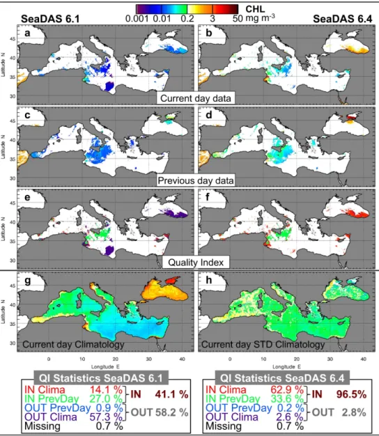
Current day data (1 km) are sub-sampled to 4 km spatial resolution to match the climatology resolution. Here, only results from MODIS Aqua and MERIS are shown, as SeaW-iFS stopped operating on the 11th of December 2010. Fig-ure 6 shows a graphical example of the online validation and refers to the MODIS DT CHL image acquired on the 13th of December, 2011 (Fig. 6a). With the current processing software configuration, which uses SeaDAS 6.1, as much as 46 % of the good pixels fall outside 4 climatological STD (Fig. 6h) as compared to both previous day data (2 % ca., Fig. 6c) or current day climatology (44 %, Fig. 6e). In gen-eral this does not necessarily mean that these pixels present a greater uncertainty level but could suggest the presence of frontal, gyre-induced phytoplankton biomass variability,

Fig. 6.Example of the online validation analysis over MODIS CHL image of the 13th December 2011. Panels(a–c–e)refer to the analysis performed using the current version of SeaDAS software (6.1), and are the daily MODIS DT CHL image, the previous day image, and the quality index, respectively. Panels(d–b–f)refer to the analysis performed using the latest version of SeaDAS software (6.4), and are the daily MODIS DT CHL image, the previous day image, and the quality index, respectively. Panels(g–h)represent the current day climatology and the current day STD climatology, respectively. Apart from panels(e–f), whose colour legend is shown as QI statistics, all units are in mg m−3and refer to the colour bar. Numbers in the QI statistics are normalized to the total number of good pixels within the current day image, which are 15 227 and 12 315, respectively for SeaDAS 6.1 and SeaDAS 6.4.

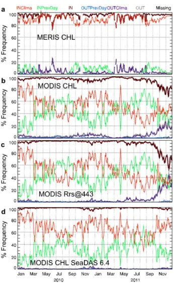
partially unsolved. The point here is that pixels marked as OUT Clima (Fig. 6e) in the Ionian Sea are masked out in the L2 to L3 standard processing (SeaDAS 6.4) because of the very low water-leaving radiance (Flag Bit Number = 15), and thus do not concur to generate the QI statistics. On the con-trary, pixels in the Black Sea that are marked as OUT Clima within the SeaDAS 6.1 processing have been successfully re-covered by the new calibration scheme, thus belonging to the IN Clima pixels.

Fig. 7.Online validation statistics time series for the 2010–2011 time period, for(a)MERIS CHL,(b)MODIS CHL,(c)MODIS Rrs at 443 nm processed using the current version of SeaDAS software (6.1), and(d)MODIS CHL processed using the latest available ver-sion of SeaDAS software (6.4). Colour legend refers to definition provided in Sect. 3.2 and graphically shown in Fig. 6. In addition, the total percentages of pixels falling in and outside relevant criteria are marked in dark red and grey, respectively. All lines represent the moving averages using a five-day interval.

contiguous swath overlap is quite frequent, and this is shown by the opposition-of-phase of the IN PrevDay and the IN Clima number of pixels (green and red lines in Fig. 7b), which in turn points to the cloudiness annual cycle, with a good overlap during summer. The most important outcome of this analysis is that our method efficiently captured the timing of MODIS bands degradation and, more importantly, that the new SeaDAS version was able to address it success-fully.

4 Conclusions

In this work we have described the major scientific and tech-nological steps made to develop, maintain and improve the Mediterranean Ocean Colour Observing System, from the data upstream providers to the product quality assessment. The system is made of three modules: (1) data capture and acquisition facility; (2) the processing system; (3) and the data output harmonization, archive and dissemination. Each of these modules is automatically checked for performance quality; the outcome of this continuous process is a quality log into which all necessary information for solving the pos-sible problems that can arise within each of the processing steps is stored. There are thus two kinds of quality assess-ments, of which one is purely technical and refers to the sys-tem itself, and the other is from a scientific point of view. The former has been described, and the error and warning alerts have demonstrated to be very efficient to track uncer-tainties back to their sources and causes. The ultimate goal of this quality assessment is to timely alert the users with special attention to other operationally data providers that use GOS-product as upstream data sources for their services. As for the latter, two distinct validation processes are per-formed within GOS OCOS: the online and the offline vali-dations. The offline validation refers to the product quality assessment performed via the in situ data comparison, and is performed every time a significant change in the processing chain takes place, e.g., in case of an algorithm update. The present analysis relies on the most up-to-date in situ CHL dataset for the Mediterranean Sea, whose quality has been improved through a careful analysis of the single CHL pro-files. Main results highlight the SeaWiFS product to be the most reliable in terms of basic statistical quantities, while MODIS- and MERIS-derived products do show a slight but systematic underestimation of the in situ field. This analysis showed that there has been a slightly worse SeaWiFS perfor-mance as compared to previous results. The two most plau-sible causes have been identified: the processing software and the sensor degradation with time. As for the former, de-spite the evidence for the improvement of the CHL retrieval at global scale with SeaDAS 6.1, our analysis demonstrates that the CHL retrieval remains below the quality target ex-pectations in the Mediterranean Sea. Moreover, there is also evidence of a drift in the SeaWiFS signal that has not fully been corrected by the vicarious calibration meant to prevent the signal degradation with time. This issue should be prop-erly addressed by space agencies if a full exploitability of the amazingly valuable SeaWiFS mission has to be accom-plished.

series, is that MODIS-derived chlorophyll exhibits, starting from mid-2010, a severe drift towards the low end of its range of variability. This drift depends in turn on the degradation of the channel at 443 nm. This system can thus be used to inform both the end-users and the upstream data providers about the quality of the product and of the data sources, re-spectively. A new SeaDAS release was recently issued with a new calibration scheme. This new SeaDAS version has demonstrated to successfully address the MODIS calibra-tion issues in the Mediterranean and Black Sea. Based on these results, GOS OCOS has implemented, since June 2012, SeaDAS 6.4 in its operational processing chains to provide users with state-of-the-art products with outstanding scien-tific quality as fully demonstrated in this work.

Acknowledgements. This work was supported by grants from the EU GMES MyOcean project. None of this work could have been possible without the amazing job done by the Ocean Biology and Processing Group and the SeaDAS Development Group from NASA for assessing the MODIS Aqua calibration issues and for making available the updated SeaDAS version. All in situ observations presented in this work were collected by the Italian National Research Council and the Stazione Zoologica “Anthon Dorhn” in the framework of several national projects funded by the Italian Space Agency. Stazione Zoologica “Anthon Dorhn” is acknowledged for the chemical analysis of in situ samples. Authors thank two anonymous reviewers for their constructive comments. Edited by: A. Schiller

References

Bailey, S. W., McClain, C. R., Werdell, P. J., and Schieber, B. D.: Normalized water-leaving radiance and chlorophyll a match-up analysis, SeaWiFS Postlaunch Calibration and Validation Anal-yses, Part 2, NASA Goddard Space Flight Center, Greenbelt, Maryland, NASA Tech. Memo. 1999–206892, Vol. 10, 2000. Bailey, S. W. and Werdell, P. J.: A multi-sensor approach for the

on-orbit validation of ocean color satellite data products, Remote Sens. Environ., 102, 12–23, 2006.

Beckers, J. M. and Rixen, M.: EOF calculations and data filling from incomplete oceanographic datasets, J. Atmos. Ocean. Tech., 20, 1839–1856, 2003.

Bricaud, A., Bosc, E., and Antoine, D.: Algal biomass and sea sur-face temperature in the Mediterranean Basin – Intercomparison of data from various satellite sensors, and implications for pri-mary production estimates, Remote Sens. Environ., 81, 163–178, 2002.

Claustre, H., Morel, A., Hooker, S. B., Babin, M., Antoine, D., Oubelkheir, K., Bricaud, A., Leblanc, K., Queguiner, B., and Maritorena, S.: Is desert dust making oligotrophic waters greener?, Geophys. Res. Lett., 29, 1469, 2002.

D’Alimonte, D., Melin, F., Zibordi, G., and Berthon, J. F.: Use of the Novelty Detection Technique to Identify the Range of Ap-plicability of Empirical Ocean Color Algorithms, IEEE Trans. Geosci. Remote Sensing, 41, 2833–2843, 2003.

D’Ortenzio, F., Marullo, S., Ragni, M., d’Alcala, M. R., and Santoleri, R.: Validation of empirical SeaWiFS algorithms for chlorophyll- alpha retrieval in the Mediterranean Sea - A case study for oligotrophic seas, Remote Sens. Environ., 82, 79-94, 2002.

Darecki, M. and Stramski, D.: An evaluation of MODIS and SeaW-iFS bio-optical algorithms in the Baltic Sea, Remote Sens. Envi-ron., 89, 326–350, 2004.

Gregg, W. W. and Casey, N. W.: Global and regional evaluation of the SeaWiFS chlorophyll data set, Remote Sens. Environ., 93, 463–479, 2004.

Hooker, S. B. and McClain, C.: The calibration and validation of SeaWiFS data, Prog. Oceanogr., 45, 427–465, 2000.

Kahru, M. and Mitchell, B. G.: Blending of ocean colour algorithms applied to the Southern Ocean, Remote Sens. Lett., 1, 119-124, 2010.

Lazzari, P., Teruzzi, A., Salon, S., Campagna, S., Calonaci, C., Colella, S., Tonani, M., and Crise, A.: Pre-operational short-term forecasts for Mediterranean Sea biogeochemistry, Ocean Sci., 6, 25–39, doi:10.5194/os-6-25-2010, 2010.

Le Traon, P. Y.: Satellites and Operational Oceanography, in: Op-erational Oceanography in the 21st Century, edited by: Schiller, A., and Brassington, G., Springer Dordrecht Heidelberg London New York, 29–54, 2011.

McClain, C. R., Arrigo, K. R., Esaias, W., Darzi, M., Patt, F. S., Evans, R. H., Brown, C. W., Brown, J. W., Barnes, R. A., and Ku-mar, L.: SeaWiFS Quality Control Masks and Flags: Initial Algo-rithms and Implementation Strategy, SeaWiFS Technical Report Series, SeaWiFS Algorithms, Part 1, Vol. 28, edited by: Hooker, S. B., Firestone, E. R., and Acker, J. G., NASA Goddard Space Flight Center, Greenbelt, Maryland, 3–7, 1995.

Mueller, J. L. and Austin, R. W.: Ocean Optics Protocols for Sea-WiFS Validation, Revision 1., NASA Tech. Memo. 104566, Vol. 25, edited by: Hooker, S. B., Firestone, E. R., and Acker, J. G., NASA Goddard Space Flight Center, Greenbelt, Maryland, 67 pp, 1995.

Mueller, J. L. and Fargion, G. S.: Ocean Optics Protocols for Satellite Ocean Color Sensor Validation, Revision 3. NASA Tech. Memo. 2002–210004, NASA Goddard Space Flight Cen-ter, Greenbelt, Maryland, 308 pp, 2002.

Natvik, L.-J. and Evensen, G.: Assimilation of ocean colour data into a biochemical model of the North Atlantic Part 1. Data as-similation experiments, J. Mar. Syst., 40–41, 127–153, 2003. O’Reilly, J. E., Maritorena, S., Mitchell, B. G., Siegel, D. A.,

Carder, K. L., Garver, S. A., Kahru, M., and McClain, C.: Ocean color chlorophyll algorithms for SeaWiFS, J. Geophys. Res.-Oceans, 103, 24937–24953, 1998.

O’Reilly, J. E., Maritorena, S., Siegel, D., O’Brien, M. C., Toole, D., Mitchell, B. G., Kahru, M., Chavez, F. P., Strutton, P., Cota, G., Hooker, S. B., McClain, C. R., Carder, K. L., Muller-Karger, F., Harding, L., Magnuson, A., Phinney, D., Moore, G. F., Aiken, J., Arrigo, K. R., Letelier, R., and Culver, M.: Ocean color chloro-phyll a algorithms for SeaWiFS, OC2, and OC4: version 4., in: SeaWiFS Postlaunch Technical Report Series, vol.11. SeaWiFS postlaunch calibration and validation analyses: part 3, edited by: Hooker, S. B. and Firestone, E. R., NASA Goddard Space Flight Center., Greenbelt, MD:, 9–23, 2000.

in: Remote Sensing of the European Seas, edited by: Barale, V. and Gade, M., Springer, 103–116, 2008.

Siegel, D. A., Wang, M., Maritorena, S., and Robinson, W.: At-mospheric correction of satellite ocean color imagery: the black pixel assumption, Appl. Opt., 39, 3582–3591, 2000.

Triantafyllou, G., Korres, G., Hoteit, I., Petihakis, G., and Banks, A. C.: Assimilation of ocean colour data into a Biogeochemical Flux Model of the Eastern Mediterranean Sea, Ocean Sci., 3, 397–410, doi:10.5194/os-3-397-2007, 2007.

Volpe, G., Santoleri, R., Vellucci, V., Ribera d’Alcala, M., Marullo, S., and D’Ortenzio, F.: The colour of the Mediterranean Sea: Global versus regional bio-optical algorithms evaluation and im-plication for satellite chlorophyll estimates, Remote Sens. Envi-ron., 107, 625–638, 2007.

Volpe, G., Banzon, V. F., Evans, R., Santoleri, R., Mariano, A. J., and Sciarra, R.: Satellite observations of the impact of dust in a low nutrient low chlorophyll region: fertiliza-tion or artefact?, Glob. Biogeochem. Cycle, 23, GB3007, doi:3010.1029/2008GB003216, 2009.