ESTIMATES OF SOLUTIONS
FOR PARABOLIC DIFFERENTIAL
AND DIFFERENCE FUNCTIONAL EQUATIONS
AND APPLICATIONS
Lucjan Sapa
Abstract. The theorems on the estimates of solutions for nonlinear second-order partial differential functional equations of parabolic type with Dirichlet’s condition and for suitable implicit finite difference functional schemes are proved. The proofs are based on the com-parison technique. The convergent and stable difference method is considered without the assumption of the global generalized Perron condition posed on the functional variable but with the local one only. It is a consequence of our estimates theorems. In particular, these results cover quasi-linear equations. However, such equations are also treated separately. The functional dependence is of the Volterra type.
Keywords: parabolic differential and discrete functional equations, estimate of solution, implicit difference method.
Mathematics Subject Classification:35R10, 35B30, 65M12, 65M06.
1. INTRODUCTION
The aim of the paper is to prove theorems on the estimates of solutions for non-linear second-order partial differential functional equations of parabolic type with Dirichlet’s condition and for generated by them implicit finite difference functional schemes. We also give the applications of the results. More precisely, we prove the theorem on the convergence of a difference method to a classical solution for the differential functional problem, which by the given estimates, may be treated in the subspaceC(Ω, R)⊂C(Ω,R), where R⊂Ris an interval. It is a new idea in area of
nonlinear implicit difference methods which was studied for explicit methods by K. Kropielnicka and L. Sapa [14]. This considerably extends the class of problems which are solvable by the described method. Therefore, the Lipschitz, Perron or generalized Perron conditions posed onfwith respect tozneed not be global, inC(Ω,R), as in the papers due to M. Malec, Cz. Mączka, W. Voigt, M. Rosati and L. Sapa [15–19,24,25],
529
Z. Kamont, H. Leszczyński and K. Kropielnicka [9–13], but in C(Ω, R)only. In par-ticular, equations with the polynomial right-hand side are admitted (see the examples in Section 8). Our results can be extended to weakly coupled systems. Let us stress that unlike [14, 25], the Courant-Friedrichs-Levy condition on the steps of a mesh is omitted (see Remark 6.4).
We now formulate the differential functional problem. Let functions f : ∆ → R andϕ:E0∪∂0E→Rbe given (the relevant sets are defined in Section 2.1). Consider
a nonlinear second-order partial differential functional equation of parabolic type of the form
∂tz(t, x) =f(t, x, z, ∂xz(t, x), ∂xxz(t, x)) (1.1)
with theinitial conditionand theboundary condition of the Dirichlet type
z(t, x) =ϕ(t, x) on E0∪∂0E, (1.2)
where ∂xz = (∂x1z, . . . , ∂xnz),∂xxz=
∂xixjz n
i,j=1. The equation may be nonlinear
with respect to second derivatives. Such an equation is called strongly nonlinear. The functional dependence is of the Volterra type (e.g., delays or Volterra type integrals). Let aij : ∆A → R and F : ∆F → R, i, j = 1, . . . , n, be given functions (see
Section 2.1). If we assume that eachaij is non-positive or non-negative in∆A, then
our results, in particular, cover a quasi-linear differential functional equation of the form
∂tz(t, x) = n
X
i,j=1
aij(t, x, z)∂xixjz(t, x) +F(t, x, z, ∂xz(t, x)). (1.3)
To omit this condition, another scheme is also studied.
We assume the existence of a classical solution of problems (1.1), (1.2) and (1.3), (1.2). Theorems on the existence and uniqueness of such solutions for some special parabolic differential functional equations with different boundary conditions can be found in [3–5, 7, 21, 29] and the references therein.
The equation
∂tz(t, x) = n
X
i=1
∂xixia(z(t, x)) +
n
X
i=1
∂xib(z(t, x)) +c(z(t, x)), (1.4)
where a, b, c : R → R are given functions, is a special case of (1.1) and (1.3). In applications, the second-order term on the right-hand side of (1.4) corresponds to a diffusive or dispersive process, the first-order term represents a convective or advective phenomenon, while the last term corresponds to a reactive process, sorption, source or sink. The unknown usually represents a nonnegative biological, medical, physical or chemical variable such as density, saturation or concentration. A lot of equations of type (1.4) with the polynomial right-hand side is described in [1, 6, 8, 20]. It is for example the generalized Fisher equation
∂tz(t, x) =∂x1x1z(t, x) +βz(t, x)
h
n= 1, β∈R,δ >0, and the reaction-diffusion equation
∂tz(t, x) = n
X
i=1
∂xixi(z(t, x))
m−
β(z(t, x))δ, (1.6)
m > 0, δ > 0, β ∈ R (see Examples 8.1, 8.2). Equation (1.5) for β = δ = 1 (the Fisher equation) is the archetypical deterministic model for the spread of an ad-vantageous gene in a population of diploid individuals living in a one-dimensional habitat. Equation (1.6) is a simple and widely used model for various physical, chem-ical and biologchem-ical problems involving diffusion with a source or with absorption, as for instance in modelling filtration in porous media, transport of thermal energy in a plasma, flow of a chemically reacting fluid from a flat surface, evolution of popula-tions, etc. Equations of type (1.4) which can be also covered by our theorems are the Newell-Whitehead equation, the Zeldovich equation, the KPP equation, the Nagumo equation, the Huxley equation and others considered in [6, 20].
The results concerning numerical methods, differential functional and difference functional inequalities or the uniqueness theory, appearing in the papers of P. Besala, G. Paszek [2], C.V. Pao [22], R. Redheffer, W. Walter [23, 28], J. Szarski [26, 27] and numerous others, do not apply to nonlinear equations and quasi-linear equations with such a general functional dependence as in our paper.
The paper is organized in the following way. In Section 2 notation is introduced and some definitions are formulated. Section 3 deals with the estimates of solutions for problems (1.1), (1.2) and (1.3), (1.2). Two next sections are concerned with the estimates of solutions for some auxiliaries discrete functional equations and for im-plicit difference functional schemes generated by problem (1.1), (1.2), respectively. In Section 6 the convergence of the difference method for (1.1), (1.2) is studied. In Section 7 the modified difference method for (1.3), (1.2) is considered. Finally, in the last section examples illustrating our results and numerical experiments are presented.
2. NOTATION AND DEFINITIONS
2.1. SETS AND FUNCTION SPACES, PARABOLICITY
Let T > 0, X = (X1, . . . , Xn), τ0 ≥ 0, τ = (τ1, . . . , τn), where Xi > 0, τi ≥0 for
i= 1, . . . , n, be given. Define
E= [0, T]×(−X, X)⊂R1+n, (2.1)
E0= [−τ0,0]×[−X−τ, X+τ]⊂R1+n,
∂0E= [0, T]×([−X−τ, X+τ]\(−X, X))⊂R1+n.
Let, moreover,
Ω =E∪E0∪∂0E, (2.2)
Denote byMn×n the class of alln×nsymmetric real matrices. Define the sets
∆ =E×C(Ω,R)×Rn×Mn×n, (2.3)
∆A=E×C(Ω,R), ∆F =E×C(Ω,R)×Rn,
∆∗=E×C(Ω, R)×Rn×Mn×n,
∆A∗=E×C(Ω, R), ∆F∗=E×C(Ω, R)×Rn,
whereR⊂Ris a fixed interval andC(Ω, R) ={z: Ω→R} ∩C(Ω,R).
Equation (1.1) is said to be parabolic in Walter’s sense if for any two matrices
q,qe∈Mn×n there is
q≤qe⇒f(t, x, z, p, q)≤f(t, x, z, p,qe)
for(t, x)∈E,z∈C(Ω,R),p∈Rn, where the inequalityq≤eqmeans that the matrix e
q−q is positive defined (see [28, §23]). To adopt this definition to equation (1.3) it is enough to replace the right-hand side of the above implication by the inequality Pn
i,j=1aij(t, x, z) (qij−eqij)≤0.
Themaximum normsinRn andMn×n are denoted byk · k, while in the space of
continuous functionsC(A,R), A⊂Ωa compact subset, byk · kA.
For a fixedt∈[0, T],
kzkΩt = maxz t, xe : et, x∈Ωt (2.4)
is a seminorm inC(Ω,R), where z∈C(Ω,R).
2.2. DISCRETIZATION, DIFFERENCE AND INTERPOLATING OPERATORS
We use vectorial inequalities to mean that the same inequalities hold between the cor-responding components. We writex⋄y= (x1y1, . . . , xnyn)forx= (x1, . . . , xn), y=
(y1, . . . , yn)∈Rn. Define a mesh on the set Ωin the following way. Let(h0, h′) =h,
h′ = (h1, . . . , hn), stand for the steps of the mesh. Denote by H the set of all
h such that there exist N0 ∈ Z and N = (N1, . . . , Nn) ∈ Nn with the
proper-ties: N0h0 = τ0, N ⋄h′ = X +τ. Obviously, H 6= ∅ and there are K0 ∈ N and
K= (K1, . . . , Kn)∈Znsuch thatK0h0≤T <(K0+ 1)h0,K⋄h′ < X≤(K+ 1)⋄h′.
Forh∈H and(µ, m)∈Z1+n,m= (m1, . . . , mn), we define nodal points t(µ), x(m),
x(m)=x(m1)
1 , . . . , x (mn)
n
, in the following way
t(µ)=µh0, x(m)=m⋄h′.
Forh∈H, we put
Rh1+n=nt(µ), x(m): (µ, m)∈Z1+no. (2.5)
Define the discrete sets
E0.h=E0∩R1+h n, ∂0Eh=∂0E∩R1+h n,
Ωh=Eh∪E0.h∪∂0Eh,
Ωh.µ= Ωh∩
h
−τ0, t(µ) i
×Rn, µ= 0, . . . , K0.
Let, moreover,
Eh+=nt(µ), x(m)∈Eh: 0≤µ≤K0−1 o
, (2.7)
Ih=
n
t(µ): 0≤µ≤K0 o
, Ih+=nt(µ): 0≤µ≤K0−1 o
. (2.8)
Writeχ= 1 + 2n2and
Λ ={λ= (λ1, . . . , λn) : λi ∈ {−1,0,1}, i= 1, . . . , n, |λ| ≤2}, (2.9)
Λ′ = Λ\{0},
where|λ|=|λ1|+. . .+|λn|.
Note that χis the number of elements ofΛ. Letψ: Λ→ {1, . . . , χ} be a function such that ψ(λ) 6= ψ λ for λ 6= λ. We assume that ≺ is an order in Λ defined in the following way: λ ≺λ ifψ(λ)≤ ψ λ. Elements of the space Rχ we denote by
ξ = ξ(λ)
λ∈Λ. For a functionz ∈ F(Ωh,R) and a point t
(µ), x(m) ∈ E
h we put
zhµ,mi= z(µ,m+λ)
λ∈Λ.
For a mesh function z : Ωh ⊃ Ah → R and a point t(µ), x(m) ∈ Ah, we put
z(µ,m)=z t(µ), x(m), |z|(µ,m)=|z(µ,m)|. We denote the space of all such functions
byF(Ah,R)and call it thespace of mesh functions. InF(Ah,R), we introduce the
maximum norm
kzkA
h = max n
z(µ,m): t(µ), x(m)∈Ah
o
, (2.10)
where z ∈F(Ah,R). The symbol z|Ah stands for the restriction of z to Ah. Analo-gously,F(Ah, R) ={z:Ah→R} ∩F(Ah,R), where R⊂Ris a fixed interval.
For a fixedµ∈ {0,1, . . . , K0},
kzkΩh.µ = maxnz(eµ,m)
: t(µe), x(m)∈Ωh.µ
o
(2.11)
is a seminorm in the spaceF(Ωh,R), wherez∈F(Ωh,R).
For a function z : Ih ⊃ Ah → R+, we put z(µ) = z t(µ), t(µ) ∈ Ah, where
R+= [0,+∞). Write
Γ ={(i, j) : 1≤i, j≤n, i6=j}
and suppose thatΓ+,Γ−⊂Γare such thatΓ+∪Γ− = Γ,Γ+∩Γ−=∅(in particular, it may happen thatΓ+=∅orΓ−=∅). We assume that(i, j)∈Γ+ when(j, i)∈Γ+
Letz∈F(Ωh,R)and t(µ), x(m)∈Eh. Set
δ+i z(µ,m)= 1
hi
h
z(µ,m+ei)−z(µ,m)i, (2.12)
δ−i z(µ,m)= 1
hi
h
z(µ,m)−z(µ,m−ei)i,
where ei = (0, . . . ,0,1,0, . . . ,0) with 1 in the ith entry,i = 1, . . . , n. We apply the
difference quotientsδ0,δ= (δ1, . . . , δn), δ(2)= [δij]ni,j=1 given by
δ0z(µ,m)= 1
h0 h
z(µ+1,m)−z(µ,m)i, (2.13)
δiz(µ,m)=
1 2
h
δi+z(µ,m)+δi−z(µ,m)i for i= 1, . . . , n,
δiiz(µ,m)=δi+δ
−
i z
(µ,m) for i= 1, . . . , n,
δijz(µ,m)=
1 2
h
δ+i δ−j z(µ,m)+δ−
i δ
+
jz
(µ,m)i for (i, j)∈Γ −,
δijz(µ,m)=
1 2
h
δi+δj+z(µ,m)+δ−i δ−jz(µ,m)i for (i, j)∈Γ+.
We use these operators to approximate derivatives in equations (1.1) and (1.3). We say that an operatorGh:F(Ωh,R)→C(Ω,R)is aninterpolating operatorif
it has the properties:
(1) for allz∈C1,2(Ω,R)
lim
h→0kGh[Z]−zkΩ= 0,
whereZ:=z|Ωh is the restriction ofz toΩh, (2) for allz, z∈F(Ωh,R)
kGh[z]−Gh[z]kΩt(µ) ≤ kz−zkΩh.µ, µ= 0, . . . , K0.
We apply these operators to approximate the functional term in equations (1.1) and (1.3). An example ofGhis the well-known linear operator Th introduced in [10].
3. ESTIMATES OF SOLUTIONS
FOR THE DIFFERENTIAL FUNCTIONAL PROBLEMS
In this section we give a theorem concerning the estimates of solutions for the differ-ential functional problems (1.1), (1.2) and (1.3), (1.2).
We need the following assumptions on the functions f,ϕ.
Assumption H[f, ϕ]
(H1) There is a function σ0 : [0, T]×R+ → R+ for which the following properties
(1) σ0 is continuous;
(2) the maximal solutionωe of the Cauchy problem
ω′(t) =σ0(t, ω(t)), ω(0) =kϕkE0 is defined on [0, T] ; (3.1)
(3) for each(t, x)∈E andz∈C(Ω,R)
|f(t, x, z,0,0)| ≤σ0 t,kzkΩt
. (3.2)
Theorem 3.1. Let Assumption H[f, ϕ] be satisfied and let (1.1)be parabolic. If u∈
C1,2(Ω,R)is a solution of (1.1),(1.2)and
|ϕ(t, x)| ≤ωe(t) on ∂0E, (3.3)
then
|u(t, x)| ≤ωe(t) on Ω, (3.4)
whereωe is the maximal solution of (3.1).
The proof of a more general version of Theorem 3.1 is given in [14]. So called parabolic solutions of (1.1) are considered there.
Remark 3.2. It follows from the monotonicity ofωethat if we putω(0) =kϕkE0∪∂0E in (3.1), then (3.3) holds. But, by the ordinary differential inequalities, the estimate in (3.4) is worse than forω(0) =kϕkE0.
Remark 3.3. Replacing (3.2) by
|F(t, x, z,0)| ≤σ0 t,kzkΩt
(3.5)
we immediately obtain a version of Theorem 3.1 for problem (1.3), (1.2).
4. DISCRETE FUNCTIONAL EQUATIONS
We consider an implicit discrete functional equation of the Volterra type with the initial boundary condition. Next we give two theorems on the existence and uniqueness and on the estimate of a solution of this problem, respectively. They will be applied in the existence, uniqueness and estimate proofs of a solution for the implicit difference functional scheme (5.1) generated by the differential functional problem (1.1), (1.2) in the next section.
Suppose that a functional Fh : Eh+ ×F(Ωh,R) × Rχ → R is given. For
t(µ), x(m), z, ξ∈E+
h ×F(Ωh,R)×Rχ, we writeFh[z, ξ]
(µ,m)
=Fh t(µ), x(m), z, ξ.
Givenϕh∈F(E0.h∪∂0Eh,R), we consider the discrete functional equation
z(µ+1,m)=Fh
z, zhµ+1,mi (µ,m)
(4.1)
with the initial boundary condition
Note that the numbers z(µ+1,m+λ), λ ∈ Λ, appear in z
hµ+1,mi so (4.1), (4.2) is an implicit problem.
We say that the functionalFhsatisfies the Volterra condition if t(µ), x(m)∈Eh+,
ξ∈Rχ,z, z ∈F(Ω
h,R),z|Ωh.µ =z|Ωh.µ, then Fh[z, ξ] (µ,m)
=Fh[z, ξ](µ,m). Observe
that the Volterra condition states that the value ofFh at t(µ), x(m), z, ξdepends on
t(µ), x(m), ξand the restriction of the functionzto the setΩ
h.µonly. However, this
well-known condition does not imply the existence of a solution for (4.1), (4.2) so we give a suitable theorem.
The following assumptions onFh will be needed.
Assumption H[Fh]
(H1) Fh is of the Volterra type,h∈H.
(H2) There exist partial derivatives ∂ξ(λ)Fhλ∈Λ on Eh+ ×F(Ωh,R)×Rχ, and
∂ξ(0)Fh[z,·](µ,m) is bounded for each t(µ), x(m), z∈E+
h ×F(Ωh,R).
(H3) The conditions
∂ξ(λ)Fh[z, ξ](µ,m)≥0, λ∈Λ′, (4.3)
X
λ∈Λ
∂ξ(λ)Fh[z, ξ](µ,m)= 0 (4.4)
are satisfied at each t(µ), x(m), z, ξ∈E+
h ×F(Ωh,R)×Rχ.
Theorem 4.1. If AssumptionH[Fh]is satisfied, then there exists exactly one solution
v∈F(Ωh,R)of problem (4.1),(4.2).
The proof of Theorem 4.1 is given in [24] and is omitted.
Suppose that v ∈ F(Ωh,R) is the solution of (4.1), (4.2). Define me(µ) ∈ Zn,
µ= 0, . . . , K0, as follows
|v|(µ,me(µ))= maxn|v|(µ,m): t(µ), x(m)∈Ωh
o
. (4.5)
Theorem 4.2. Suppose that Assumption H[Fh]is satisfied and
(1) σh :Ih+×R+ → R+ is nondecreasing with respect to the second variable and if
t(µ), x(me(µ+1))∈E+
h, then
Fh
v, vhµ+1,me(µ+1)i
(µ,me(µ+1)) ≤σh
t(µ),kvkΩh.µ, (4.6)
µ= 0, . . . , K0−1, wherev∈F(Ωh,R)is the solution of (4.1),(4.2),
(2) β:Ih→R+ is nondecreasing and satisfies the recurrent inequality
β(µ+1)≥σ
h
t(µ), β(µ), µ= 0, . . . , K
0−1, (4.7)
andβ(0)≥ kϕ
hkE0.h∪∂0Eh.
Then
Proof. We prove assertion (4.8) by induction onµ.
It follows from the initial condition (4.2) that inequality (4.8) is satisfied forµ= 0. Assume (4.8) for a fixed µ, 0 ≤ µ ≤ K0 −1, we prove it for µ + 1. Let
t(µ), x(me(µ+1))∈E+
h. The assumptions of the theorem and the induction assumption
lead to the inequalities
v(µ+1,me(µ+1))
=Fh
v, vhµ+1,me(µ+1)i
(µ,me(µ+1)) ≤
≤σh
t(µ),kvk Ωh.µ
≤σh
t(µ), β(µ)≤ β(µ+1). (4.9)
In the case t(µ), x(me(µ+1))∈∂
0Eh, the boundary condition (4.2) and the
monotonic-ity of β imply
v(µ+1,me(µ+1))≤ kϕhkE0.h∪∂0Eh ≤β
(0)≤β(µ+1). (4.10)
Hence, the proof is complete by induction.
Remark 4.3. Let the assumptions of Theorem 4.2 be satisfied with
σh(t, y) = (1 +Lh0)y, (t, y)∈Ih+×R+,
whereL≥0. Then
kvkΩh.µ ≤(1 +Lh0)µkϕhkE0.h∪∂0Eh≤exp (LT)kϕhkE0.h∪∂0Eh (4.11)
forµ= 0, . . . , K0. These estimates may be obtained by solving the initial comparison
problem (
β(µ+1)= (1 +Lh
0)β(µ), µ= 0, . . . , K0−1,
β(0) =kϕ
hkE0.h∪∂0Eh
(4.12)
(see assumption (2)). Moreover, it follows from the proof of Theorem 4.2 that if
v(µ,m)≤(1 +Lh0)µkϕhkE0.h on ∂0Eh, (4.13)
then, by puttingβ(0)=kϕhkE0.h in (4.12), the normkϕhkE0.h∪∂0Eh in (4.11) can be replaced bykϕhkE0.h and the estimate is better.
Remark 4.4. It follows from the proof of Theorem 4.2 that if we assume (4.6) for any t(µ), x(m)∈E+h andz∈F(Ωh,R)(see Theorem 4.1 in [14]), then Theorem 4.2
will be also true. But such a version will not be useful in the proof of Theorem 5.3.
5. ESTIMATES OF SOLUTIONS
FOR IMPLICIT DIFFERENCE FUNCTIONAL SCHEMES
We define an implicit finite difference functional scheme which will be applied to approximate a classical solution of the differential functional problem (1.1), (1.2). It is the system of algebraic equations
(
δ0z(µ,m)=f t(µ), x(m), Gh[z], δz(µ+1,m), δ(2)z(µ+1,m)
, z(µ,m)=ϕ(µ,m)
h on E0.h∪∂0Eh,
whereϕh∈F(E0.h∪∂0Eh,R)is a given function,Ghis a given interpolating operator
andz∈F(Ωh,R).
We say that f satisfies the Volterra condition if(t, x) ∈ E and z, z ∈ C(Ω,R),
z|Ωt =z|Ωt, then f(t, x, z, p, q) = f(t, x, z, p, q) for p ∈ R
n, q ∈ M
n×n. Note that
the Volterra condition states that the value off at(t, x, z, p, q)depends on(t, x, p, q)
and the restriction of the function z to the set Ωt only. However, this well-known
condition does not imply the existence of a solution for (5.1) and further assumptions are needed. We give a theorem on the existence, uniqueness and on the estimate of a solution for (5.1).
We need the following assumptions on the functions f, ϕh, the interpolating
op-eratorGh and the stepshof the meshΩh.
Assumption F[f, ϕh, Gh]
(F1) f of variables(t, x, z, p, q)∈∆ is of the Volterra type.
(F2) There exist partial derivatives∂pf = (∂p1f, . . . , ∂pnf),∂qf =
∂qijf n
i,j=1 on∆,
and∂pif,∂qijf,i, j= 1, . . . , nare bounded on∆. (F3) The matrix∂qf is symmetric and
∂qijf(P)≥0 and ∂qijf(P)6≡0 for (i, j)∈Γ+,
∂qijf(P)≤0 for (i, j)∈Γ−
at eachP ∈∆.
(F4) There is a functionσ: [0, T]×R+→R+for which the following properties hold:
(1) σis nondecreasing with respect to both variables; (2) the maximal solutionωe(·;h)of the Cauchy problem
ω′(t) =σ(t, ω(t)), ω(0) =kϕhkE0.h∪∂0Eh (5.2) is defined on[0, T];
(3) for each(t, x)∈E andz∈C(Ω,R)
|f(t, x, z,0,0)| ≤σ t,kzkΩt. (5.3)
(F5) For each z, z ∈ F(Ωh,R) if z|Ωh.µ = z|Ωh.µ, then Gh[z]|Ωt(µ) = Gh[z]|Ωt(µ), µ= 0, . . . , K0, and for eachz∈F(Ωh,R)
kGh[z]kΩt(µ) ≤ kzkΩh.µ for µ= 0, . . . , K0. (5.4)
Remark 5.1. It is required in assumption(F3)that for each (i, j)∈Γthe function
gij(P) = sign ∂qijf(P), P ∈ ∆, is constant on ∆. This assumption can be also considered as a definition of the setsΓ+ andΓ−. Moreover, simple calculations show that assumption(F5)is true for Gh=Th.
Assumption S[f, h]
(S1) The stepsh=
h0, h ′
−hi
2 |∂pif(P)|+∂qiif(P)−hi
n
X
j=1
j6=i
1
hj
∂qijf(P)
≥0 (5.5)
at eachP ∈∆, i= 1, . . . , n.
(S2) There isc0>0 such thathih−j1≤c0fori, j= 1, . . . , n.
We begin with a useful lemma. Forξ∈Rχ,ξ= ξ(λ)
λ∈Λ, we put
δ+i ξ(0) = 1
hi
h
ξ(ei)−ξ(0) i
, δi−ξ(0)= 1
hi
h
ξ(0)−ξ(−ei) i
, (5.6)
i= 1, . . . , n.The expressions
δξ(0)=δ1ξ(0), . . . , δnξ(0)
, δ(2)ξ(0)=hδijξ(0)
in
i,j=1
are defined in the following way
δiξ(0)=
1 2
h
δi+ξ(0)+δi−ξ(0)i for i= 1, . . . , n, (5.7)
δiiξ(0)=δi+δ
−
i ξ
(0) for
i= 1, . . . , n,
δijξ(0)=
1 2
h
δ+i δ−jξ(0)+δ−i δ+jξ(0)i for (i, j)∈Γ−,
δijξ(0)=1
2
h
δ+i δj+ξ(0)+δ−i δ−j ξ(0)i for (i, j)∈Γ+.
Consider the functional Fh:Eh+×F(Ωh,R)×Rχ →Rdefined by
Fh[z, ξ](µ,m)=z(µ,m)+h0f
t(µ), x(m), Gh[z], δξ(0), δ(2)ξ(0)
. (5.8)
Note that
Fh
z, zhµ+1,mi (µ,m)
=z(µ,m)+h0f
t(µ), x(m), Gh[z], δz(µ+1,m), δ(2)z(µ+1,m)
.
Lemma 5.2. Let Assumptions F[f, ϕh, Gh] and S[f, h]hold. Then the functionalFh
defined by (5.8)satisfies Assumption H[Fh].
The proof of the above lemma is analogous to that of Lemma 4.6 in [12] and is therefore omitted.
Theorem 5.3. If Assumptions F[f, ϕh, Gh],S[f, h]hold, then:
(i) there exists the unique solutionv∈F(Ωh,R)of (5.1),
(ii) the following estimate
kvkΩ h.µ ≤ωe
t(µ);h≤ωe(T;h) for 0≤µ≤K0 (5.9)
Proof. LetFh:Eh+×F(Ωh,R)×Rχ →Rbe defined by (5.8).
The existence of the unique solutionv∈F(Ωh,R)of (5.1) follows from Theorem
4.1 and Lemma 5.2.
To prove (ii) we apply Theorem 4.2 and Lemma 5.2. Obviously,vsatisfies problem (4.1), (4.2). Suppose that t(µ), x(me(µ+1))∈E+
h for someµ= 0, . . . , K0−1(see (4.5)).
We prove that
Fhv, vhµ+1,me(µ+1)i
(µ,me(µ+1))
≤ kvkΩ
h.µ+h0σ
t(µ),kvkΩ h.µ
. (5.10)
Note that
v(µ+1,me(µ+1)) =v(µ,me(µ+1))+
+h0f
t(µ), x(me(µ+1)), Gh[v], δv(µ+1,me(µ+1)), δ(2)v(µ+1,me(µ+1))
−
−h0f
t(µ), x(me(µ+1)), Gh[v],0,0
+h0f
t(µ), x(me(µ+1)), Gh[v],0,0
.
(5.11)
It follows from Assumption F[f, ϕh, Gh] and the mean value theorem that
v(µ+1,me(µ+1))=v(µ,me(µ+1))+h0f
t(µ), x(me(µ+1)), Gh[v],0,0
+
+h0
n
X
i=1
∂pif
P(µ,me(µ+1))δiv(µ+1,me(µ+1))+
+h0
n
X
i,j=1
∂qijf
P(µ,me(µ+1))δijv(µ+1,me(µ+1)),
(5.12)
whereP(µ,me(µ+1)) is an intermediate point. Write
S(0)P(µ,me(µ+1))=−2h0
n X i=1 1 h2 i
∂qiif
P(µ,me(µ+1))+
+h0 X
(i,j)∈Γ 1
hihj
∂qijf
P(µ,me(µ+1)),
S+(i)P(µ,me(µ+1))= h0 2hi
∂pif
P(µ,me(µ+1))+h0
h2
i
∂qiif
P(µ,me(µ+1))−
−h0
n
X
j=1
j6=i
1
hihj
∂qijf
P(µ,me(µ+1)),
S−(i)P(µ,me(µ+1))=−h0
2hi
∂pif
P(µ,me(µ+1))+h0
h2
i
∂qiif
P(µ,me(µ+1))−
−h0
n
X
j=1
j6=i
1
hihj
∂qijf
wherei= 1, . . . , n. Note that assumptions(F3)and(S1)imply
S(0)P(µ,me(µ+1))≤0, S+(i)P(µ,me(µ+1))≥0, S(−i)P(µ,me(µ+1))≥0,
i= 1, . . . , nand
S(0)P(µ,me(µ+1))+
n
X
i=1
S+(i)
P(µ,me(µ+1))+
n
X
i=1
S(−i)
P(µ,me(µ+1))+
+h0 X
(i,j)∈Γ+ 1
hihj
∂qijf
P(µ,me(µ+1))−h0 X
(i,j)∈Γ−
1
hihj
∂qijf
P(µ,me(µ+1))= 0.
After grouping the expressions in (5.12) appropriately, in view of assumptions (F3) (F4), (F5), (S1), the definitions of the difference operators and the relations above,
we get
v(µ+1,me(µ+1))h1−S(0)P(µ,me(µ+1))i≤ kvkΩh.µ+h0σ
t(µ),kvkΩh.µ+
+
n
X
i=1
S+(i)P(µ,me(µ+1)) v(µ+1,me(µ+1)+ei) + + n X i=1
S−(i)P(µ,me(µ+1)) v(µ+1,me(µ+1)−ei) +
(5.13)
+h0 X
(i,j)∈Γ+ 1 2hihj
∂qijf
P(µ,me(µ+1))×
×hv(µ+1,me(µ+1)+ei+ej)
+v(µ+1,me(µ+1)−ei−ej) i
−
−h0 X
(i,j)∈Γ−
1 2hihj
∂qijf
P(µ,me(µ+1))×
×hv(µ+1,me(µ+1)+ei−ej)
+v(µ+1,me(µ+1)−ei+ej) i . By (5.13),
v(µ+1,me(µ+1))≤ kvkΩ
h.µ+h0σ
t(µ),kvkΩ h.µ
(5.14)
and hence (5.10) is true.
Denote byη :Ih→R+ the solution of the initial comparison difference problem (
η(µ+1)=η(µ)+h0σ t(µ), η(µ)
, µ= 0, . . . , K0−1,
η(0)=kϕ
hkE0.h∪∂0Eh.
(5.15)
It follows from Theorem 4.2 that
kvkΩ h.µ ≤η
(µ), µ= 0, . . . , K
It can be easily prove by induction that
η(µ)≤ωet(µ);h≤ωe(T;h) for µ= 0, . . . , K0. (5.17)
The proof is complete.
6. DIFFERENCE METHOD
We give a theorem about the convergence of a sequence of solutions for the implicit finite difference functional schemes (5.1) to a solution for the differential functional problem (1.1), (1.2).
LetU :=u|Ωh ∈F(Ωh, R)be the restriction of a solutionu∈C
1,2(Ω, R)for (1.1),
(1.2) to the meshΩh and letv∈F(Ωh, R)be a solution for (5.1), whereR⊂Ris an
interval independent ofh∈H. We say that the difference method (5.1) isuniformly convergentif
lim
h→0kU −vkΩh = 0.
An important question is how to assign the intervalR. The answer to this question is the following lemma.
Lemma 6.1. If Assumptions H[f, ϕ], F[f, ϕh, Gh], S[f, h] and condition (3.3) (see
Remark 3.2)are fulfilled and there is a constant A≥0 such that
kϕhkE0.h∪∂0Eh ≤A, h∈H (6.1)
and the maximal solution ω of the Cauchy problem
ω′(t) =σ(t, ω(t)), ω(0) =A (6.2)
is defined on [0, T], then
R= [−ω∗(T), ω∗(T)], (6.3)
whereω∗(T) = max{ωe(T), ω(T)}(see H[f, ϕ],(F4)).
Proof. It follows from (5.2), (6.1), (6.2) and the ordinary differential inequalities that e
ω(T;h)≤ω(T),h∈H. Hence, Theorems 3.1 and 5.3 give (6.3).
AssumptionF∗[f, u, G
h]
(F1∗) There are functionsσ1: [0, T]×R+→R+,ρ1:R2+→R+ such that:
(1) σ1is continuous and nondecreasing with respect to both variables; moreover,
σ1(t,0) = 0fort∈[0, T];
(2) ρ1is nondecreasing with respect to both variables;
(3) for eachc≥0and ε, ε0≥0, the maximal solution of the Cauchy problem
is defined on [0, T] and the function ωe(t) = 0 for t∈[0, T] is the maximal solution of (6.4) for eachc≥0 andε, ε0= 0;
(4) thegeneralized Perron type estimate
|f(t, x, z, p, q)−f(t, x, z, p, q)| ≤ρ1(kpk,kqk)σ1 t,kz−zkΩt
(6.5)
holds on∆∗. (F∗
2) u∈C1,2(Ω,R)is a solution of (1.1), (1.2).
(F∗
3) Gh[z]∈C(Ω, R)for eachz∈F(Ωh, R).
Remark 6.2. The generalized Perron condition (6.5) is assumed to be satisfied on
∆∗not on∆, so it is the local one. Moreover, it follows from simple calculations that (F∗
3) holds forGh=Th.
Theorem 6.3. Let the assumptions of Lemma 6.1 and AssumptionF∗[f, u, G
h]hold.
Moreover, suppose that there is a function γ0:H →R+ such that
ϕ(µ,m)−ϕ(hµ,m)
≤γ0(h) on E0.h∪∂0Eh and lim
h→0γ0(h) = 0. (6.6)
Under these assumptions there is a functionα:H →R+ such that
kU −vkΩ
h.µ ≤α(h) for 0≤µ≤K0 and hlim→0α(h) = 0. (6.7)
Proof. It follows from Lemma 6.1 thatu∈C1,2(Ω, R)and v ∈F(Ωh, R), whereR
is given by (6.3). The proof of Theorem 6.3 forR=Ris given in [24] (see also [12]). For ourRwe have to replaceF(Ωh,R)byF(Ωh, R)only in that proof.
Remark 6.4. Observe that we do not assume in Theorem 6.3 the Courant-Friedrichs--Levy condition
1−2h0
n
X
i=1 1
h2
i
∂qiif(P) +h0 X
(i,j)∈Γ 1
hihj
∂qijf(P)
≥0, (6.8)
P ∈∆, which is typical in explicit methods (see [14, 25]).
Remark 6.5. Suppose that the assumptions of Theorem 6.3 hold,f is Lipschitz con-tinuous with respect toz, p, qandGh=Th. It follows from the properties of the
differ-ence quotients andThthat ifu∈C2,3(Ω,R)andα0=O(khk), thenU−v=O(khk).
But ifu∈C2,4(Ω,R)andα 0=O
h0+kh ′
k2, then U−v=Oh 0+kh
′ k2.
Remark 6.6. Suppose that the assumptions of Theorem 6.3 are satisfied and, more-over, there is a constantc >0such that
δw(µ,m), δ(2)w(µ,m)≤c on Eh (6.9)
for all solutions w ∈ F(Ωh, R) of perturbed finite difference functional schemes of
(5.1). It follows from an analysis of the proof of this theorem that the presented difference method is stable. It is enough to replace U by w. If ρ1 = const, then
Remark 6.7. All the results can be extended to weakly coupled differential functional systems. One part of each system may be strongly nonlinear and the other quasi-linear. This is a new result even in the case of systems without functional terms. For simplicity we consider one equation only.
7. QUASI-LINEAR EQUATION
We are interested in the numerical approximation of a classical solution of problem (1.3), (1.2).
Now, we put
f(t, x, z, p, q) =
n
X
i,j=1
aij(t, x, z)qij+F(t, x, z, p) (7.1)
for(t, x, z, p, q)∈∆, and consider the implicit difference functional scheme (5.1) with thisf for problems (1.3), (1.2). Assuming
|F(t, x, z, p)−F(t, x, z, p)| ≤ρ2(kpk)σ1 t,kz−zkΩt, (7.2)
|aij(t, x, z)−aij(t, x, z)| ≤σ1 t,kz−zkΩt
, (7.3)
i, j= 1, . . . , n, respectively on∆F∗and∆A∗, we may putρ
1(y1, y2) =n2y2+ρ2(y1)
fory1, y2∈R+ in(F1∗).
If we apply Theorems 5.3, 6.3 then we need, in particular, the following assumption on the matrixA= [aij]ni,j=1: for each(i, j)∈Γ, the function
e
aij(t, x, z) =signaij(t, x, z) for (t, x, z)∈∆A
is constant (see (F3)). In [24] it is shown, for R = R, that the condition that the
coefficientsaij are of the same sign in∆Acan be omitted if we modify the difference
operatorδ(2). More precisely, we consider the scheme (5.1) withδ
0,δ,δii,i= 1, . . . , n,
given in Section 2, and we define δij,i, j= 1, . . . , n,i6=j, by
δijz(µ+1,m)=
1 2
h
δi+δ−jz(µ+1,m)+δi−δ+jz(µ+1,m)i ifaij
t(µ), x(m), Gh[z]
<0,
δijz(µ+1,m)=
1 2
h
δi+δ+jz(µ+1,m)+δi−δj−z(µ+1,m)i ifaij
t(µ), x(m), Gh[z]
≥0,
(7.4)
where z ∈F(Ωh,R), t(µ), x(m)
∈Eh. Observe that the finite difference functional
scheme (5.1) with f given by (7.1) and δij by (7.4) depends on the sign of aij at
t(µ), x(m), G
h[z]
and this sign need not be the same in∆A.
8. EXAMPLES
To illustrate the class of problems which can be covered by our estimates theorems and numerical methods, we consider three examples.
Put n = 1. Let E = [0,1] ×(−1,1), E0 = {0} ×[−1,1], ∂0E = [0,1]× ([−1,1]\(−1,1)).
Example 8.1. Consider the Fisher equation
∂tz(t, x) =∂xxz(t, x) +z(t, x) [1−z(t, x)] (8.1)
with the initial-boundary condition
z(t, x) =1 2t
2 on
E0∪∂0E. (8.2)
The constant functionsu0(t, x)≡0andv0(t, x)≡1are, respectively, a lower and
an upper solution of problem (8.1), (8.2). It follows from Theorem 4.1 in [5] (see also Theorem 2.1 in [4]) that this problem has the unique solution u ∈ C1,2(Ω,R) and
u(t, x)∈[0,1]for(t, x)∈Ω. Note that we can put for instance σ0(t, r) =r(r+ 1),
t ∈ [0,1], r ∈ R+, in Theorem 3.1 (see also Remark 3.2) and obtain |u(t, x)| ≤
et(3−et)−1≤e(3−e)−1for(t, x)∈Ω. Puttingϕ
h=ϕ|Ωh,Gh =Th andσ=σ0in Theorem 5.3 we havev(µ,m)≤et(µ)
3−et(µ)−1
≤e(3−e)−1for t(µ), x(m)∈Ω
h,
wherev is the solution of the implicit difference scheme (5.1) for (8.1), (8.2). Hence, we can putR=h−e(3−e)−1, e(3−e)−1iin Assumption F∗[f, u, G
h]. Note that this
assumption is not fulfilled forR=R, becausef(t, x, z, p, q) =q11+z(t, x) [1−z(t, x)] does not fulfill the generalized Perron condition on C(Ω,R). Put h0 = h1 = 10−1. Note that the Courant-Friedrichs-Levy condition (6.8) for such steps is not satisfied. For eacht(µ) we use the method of an inverse matrix to solve the implicit difference
scheme. Letvmin,vmaxbe the smallest and largest values, respectively, ofvat timet(µ)
(Tab. 1).
Table 1. Values ofvmin,vmax
t(µ) vmin vmax
0.1 4.28·10−4 5.00
·10−3
0.2 2.44·10−3 2.00·10−2
0.3 7.61·10−3 4.50
·10−2
0.4 1.75·10−2 8.00·10−2
0.5 3.37·10−2 1.25·10−1
0.6 5.76·10−2 1.80·10−1
0.7 9.01·10−2 2.45·10−1
0.8 1.32·10−1 3.20
·10−1
0.9 1.84·10−1 4.05·10−1
1.0 2.46·10−1 5.00
Put n = 2. Let E = [0,1]×(−1,1)2, E0 = {0} ×[−1,1]2, ∂0E = [0,1]×
[−1,1]2\(−1,1)2.
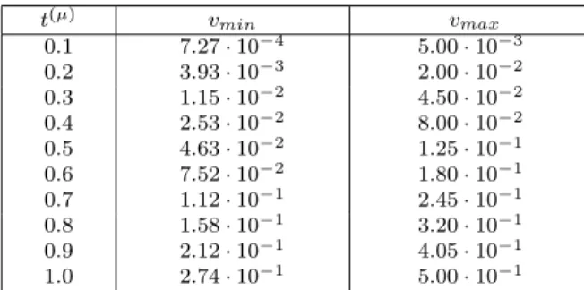
Example 8.2. Consider the porous media equation with absorption
∂tz(t, x, y) =∂xxz(t, x, y) +∂yyz(t, x, y)−[z(t, x, y)]2 (8.3)
with the initial-boundary condition
z(t, x, y) = 1 2t
2 on E
0∪∂0E. (8.4)
The constant functions u0(t, x, y) ≡ 0 and v0(t, x, y) ≡ 12 are, respectively,
a lower and an upper solution of problem (8.3), (8.4). It follows from Theorem 4.1 in [5] (see also Theorem 2.1 in [4]) that this problem has the unique solution
u ∈ C1,2(Ω,R) and u(t, x, y) ∈ 0,1 2
for (t, x, y) ∈ Ω. Note that we can put for instance σ0(t, r) = r2,t ∈[0,1],r∈R+, in Theorem 3.1 (see also Remark 3.2) and
obtain|u(t, x, y)| ≤(2−t)−1 ≤1for(t, x, y)∈Ω. Puttingϕh=ϕ|Ωh,Gh=Th and
σ = σ0 in Theorem 5.3 we have v(µ,m) ≤ 2−t(µ)− 1
≤ 1 for t(µ), x(m) ∈ Ω
h,
wherev is the solution of the implicit difference scheme (5.1) for (8.3), (8.4). Hence, we can putR= [−1,1]in Assumption F∗[f, u, G
h]. Note that this assumption is not
fulfilled forR=R, becausef(t, x, y, z, p, q) =q11+q22−[z(t, x, y)]2 does not fulfill the generalized Perron condition on C(Ω,R). Puth0 =h1=h2 = 10−1. Note that the Courant-Friedrichs-Levy condition (6.8) for such steps is not satisfied. For each
t(µ)we use the method of an inverse matrix to solve the implicit difference scheme. Let
vmin,vmax be the smallest and largest values, respectively, ofvat timet(µ)(Tab. 2).
Table 2. Values ofvmin,vmax
t(µ) vmin vmax
0.1 7.27·10−4 5.00·10−3
0.2 3.93·10−3 2.00·10−2
0.3 1.15
·10−2 4.50·10−2 0.4 2.53
·10−2 8.00·10−2 0.5 4.63·10−2 1.25·10−1
0.6 7.52·10−2 1.80·10−1
0.7 1.12
·10−1 2.45·10−1 0.8 1.58
·10−1 3.20·10−1 0.9 2.12·10−1 4.05·10−1
1.0 2.74·10−1 5.00·10−1
Example 8.3. Consider the strongly nonlinear with a quasi-linear term differential integral equation with deviated variables
∂tz(t, x, y) = arctan [∂xxz(t, x, y) +∂xyz(t, x, y) +∂yyz(t, x, y)] +
+ [2 + cosz(t, x, y)] [∂xxz(t, x, y) +∂xyz(t, x, y) +
+∂yyz(t, x, y)] + [sinz(t, x, y)]∂xz(t, x, y) +
+1 8
t
Z
0 1 Z
−1 1 Z
−1
z(s, a, b)dbdads+ [z(0.5t,0,0)]2+g(t, x, y)
with the initial-boundary condition
z(t, x, y) = 0.01 sintcos (x+y) on E0∪∂0E, (8.6)
where
g(t, x, y) = arctan [0.03 sintcos (x+y)] +
+ 0.01 [cost+ 6 sint+ 3 sintcos (0.01 sintcos (x+y))] cos (x+y) + + 0.01 sintsin (0.01 sintcos (x+y)) sin (x+y) + 0.005 sin21 (cost−1)− −0.0001 sin20.5t.
The function u(t, x, y) = 0.01 sintcos (x+y) is an analytic solution of prob-lem (8.5), (8.6). Obviously, |u(t, x, y)| ≤ 0.01 for (t, x, y) ∈ Ω. Note that we can put for instance σ0(t, r) = 3 r+14
2
, t ∈ [0,1], r ∈ R+, in Theorem 3.1 (see also Remark 3.2) and obtain |u(t, x, y)| ≤ 1
4 4 26+ 3t
100 26 −3t
−1
≤ 41 44
for (t, x, y) ∈ Ω. Putting ϕh = ϕ|Ωh, Gh = Th and σ = σ0 in Theorem 5.3 we have v(µ,m) ≤ 1
4 4 26+ 3t
(µ) 100 26 −3t
(µ)−1 ≤ 41
44 for t
(µ), x(m) ∈ Ωh, where v is the solution of the implicit difference functional scheme (5.1)
for (8.5), (8.6). Hence, we can put R = −41 44,
41 44
in Assumption F∗[f, u, G
h].
Note that this assumption is not fulfilled for R = R, because f(t, x, y, z, p, q) = arctan q11+12q12+12q21+q22
+ [2 + cosz(t, x, y)] q11+12q12+12q21+q22
+ [sinz(t, x, y)]p1+ 18R0tR−11R−11z(s, a, b)dbdads+ [z(0.5t,0,0)]2+g(t, x, y) does not
fulfill the generalized Perron condition on C(Ω,R). Put h0 =h1 =h2 = 10−1. For
eacht(µ) we use one hundred iterations of the Newton method to solve the implicit
difference functional scheme. Let vmin, vmax be the smallest and largest values,
re-spectively, of v at time t(µ) (Tab. 3). Moreover, let ε
max, εmean be the largest and
mean values, respectively, of the errors|U−v|of the difference method (5.1) at time
t(µ) (Tab. 4).
Table 3. Values ofvmin,vmax
t(µ) vmin vmax
0.1 −4.15·10−4 9.98·10−4
0.2 −8.26·10−4 1.98·10−3
0.3 −1.22·10−3 2.95·10−3
0.4 −1.62·10−3 3.89·10−3
0.5 −1.99·10−3 4.79·10−3
0.6 −2.34·10−3 5.64·10−3
0.7 −2.68·10−3 6.44·10−3
0.8 −2.98·10−3 7.17·10−3
0.9 −3.25·10−3 7.83·10−3
1.0 −3.50·10−3 8.41·10−3
Table 4. Errors of the difference method
t(µ) εmax εmean
0.1 4.82·10−4 2.04·10−4
0.2 6.55·10−4 2.69·10−4
0.3 7.04·10−4 2.86·10−4
0.4 7.05·10−4 2.85·10−4
0.5 6.84·10−4 2.75·10−4
0.6 6.50·10−4 2.62·10−4
0.7 6.08·10−4 2.45·10−4
0.8 5.60·10−4 2.25·10−4
0.9 5.06·10−4 2.03·10−4
1.0 4.46·10−4 1.79·10−4
Note that the Courant-Friedrichs-Levy condition (6.8) for such steps is not satisfied and the explicit method given in [14] is not convergent. In fact, the errorsεmax,εmean
of that method exceeded1011and1010, respectively.
Acknowledgements
The results of the paper were presented on the 11th Conference Mathematics in Natural and Technical Sciences, September 8–12, 2010 in Krynica, Poland. The author thanks the Organizers for this possibility.
The research of the author was partially supported by the Polish Ministry of Science and Higher Education.
REFERENCES
[1] U.G. Abdulla,On the Dirichlet problem for reaction-diffusion equations in non-smooth domains, Nonlinear Anal.47(2001), 765–776.
[2] P. Besala, G. Paszek,Differential-functional inequalities of parabolic type in unbounded regions, Ann. Polon. Math.38(1980), 217–228.
[3] S. Brzychczy, Existence and uniqueness of solutions of infinite systems of semilin-ear parabolic differential-functional equations in arbitrary domains in ordered Banach spaces, Math. Comput. Modelling36(2002), 1183–1192.
[4] S. Brzychczy, Monotone iterative methods for infinite systems of reaction-diffusion--convection equations with functional dependence, Opuscula Math.25(2005), 29–99.
[5] S. Brzychczy,Infinite Systems of Parabolic Differential-Functional Equations, AGH Uni-versity of Science and Technology Press, Cracow, 2006.
[6] B.H. Gilding, R. Kersner,Memorandum No. 1585, Faculty of Mathematical Sciences, University of Twente, 2001.
[7] J. Hale, L. Verdyun,Introduction to Functional Differential Equations, Springer, 1993.
[8] H.N.A. Ismail, A.A.A. Rabboh, A restrictive Padé approximation for the solution of the generalized Fisher and Burger-Fisher equations, Appl. Math. Comput.154(2004), 203–210.
[9] Z. Kamont, H. Leszczyński, Stability of difference equations generated by parabolic differential-functional problems, Rend. Mat. Appl. (7)16(1996), 265–287.
[10] Z. Kamont, Hyperbolic Functional Differential Inequalities and Applications, Kluwer Acad. Publ., Dordrecht, Boston, London, 1999.
[11] Z. Kamont, Numerical approximations of difference functional equations and applica-tions, Opuscula Math.25(2005), 109–130.
[12] Z. Kamont, K. Kropielnicka,Implicit difference functional inequalities and applications, J. Math. Inequal.2(2008), 407–427.
[13] K. Kropielnicka,Implicit difference methods for quasi-linear parabolic functional differ-ential problems of the Dirichlet type, Appl. Math.35(2008), 155–175.
[15] M. Malec, Sur une famille biparamétrique de schémas des différences finies pour un système d’équations paraboliques aux dérivées mixtes et avec des conditions aux limites du type de Neumann, Ann. Polon. Math.32(1976), 33–42.
[16] M. Malec, Sur une méthode des differences finies pour une équation non linéaire dif-férentielle fonctionnelle aux dérivées mixtes, Ann. Polon. Math.36(1979), 1–10.
[17] M. Malec, Cz. Mączka, W. Voigt,Weak difference-functional inequalities and their appli-cation to the difference analogue of non-linear parabolic differential-functional equations, Numer. Math.11(1983), 69–79.
[18] M. Malec, M. Rosati,A convergent scheme for non-linear systems of differential func-tional equations of parabolic type, Rend. Mat. Appl. (7)3(1983), 211–227.
[19] M. Malec, L. Sapa,A finite difference method for nonlinear parabolic-elliptic systems of second order partial differential equations, Opuscula Math.27(2007), 259–289.
[20] J.D. Murray,Mathematical Biology, Springer, Berlin, 1993.
[21] C.V. Pao,Nonlinear Parabolic and Elliptic Equations, Plenum Press, New York-London, 1992.
[22] C.V. Pao,Finite difference reaction-diffusion systems with coupled boundary conditions and time delays, J. Math. Anal. Appl.272(2002), 407–434.
[23] R. Redheffer, W. Walter, Comparison theorems for parabolic functional inequalities, Pacific J. Math.85(1979), 447–470.
[24] L. Sapa,Implicit difference methods for differential functional parabolic equations with Dirichlet’s condition, to appear.
[25] L. Sapa,A finite difference method for quasi-linear and nonlinear differential functional parabolic equations with Dirichlet’s condition, Ann. Polon. Math.93(2008), 113–133.
[26] J. Szarski, Differential Inequalities, Monograph, PWN - Polish Scientific Publishers, Warsow, 1965.
[27] J. Szarski, Strong maximum principle for non-linear parabolic differential-functional inequalities in arbitrary domains, Ann. Polon. Math.31(1975), 197–203.
[28] W. Walter,Differential and Integral Inequalities, Monograph, Springer-Verlag, Berlin, Heidelberg, New York, 1970.
[29] J. Wu,Theory and Applications of Partial Functional Differential Equations, Springer, 1996.
Lucjan Sapa
AGH University of Science and Technology Faculty of Applied Mathematics
al. Mickiewicza 30, 30-059 Krakow, Poland