Equações diferenciais fracionárias: um novo estudo de soluções locais e globais em...

Fractional differential equations:

a novel study of local and global solutions

in Banach spaces

Equações diferenciais fracionárias:

um novo estudo de soluções locais e globais

em espaços de Banach

SERVIÇO DE PÓS-GRADUAÇÃO DO ICMC-USP

Data de Depósito:

Assinatura:

Fractional differential equations:

a novel study of local and global solutions

in Banach spaces

Paulo Mendes de Carvalho Neto

Advisor: _{Prof. Dr. Alexandre Nolasco de Carvalho} Co-Advisor: Prof. Dr. Pedro Marín-Rubio

Doctoral dissertation submitted to the Instituto de Ciências Matemáticas e de Computação- ICMC-USP, in partial fulfillment of the requirements for the degree of the Doctorate Program in Mathematics. REVISED VERSION_.

SERVIÇO DE PÓS-GRADUAÇÃO DO ICMC-USP

Data de Depósito:

Assinatura:

Equações diferenciais fracionárias:

um novo estudo de soluções locais e globais

em espaços de Banach

Paulo Mendes de Carvalho Neto

Orientador: _{Prof. Dr. Alexandre Nolasco de Carvalho} Co-Orientador: _{Prof. Dr. Pedro Marín-Rubio}

Tese apresentada aoInstituto de Ciências Matemáticas e de Computação - ICMC-USP, como parte dos requisitos para obtenção do título de Doutor em Ciências.VERSÃO REVISADA_.

USP – São Carlos

A

A

A

A

A

A

A

A

A

A

A

cknowledgement

“Mathematics, rightly viewed, possesses not only truth, but supreme beauty

− a beauty cold and austere, like that of sculpture, without appeal to any part of our weaker nature, without the gorgeous trappings of painting or music, yet sublimely pure, and capable of a stern perfection such as only the greatest art can show. The true spirit of delight, the exaltation, the sense of being more than Man, which is the touchstone of the highest excellence, is to be found in mathematics as surely as poetry.”

Bertrand Russell (1919)

Mathematics can be seen as a different way of understand the life itself. The patterns are hidden in plain sight, we just have to know where to search for them. Things most people see as chaos, or as nonsense, actually follow subtle laws of behavior, a mathematical behavior. Galaxies, ocean, plants, seashells, even things that we are used to treat as common stuff, mobiles, television, computers. The truth of mathematics never lies, but only some of us can see how the pieces fit together to somehow organize this chaotic information and “decode it”, understand and in some way create a new knowledge.

The years studying mathematics during the Master Degree and the PhD still remains one of the happiest times in my life. Also I’m very grateful to all the mathematicians I met during this chapter of my formation, their contagious enthusiasm lead me to continue inspired during all this time. I came to São Carlos many years ago without a clear

First of all, I would like to thank both of my advisors and an important friend and researcher, for the opportunity to study and learn with them. They are models as teachers and mathematicians to all the researchers that are beginning, as myself.

– In Brazil,Prof. Dr. Alexandre Nolasco de Carvalho, was my mentor in many ways, teaching in courses, in life and on the research itself. He is responsible for most of all my math training, and for that, I have an immense gratitude. I will never forget the puzzled look he gave me when I introduced myself and, in the same breath, asked him to be my thesis advisor. Also, I can’t forget the day that he introduce me to my thesis final objective. At the beginning, the fractional differential equations seemed so odd, but with time and dedication, once again I noticed that Alexandre was right, when he told me at that first day what a wonderful puzzle-world I was being introduced.

–And during my research time in Spain,Prof. Dr. Pedro Marín Rubio, was a father and a friend in the life on a new country, but with him besides of learning mathematics, he taught me how to understand and observe the details on the math-world. I clearly remember the first day in July of 2011 when we first met and began to study together. His support, insight and enthusiasm have fueled this process from beginning to end. In addition, he showed great patience and understanding in dealing with a foreign student that barely spoke his language.

– Finally during my two last years of research, Prof. Dr. Bruno Luis de Andrade Santos was an important mathematician and friend that inspired and helped me during all the studies done in this thesis. I really want to thank him for all the afternoons and nights that we spent discussing mathematical problems. I hope he continues to collaborate with me during the rest of my career.

Their contributions to one of the most significant chapters of my life will never be forgotten.

It’s important to say that all the personal from both departments ICMC-USP in São Carlos/Brazil and EDAN-US in Sevilla/Spain were extremely helpful and ready to help me with any bureaucracy or problems of institutional nature. In particular, I thank for the seminars, for the meetings and all the sharing between the people involved with the group of differential equations from both places.

Next I want to thank all my friends. I wouldn’t have been able to write this thesis without their support, but I have so many names to remember that it seems an almost impossible task. Even if I tried, I’m afraid this acknowledges would grow longer than the body of my thesis... So, as I have just this small piece of paper to write everything I want,

it looks better to be subtle. In few words, I can say that apart of being distant from some of them during different periods, the way that lead me to this final text was certainly guided in parts for their friendship, companionship and for the importance that each one of us has in the life of the other. Be known that once we’ve met, we became hard-wired with the impulses to share our ideas, to be connected in many ways, to understand each other... this is the family I was able to choose each of its members, becoming my brothers and sisters, the ones I choose to share happiness, sorrows, victories and defeats, hands to lift me up and shoulders to lean on. Thus, the only words I can image to write here are:

Thanks for everything, for each second, for each word... I’m very happy to have the opportunity to call them friends.

Now I want to thank my family for everything they’ve done for me, their support and comprehension during my studies. I owe my family an immeasurable debt of gratitude for their unwavering support of my ever endeavor, despite my repeated selection of distant universities. My first and greatest teachers were my parents, Armando e Odete. I can’t tell just in words how much I’m happy to have them as my first teachers. My Father was a beacon in my life, teaching me and understanding my choice (to him so odd) of the academic and research work. For that I consider myself a lucky guy. And my Mom, that was always there to help me and to stand by me whenever was needed (even when she couldn’t understand the real problem). Her ability to find kind words at the most difficult times meant more that mere words can convey. She isn’t here today to see the result of all the effort, but I know that if she were, she would be very proud. There wasn’t a single day, that I haven’t thought in you.

And in special, I want to say some words to someone that just started to have a very important role in my life. Sometimes we just don’t get what wonderful gifts life gave us, but when we notice and understand that even in a gray and bitter time, just a word or a look is sufficient to make everything get colored and sweet again, you can consider yourself special. That spark sunk deeply in your eyes guided me for a long time and still guide... So I wish to thank you so much,Mariana, that just the word “thanks” isn’t enough to mean it. I love you so much.

The major part of the studies done during the PhD where in São Carlos/Brazil under the supervision of Prof. Dr. Alexandre, financed in the first months byCNPqand during all the rest of the time byFAPESP. The major part of the Thesis was written on Sevilla/Spain, during the study in the Sandwich-PhD under the supervision of Prof. Dr. Pedro, financed byCAPES.

R

R

R

R

R

R

R

R

R

R

R

esumo

Motivados pelo êxito das aplicações nas equações abstratas em muitas áreas da ciência e da engenharia, e pelas perguntas ainda abertas, neste trabalho estudamos questões relativas aos problemas fracionários abstratos de Cauchy de ordemα_∈(0,1). Buscamos responder algumas perguntas: por exemplo, analisamos a existência de soluções locais fracas do problema e sua possível continuação em um intervalo maximal de existência. O caso da não-linearidade crítica e sua correspondente solução regular fraca também é abordado. Por último, mediante o estabelecimento de alguns resultados gerais de comparação, chegamos a conclusão de que as soluções de uma equação diferencial parcial fracionária, proveniente da teoria de condução de calor, existe globalmente.

R

R

R

R

R

R

R

R

R

R

R

esumen

Motivados por el éxito de las aplicaciones de las ecuaciones abstractas fraccionarias en muchas áreas de la ciencia y la ingeniería, y por las preguntas abiertas en esta teoría, en este trabajo se estudian varias cuestiones relativas a los problemas abstractos de Cauchy fraccionarios de ordenα_∈(0,1). Buscamos responder a algunas preguntas que estaban abiertas: por ejemplo, se analiza la existencia de soluciones locales debiles del problema, y su posible continuación a un intervalo maximal de existencia. En el caso de la no linealidad crítica, también se estudia la existencia de la correspondiente solución regular débil. Por último, mediante el establecimiento de algunos resultados generales de comparación, llegamos a la conclusión del buen planteamiento de una solution global de una ecuación diferencial parcial fraccionaria, procedente de la teoría de la conducción del calor.

A

A

A

A

A

A

A

A

A

A

A

bstract

Motivated by the huge success of the applications of the abstract fractional equations in many areas of science and engineering, and by the unsolved question in this theory, in this work we study several matters related to abstract fractional Cauchy problems of order

α_∈(0,1). We search to answer some questions that were open: for instance, we analyze the existence of local mild solutions for the problem, and its possible continuation to a maximal interval of existence. The case of critical nonlinearities and corresponding regular mild solutions is also studied. Finally, by establishing some general comparison results, we apply them to conclude the global well-posedness of a fractional partial differential equation coming from heat conduction theory.

Contents

Page

Introduction 1

1 Preliminary Knowledges 11

1.1 General results _{· · · ·} 12

1.2 Linear operators, semigroups and evolution equations _{· · · ·} 14

1.3 Fractional powers · · · 18

2 Fractional Calculus 21 2.1 Tools and special functions · · · 21

2.2 Fractional integration and derivation · · · 37

2.3 Fractional differential equations - bounded operators · · · 44

2.4 The Mittag-Leffler operators · · · 47

3 Abstract Fractional Equations 59 3.1 Existence, uniqueness and the fractional limit · · · 61

3.2 Comparison and global existence of solutions _{· · · ·} 80

3.3 The critical case _{· · · ·} 91

4 Some Comments on Open Problems and Remaining Questions 109

Bibliography 115

IIIIIIIIII

I

ntroduction

At a first glance, when we begin to study the fractional derivative and fractional integral, we can be a little unwilling, thinking how odd is the definition and how difficult it can be to be manipulated. But for instance, when we return to our primary school knowledge, and remember that we used to learn that exponents provide a short notation for what is essentially a repeated multiplication of a numerical value, the physical definition can clearly become confused when considering exponents of non integer value. Almost anyone can relate that x4 _{= x}

· x_· x _·x, but how can an ordinary person describe the physical meaning of x5,4_{, or moreover the transcendental exponent in x}π_{. One cannot conceive} what it might be like to multiply a number or quantity by itself5,4times, orπtimes, and yet these expressions have a definite value, verifiable by infinite series expansion. Now in the same way, consider the integral and the derivative. Although they are indeed concepts of a higher complexity by nature, it is still fairly easy to physically represent their meaning and their relation with the positive integer numbers. Our question arrives when we try to think as done before and change the integer number of derivation or integration exponent to a fractional number. In this direction, we will study other operators, sometimes called fractional differentiation or integration operators. In this text, one notices that this definition follows naturally.

B

ACKGROUNDS

The fractional calculus can be considered in many ways, a novel topic, once it is only during the last thirty years that it has been the subject of specialized conferences and treatises. Everything has begun with the important applications discovered in numerous diverse and widespread fields in science, engineering and finance. More specifically, we can easily find a direct application of fractional calculus in the study of Fluids Flow,

Porous Structures, Control Theory of Dynamical Systems, Rheology Theory, Viscoelasticity, Chemical Physics, Optics, Signal Processing and in many other problems, see[13, 58, 59, 60, 61, 75]among others. One can also read on many specialized texts, that the fractional derivatives and integrals are very suitable for modeling the memory properties of various materials and processes that are governed by anomalous diffusion(term used to describe a diffusion process with a non-linear relationship to time).

It is important to understand that the concept of fractional calculus is not a new one, even we already said that it is a novel topic. The history is believed to have emerged from a question raised in the year 1695 by Marquis de L’Hôpital to Gottfried Wilhelm Leibniz. In his letter, L’Hôpital asked about a particular notation Leibniz had used on his publications for the derivative. He used to write

dn d xnf(x)

to symbolize the n-th derivative of a function f, to n_∈N∗_{:={1,2, . . .}. L’Hôpital posed his}

question, arguing about the possibility of takingn=1/2. In his reply, dated 30 September of 1965, Leibniz wrote back saying

“... This is an apparent paradox from which, one day, useful consequences will be draw. ...”

Following this line, in 1730, Euler mentioned interpolating between integral orders of a derivative, in 1812 Laplace defined a kind of fractional derivative by means of an integral, and in 1819 there appeared the first discussion of fractional derivative on a calculus text written by S. F. Lacroix. In his 700-page book entitled“Traité du Calcul Différentiel et du Calcul Intégral”, he answered the question, giving as result, that

d1/2

d x1/2x =

2px p_π .

With this answer, formally the fractional calculus was born[42, 47].

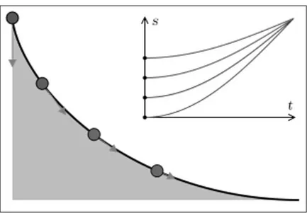
Even Fourier mention the fractional derivatives but did not gave applications or at least examples. So been the first to make applications, N. H. Abel in 1823[1]studied the fractional calculus in the solution of an integral equation which arises in the formulation of the tautochrone problem: it consist in finding the shape of a frictionless wire lying in a vertical plane such that the time of slide of a bead placed on the wire slides to the lowest point of the wire in the same time regardless of where the bead is placed. The brachistochrone problem deals with the shortest time of slide.

Backgrounds 3

Figure 1:

Tautochrone Curve

an infinite series and as we know, the notion of convergence ever would interfere in the definition itself, what was his first obstacle. It was Liouville’s second definition that solved the last problem. The notion adopted for the fractional differential of an integrable function f : [t0,t1]⊂R→Rwas

t0D α

t f(t) =

1

Γ(m−α) _dm

d tm

Zt t0

(t−s)m−α−1_{f(s)ds, t}

∈[t0,t1]

whereα >0andmis the first integer greater or equal thanα.

As the last advance, in order to present a notion more compatible with the usual theory of differential equations, comes the notion introduced by M. Caputo in 1967 in his celebrated paper [18]. In contrast to the Riemann-Liouville fractional derivative, when solving differential equations using Caputo’s definition, it is not necessary to deal with the singularity on t = 0 and define the fractional order initial conditions, which eventually could be unpleasant to the physics theory. Caputo’s definition is illustrated for regular functions f : [t0,t1]⊂R→Ras follows

ct0D α

t f(t) =t0D α

t



f(t) −

m−1

X

k=0

dkf(t)

d tk

!

t=t0

(t−t0)k

k! 

, t∈[t0,t1]

where we also have thatα >0and mis the first integer greater or equal thanα.

that solutions in closed form have been found only for such equations with constant coefficients and for a rather small class of equations with particular variable coefficients. In general, numerical solution techniques are required to obtain more precise answers. We cannot forget to relate the fundamental and basic role of Mittag-Leffler type functions to “represent” the solutions in this theory. The most simple function of Mittag-Leffler type, Eα(z)for example, depends on two variables: the complex argument z and the real parameterα. Experience in the computation of special functions of mathematical physics teach us that these functions behave in huge different way in distinct parts of the complex plane which make us think in how strongly this information could affect the abstract computations and proofs.

A practical example to the study of the fractional differential equations comes when one tries to understand aRheological Constitutive Equationson the basis of well known mechanics models, i.e., the study of the flow of matter, primarily in the liquid state, but also as “soft solids” or solids under conditions in which they respond with plastic flow rather than deforming elastically in response to an applied force. With some physics manipulations and assumptions, we deduce the following equations:

σL(t) +C1c D

α−β

t σL(t) =C2c Dαtε(t),

σR(t) =C3c D

γ

tε(t)

where γ _∈(0,1), 0 < β < α < 1, C_i for i _∈{1,2,3} are positive constants, σ_L(t) is the stresses in the left, σR(t) the stresses in the right and ε(t) is the strain. This model is

the so-calledZener Modelor the standard solid model. This is a method of modeling the behavior of a viscoelastic material using a linear combination of springs and dashpots to represent elastic and viscous components, respectively(More details in[60]).

T

HESIS

O

BJECTIVES AND

O

UTLINES

The study of the fractional differential equations found place in several different topics, already discussed and solved for the usual differential equations. Among all these topics, one that stands out is the study of the abstract Cauchy problems with the Caputo fractional derivative, when we consider the fractional exponentα_∈(0,1).

Thesis Objectives and Outlines 5

instance[11, 26, 30, 36, 41, 53, 55, 66, 67]. Our objective is to study some new properties and relations between the ordinary theory and the fractional theory.

So motivated by this we consider the abstract fractional Cauchy problem

c Dα_tu(t) = −Au(t) +f(t,u(t)), t>0 u(0) =u0∈X,

(1)

where X is a Banach space, α_∈(0,1), A: D(A)_⊂ X _→ X is a positive sectorial operator,

c Dα_t is the Caputo fractional derivative and f : [0,_∞)_×X _→X is a suitable function. In order to start our discussion, let us recall some preliminaries. We understand as the Caputo fractional derivative(see Section 2.2 to a better definition)the operator

c Dα_tu(t) =Dα_t

u(t) −u(0),

where Dα_t is the Riemann-Liouville fractional derivative, that is given by

Dα_tu(t) =D_t 1

Γ(α)

Zt 0

(t−s)α−1u(s)ds.

Consider also {Eα(−tαA) : t ≥ 0} and {Eα,α(−tαA) : t ≥ 0} the Mittag-Leffler families associated to−A (see Section 2.4 for details). We adopt the following concepts for solutions to problem (1).

i) A functionu: [0,_∞)_→X is said to be a global mild solution to problem (1) in[0,_∞) if uis continuous and

u(t) =Eα(−tαA)u0+

Zt 0

(t−s)α−1Eα,α(−(t−s)αA)f(s,u(s))ds, t≥0. (2)

ii) Letτ >0. A functionu: [0,τ]_→X is said to be a local mild solution to problem (1) in[0,τ]ifu_∈C([0,τ];X)and

u(t) =Eα(−tαA)u0+

Zt 0

(t−s)α−1Eα,α(−(t−s)αA)f(s,u(s))ds, t∈[0,τ].

Our main purpose in this work is to ensure sufficient conditions for existence and uniqueness of solution to (1) and to establish some regularity and comparison results for this solution on Banach spaces.

is fundamental to the basic estimates and constructions that will be recurrently used during all this text.

InChapter 2, the emphases are the fractional calculus and the Mittag-Leffler functions, that plays an important role in this theory. Among other things, we study some properties of the gamma function, the beta function and other special functions. In particular, we study the behavior of the families {Eα(−tαA) : t ≥ 0} and {Eα,α(−tαA) : t ≥ 0} on the fractional power spaces associated to the positive sectorial operator A and we establish expressions for these families, similar to the second fundamental limit for semigroups.

InChapter 3, we finally consider the new results. We devote theSection 3.1to study existence, uniqueness and continuation results to (1) when the nonlinear term is a locally Lipschitz continuous function f : [0,_∞)_×X _→X. In this direction we want to obtain an argument to guarantee the existence of global solution or the “Blow-Up” of maximal local mild solutions. The first important theorem of this section is the following:

Theorem Let f : [0,_∞)_×X _→ X be a continuous function, locally Lipschitz in the second variable, uniformly with respect to the first variable, and bounded (i.e. it maps bounded sets onto bounded sets). Then the problem(1)has a global mild solution in[0,_∞)or there exists

ω _∈(0,_∞) such that u : [0,ω)_→ X is a maximal local mild solution, and in such a case,

lim sup_t→ω−ku(t)k=∞.

Finally, we consider forγ_∈(0,1]the problem

c Dγtu(t) = −Au(t) +f(t,u(t)), t≥0

u(0) =u0∈X,

(Pγ)

where c Dγt is the Caputo fractional derivative, A: D(A) ⊂ X → X is a positive sectorial

operator and the function f : [0,_∞)_×X _→ X is globally Lipschitz and prove the latest important theorem in this section.

Theorem Consider the problem (Pγ), forγ∈(0,1]and suppose that uγ(t)is the maximum

local mild solution of (Pγ)defined over[0,ωγ). Then there exists t∗>0 such that

[0,t∗]_⊂ \ γ∈[1/2,1]

[0,ωγ)

and for each fixed t∈[0,t∗]

lim γ→₁−k

uγ(t) −u1(t)k=0.

Thesis Objectives and Outlines 7

positivity of the families{Eα(−tαA) : t ≥ 0} and {Eα,α(−tαA) : t ≥ 0} with the positivity of the functionλ_7→(λα+A)−1_{. With respect to the semilinear problem (1), we establish}

results on the positivity of the solutions to conclude the following comparison result.

Theorem Let (X,_≤X) be an ordered Banach space and suppose that the families

{Eα(−tαA) :t≥0}and{Eα,α(−tαA) :t≥0}are increasing.

i) Let u0,u1∈X , and assume that there exist t0, t1 ∈[0,∞)such that{uf(t,ui)}i=0,1 are

local mild solutions in[0,ti],i∈{0,1}, to

c Dα_tu(t) = −Au(t) + f(t,u(t)), t>0,

u(0) =ui∈X.

Then, if t∗ =min{t0,t1}, f(t,·) is increasing a.e. t ∈[0,t∗],and u1 ≤X u0, it holds

that uf(t,u1)≤X uf(t,u0)for all t ∈[0,t∗].

ii) Consider functions f0 and f1,and u0 ∈X , and assume that there exist t0, t1 ∈[0,∞)

such that{ufi(t,u0)}i=0,1are local mild solutions in[0,ti],i∈{0,1}, to

c Dα_tu(t) = −Au(t) +fi(t,u(t)), t>0,

u(0) =u0∈X.

Then, if t∗ =min{t0,t1}and f0(t,x)≤X f1(t,x)a.e. t ∈[0,t∗] and for all x ∈X , it

holds that uf0(t,u0)≤X uf1(t,u0)for all t ∈[0,t

∗_].

iii) Consider functions f0and f1,and u0,u1∈X , and assume that there exist t0,t1∈[0,∞)

such that{ufi(t,ui)}i=0,1 are local mild solutions in[0,ti],i∈{0,1}, to

c Dα_tu(t) = −Au(t) +fi(t,u(t)), t>0,

u(0) =ui ∈X.

Then, if t∗ =min{t0,t1}, and x ≤X y imply f0(t,x)≤X f1(t,y) a.e. t ∈[0,t∗], and

u_0≤X u₁, it holds that u_f0(t,u₀)_≤X u_f1(t,u₁)for all t _∈[0,t∗].

Finally, as an application of this last result we ensure existence of global mild solution for a fractional partial differential equation coming from heat conduction theory.

In order to state a brief resume to this section, let us introduce some notation. For

β _≥0, let Xβ =_D(Aβ) be the fractional power spaces associated to the positive sectorial operatorA. In this section we use the following concepts.

Definition A continuous function u: [0,τ]_→X1 is called a localε-regular mild solution to (1) ifu∈C((0,τ];X1+ε)and verifies (2) in[0,τ].

Definition Forε >0we say that a map g is anε-regular map relative to the pair (X1,X0) if there exist ρ > 1, γ(ε) with ρε _≤ γ(ε) < 1, and a positive constant c, such that

g:X1+ε_→Xγ(ε)and

kg(x) −g(y)_kXγ(ε)≤c €

1+_kxkρ−_X1+1ε+kyk

ρ−1 X1+ε

Š

kx−ykX1+ε,

for allx,y ∈X1+ε.

Next theorem is the main result of Section 3.3 (where details of the suitable class of functions_F(ε,ρ,γ(ε),c,ν(_·),ξ)are given).

Theorem Let α _∈ (0,1) and f _{∈ F}(ε,ρ,γ(ε),c,ν(_·),ξ). If v_{0 ∈} X1_{, there exist positive}

numbers r and τ0 such that for any u0 ∈ BX1(v₀,r) there exists a continuous function

u(_·,u0) : [0,τ0] → X1 with u(0,u0) = u0, which is a local ε-regular mild solution to the

problem

c Dα_tu= −Au+f(t,u(t)), t>0 u(0) =u0.

This solution satisfies

u∈C((0,τ₀];X1+θ), 0≤θ < γ(ε),

lim

t→₀+

tαθku(t,u0)kX1+θ =0, 0< θ < γ(ε).

Moreover, for eachθ₀ < γ(ε)there exists a constant C =C(BX1(v₀,r))>0 such that for any

u₀,w_0∈B_X1(v₀,r),

tαθku(t,u0) −u(t,w0)kX1+θ ≤Cku₀−w₀k_X1 ∀t∈[0,τ₀], 0≤θ ≤θ₀.

In particular we obtain an existence theorem in X1 _{without the nonlinearity being}

defined onX1. Finally, as an application of this last result we ensure existence of a local mild solution for the fractional partial differential equation coming from heat conduction theory.

Thesis Objectives and Outlines 9

1

1

1

1

1

1

1

1

1

1

1

Preliminary Knowledges

T

his first chapter contain some concepts and knowledge used throughout the course of the thesis and has the objective to be a library of basic results. In short, we shall discuss some basic and classical results of operators in Banach spaces and their implications. We begin fixing the notation and establishing important definitions. Then we study linear operators and the existence ofC0-semigroups associated to sectorial operators.

Finally, we study the fractional power of sectorial operators, in order to obtain estimations and interesting properties. We assume that the reader has prior knowledge of the contents in this chapter, which will not be proved.

Unless otherwise noted, throughout this manuscript we consider that N_, Z_, R _and C

are notations to set of the Natural, Integer, Real and Complex numbers. Also, we always consider (X,k · kX) and (Y,k · kY) as notation to Banach spaces (i.e. a complete normed

vector space)over C_{and L}(X,Y)as the space of all linear and continuous maps from X

toY, with the norm

kBkL(X,Y):= sup

kxkX≤1

kB xkY.

We shall use_L(X)to symbolize the space_L(X,X). Furthermore, letB:D_⊂X _→Y be a linear map.

i) The mapBis said to be aclosed mapif the graph set ofB

G(B) ={(x,B x)_∈X ×Y :x ∈D}

is a closed subset of X_×Y.

ii) The mapBis said to be adensely defined map, if the domain ofBis a dense subset ofX.

iii) When Y =X, we will say thatB is alinear operator.

Remark 1.1 To simplify this reading, we emphasize:

i) for any linear mapB:D⊂X _→Y, we will useD(B)(=D)to denote its domain and

R(B)to denote its range;

ii) and whenever there is no possibility of confusion, we shall discard the notation of the norm with a subscript as defined above, writing instead just _{k · k}.

Theorem 1.2(Closed graph theorem) Let B:X →Y be a linear map. If B is a closed map, then B is continuous.

§ 1.1

G

ENERAL RESULTS

We begin studying the overall results of Functional Analysis in Banach spaces. More explicit considerations and proofs of the following results can be found in[15, 28, 43, 63]. As usual in Complex Analysis, we introduce some tools to deal with vector functions

f :_D(f)_⊂C_{→X and explain how the classical results behave in this new frame.} Remark 1.3 Let[a,b]_⊂R_{. If}γ: [a,b]_→C_{is a continuous function, then:}

i) It is called asimple path(or justpath)in the Complex plane.

ii) If it is a differentiable function, we call it asmooth path.

iii) Ifγ(a) =γ(b), we call it aclosed path.

iv) And if there exists a constant M ≥0such that for any partition

P:=a=t0<t1<. . .< tnP =b

of[a,b]the sum

v(γ,P) :=

nP

X

i=1

|γ(ti) −γ(ti−1)|≤ M,

1.1. General results 13

Theorem 1.4(Riemann-Stieltjes integral) Consider a pathγ: [a,b]_⊂R_→C_{with bounded} variation and a vectorial function f : [a,b]_⊂R_{→X . Then there exists a vector I ∈X with} the following property: Givenε >0, there existδ >0 such that, if

P:=a=t₀< t₁<. . .< t_nP =b

is a partition of[a,b]with kPk:=max{ti−ti−1 :1≤i≤nP}< δ, then

I−

np

X

i=1

f(τi)[γ(ti) −γ(ti−1)]

< ε,

for any choose ofτ_{i ∈}[ti−1,ti], 1≤i ≤nP. We denote this vector for

Zb a

f dγand call it the

Riemann-Stieltjes integralof f over the pathγ.

Now we consider the contour integral when the domain of a vectorial function is the complex plane.

Definition 1.5(Contour integral) Letγ: [a,b]_⊂R_→C_{be a path with bounded variation}

and f :{γ}_⊂C_{→ X a continuous vectorial function. Thecountour integral of f overγ}

is defined as _Z

b

a

(f _◦γ)dγ

where the above integral is considered on Riemann-Stieltjes sense. We shall denote it by

Z

γ

f(z)dz.

Proposition 1.6 Letγ: [a,b]_⊂R_→C_{be a smooth path and f :{γ}⊂}C_{→X a continuous} vectorial function. Then

Z

γ

f(z)dz=

Zb a

f(γ(t))γ′(t)d t.

Definition 1.7 (Holomorphic functions) Let Ω _⊂ C _{be an open set and f} : Ω _→ X a vectorial function. If for allλ_∈Ω there exist f′(λ)_∈X such that

lim

z→_λ

f(z) −f(λ)

z−λ −f

′_(λ)=0,

we say that f isholomorphicand we call f′:Ω_→X thederivativeof f.

Definition 1.8 Let Ω _⊂ C_{. We say thatΩ is a Cauchy domain if it has a finite number}

paths, positively oriented (+∂ Ω).

Theorem 1.9 (Cauchy theorem) Let Ω _⊂ C _{be a Cauchy domain and f : Ω → X be a} continuous function that is holomorphic inΩ. Then

Z

+∂ Ω

f(z)dz=0.

Moreover, for anyλ_∈Ω,

f(λ) = 1

2πi

Z

+∂ Ω

f(z)

z−λdz.

Theorem 1.10(Cauchy general theorem) IfΩ_⊂C_{is a Cauchy domain and f} :Ω_→X is a continuous function that is holomorphic inΩ, then f is infinitely differentiable inΩ and for anyλ_∈Ω,

f(n)(λ) = n!

2πi

Z

+∂ Ω

f(z) (z−λ)n+1 dz

for any n_≥0.

§ 1.2

L

INEAR OPERATORS

,

SEMIGROUPS AND EVOLUTION EQUATIONS

In this section we discuss spectral properties of linear operators and semigroups. More details can be found in[15, 33, 63, 76].

Definition 1.11 LetB:_D(B)_⊂X _→X be a linear operator. The set

ρ(B) ={λ_∈C_{: (λI−B)}−1_{:R(λI−B)⊂X →X is injective, bounded andR(λI−B) =X}}

is calledresolvent setofB. The complementary of this set,σ(B) =C_{\ρ(B), is called the} spectrumof B. Forλ_∈ρ(B)the operator(λI−B)−1 _{is called theresolvent.}

From this point on, to simplify the notation, we will omit the identity operator when writing(λI −B), writing just(λ−B).

Theorem 1.12 (Resolvent equality) Let B :_D(B) _⊂ X _→ X be any linear operator. Then, forλ,µ_∈ρ(B), we obtain

(λ−B)−1− (µ−B)−1= (µ−λ)(µ−B)−1(λ−B)−1.

Remark 1.13 If B :_D(B)_⊂ X _→X is a closed linear operator, then by the Closed Graph theorem, for eachλ_∈ρ(B)the application(λ−B)−1_{is an everywhere defined continuous}

1.2. Linear operators, semigroups and evolution equations 15

Definition 1.14 Astrongly continuous semigroup of linear operatorson X is a family

{T(t) :t_≥0}_{⊂ L}(X)such that:

i) T(0) =IX, where I =IX is the identity operator inX.

ii) For any t,s≥0

T(t)T(s) =T(t+s).

iii) The mapR+_{×X ∋}(t,x)_→T(t)x _∈X is continuous. An immediate conclusion of the above properties is

T(t)T(s) =T(t+s) =T(s)T(t),

that is, the family{T(t) :t _≥0}is commutative in respect to the composition.

Remark 1.15 Note that whenever there is no possibility of confusion, from this point on, we will call the family{T(t) :t≥0}described in the last definition, just byC0-semigroup.

Definition 1.16 Let {T(t) : t ≥ 0} _{⊂ L}(X) be a C0-semigroup on X. Its infinitesimal

generatoris the linear operator B:_D(B)_⊂X _→X, where

D(B) :=

x _∈X : lim

t→₀+

T(t)x−x

t exists

and

B x := lim

t→0+

T(t)x−x

t , for all x ∈ D(B).

Theorem 1.17 Suppose that{T(t) :t_≥0}_{⊂ L}(X)is a C0-semigroup on X . Then:

i) If B : _D(B) _⊂ X _→ X is the infinitesimal generator of {T(t) : t _≥ 0}, then B is a closed and densely defined linear operator. Also, for any x _{∈ D}(B) the application

[0,_∞)_∋t_→T(t)x _∈X is continuously differentiable and d

d tT(t)x =BT(t)x =T(t)B x, t>0.

ii) T_m≥1D(Bm)is dense in X .

iii) There existσ >0 such that ifRe(λ)> σ, thenλ_∈ρ(B)and

(λ−B)−1x =

Z∞

0

Theorem 1.18(Second fundamental limit theorem) Let{T(t) : t ≥0}be a C0-semigroup

on X . If B:_D(B)_⊂X _→X is its infinitesimal generator, then T(t)x= lim

n→+∞ 

I− t

nB

‹−n

x= lim

n→+∞ _n

t

_n

t −B

‹−1

B

n

x.

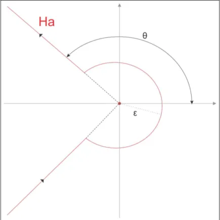
We now describe an important curve in the complex plane, that will be used throughout the text. This path was first used to study the gamma function in the complex plane. Today it is an important path as tool in one of the methods of complex contour integration.

Figure 1.1:

Hankel’s path

Definition 1.19 We say that H a is aHankel’s pathif there existε >0andθ _∈(π/2,π) whereH a=H a1+H a2−H a3 and the paths H ai are given

H a=

      

H a1 :={t eiθ :t∈[ε,∞)}

H a2 :={εei t :t∈[−θ,θ)}

H a3 :={t e−iθ :t∈[ε,∞)}

.

1.2. Linear operators, semigroups and evolution equations 17

above).

Finally, the following constructions provides a brief description of the basic results of the theory of analytic semigroups which forms a functional analytic background for the study done in this manuscript. We start discussing the sectorial operators, using the notation of Henry at[33](for more detailed information see also [39, 40]).

Figure 1.2:

Sector

S

_φ,a

Definition 1.20 Let A : _D(A) _⊂ X _→ X be a closed and densely defined operator. The operator A is said to be a sectorial operator if there exist constants a _∈ R_{, N ≥ 1 and}

φ_∈(0,π/2)such that

Sφ,a:={λ∈C : φ≤|arg(λ−a)|≤π}⊂ρ(A)

(see Figure 1.2 above)and

k(λ−A)−1_kL(X)≤

N

|λ−a|, ∀λ∈Sφ,a\ {a}.

and write justSφ to represent its sector.

Theorem 1.22 If A:_D(A)_⊂X _→X is a sectorial operator, then−A generates an C0-semigroup

{T(t) :t_≥0},

T(t) =

Z

−a+H a

eλt(λ+A)−1dλ

where−a+H a is the shift of any Hankel’s path (as in Definition 1.19) contained inρ(−A). Moreover, there exist C>0 such that

kT(t)_kL(X)≤C e−at, kAT(t)kL(X)≤(C/t)e−at

for all t>0. Finally, for any x ∈X the function[0,_∞)_∋t7→T(t)x ∈X is analytic and d

d tT(t)x = −AT(t)x

for t>0.

§ 1.3

F

RACTIONAL POWERS

The study of fractional powers of operators has a long history, which may go back to Abel’s work on the tautochrone, the Riemann-Liouville integral, and its generalizations by M. Riesz. The problem of finding a suitable representation for a fractional power of an unbounded operator defined on a Banach space X has attracted much attention and in this section, we study this theory whenA:_D(A)_⊂X _→X is a positive sectorial operator. Properties associated with these fractional powers will then be established in a natural manner as a framework to the study that follows.

The fractional powers of sectorial operators play a fundamental role in the theory of existence of solutions to non-linear partial differential equations of parabolic type and to analysis of the asymptotic behavior of solutions to these problems. For more information see[5, 6, 7, 33].

Definition 1.23 LetAbe a positive sectorial operator onX andβ >0. Then we define

A−β = 1

Γ(β)

Z∞

0

sβ−1T(s)ds

where{T(t) :t_≥0}is the C0-semigroup generated by−A.

1.3. Fractional powers 19

Proposition 1.25 Let A be a positive sectorial operator on X . Then for any β _≥ 0 the operator A−β_{∈ L}(X)and it is injective. Moreover, ifβ andδare non negative real numbers, then

A−βA−δ=A−(β+δ).

The above construction guarantees the existence of a bijective operator into its range, for any positive sectorial operator. Now we want to define an operator that play the same role that the fractional positive powers of bounded operators. Supported by Proposition 1.25 we can define the fractional power ofA, for anyβ _≥0, as

Aβ :_D(Aβ)_⊂X _→X, where_D(Aβ) :=_R(A−β)andAβ := (A−β)−1_.

Proposition 1.26 Let A be a positive sectorial operator on X . Then for any α,β _≥ 0 we observe that

i) Ifβ >0, then Aβ is a closed and densely defined operator.

ii) Ifα_≥β, then_D(Aα)_{⊂ D}(Aβ).

iii) AαAβ =AβAα =Aα+β on_D(Aγ), whereγ=max{α,β,α+β}.

iv) AαT(t) = T(t)Aα on _D(Aα), for t > 0, where {T(t) : t _≥ 0} is the C0-semigroup

generated by−A.

Theorem 1.27 Let A be a positive sectorial operator in X andβ _∈(0,1), then

kAβ(λ+A)−1x_kX ≤C|λ|β−1kxkX,

for any x _∈X and anyλin the sector of the operator−A.

Now we start to define important fractional spaces that will be used on the chapters that follows.

Definition 1.28 LetAbe a positive sectorial operator onX. Consider for eachβ_≥0

Xβ =_D(Aβ)

with the graph norm

kx_kXβ =kAβxk_X

These spaces defined above will provide the topology used on Section 2.4 and on Section 3.3, so we just cite a last theorem that collect certain properties, merely reformulating the theorems proved until now.

2

2

2

2

2

2

2

2

2

2

2

Fractional Calculus

O

ne of the essential knowledge for the study that follows, is the notion of fractional calculus. Therefore this chapter is concerned with the study of some concepts and results in Banach spaces to familiarize the reader with this kind of calculations. We start studying the usual notations and the basic definitions. Then we focus on the study of the fractional operators(of integration and differentiation).

It is also important to understand that in this chapter we will study two fractional differential operators(the Riemann-Liouville and the Caputo). However, our objective is to consider the Caputo fractional differentiation operator on the abstract Cauchy problems that we will study on Chapter 3.

§ 2.1

T

OOLS AND SPECIAL FUNCTIONS

In this section, we study some preliminary concepts related to the fractional calculus(for more details, see, for instance,[12, 27, 42]).

To begin this section, we recall the study of the locally Bochner integrable functions and the Lp-spaces (1 _≤ p < _∞) for the Dunford-Schwartz integral with respect to a Banach space [25, Chapter 3]. This theory of integration over vector valued functions was constructed by Bochner in[14]. ConsiderS⊂R_{and the following Banach spaces, in}

the sense of Bochner.

• (Lp_{(S,X),k · k}

Lp_(S,X)), for1≤p<∞, denotes the set of all measurable functions on

S to X such that_ku(t)_kXp is integrable and its norm is given by

ku(t)_kLp_(S,X):= Z

Sk

u(t)_kp_Xd t

1/p

.

• Lp

l oc(S,X), for 1≤ p< ∞, denotes the space of functions that belongs to L

p_(S˜,X)

for all ˜S _⊂⊂S (compactly contained). These functions are called locally integrable functions.

• (Wp,k_{(S,X),k · k}

Wp,k_(S,X)), denotes the space of functions f ∈ Lp(S,X)which have

weak derivative of order less or equal then k, all being on Lp_{(S,X), with norm}

ku(t)_kWp,k_(S,X):= k

X

n=0

Z

Sk

Dnu(t)_kp_Xd t

1/p

, if1≤p<_∞.

• C(S,X) denotes the space of the continuous functions on S to X and when S is compact we define its norm as

ku(t)_kC(S,X):=sup

t∈S k

u(t)_kX.

Theorem 2.1(Dominated Convergence) Let X be a Banach space and 1≤p<_∞. Consider g∈Lp(S,X)and{fη}⊂ Lp(S,X)a sequence of elements such thatkfηkX ≤ kgkX a.e. (almost

everywhere) for each η. Then if fη → f a.e. (almost everywhere), we conclude that the

function f _∈Lp_(S,X)and

lim η→∞

Z

Sk

fη(t) −f(t)kpd t =0.

Proof : The proof can be found on[25, Theorem III.3.7].

Remark 2.2 We recall from the literature, that in measure theory a property holdsalmost everywhereif the set of elements for which the property does not hold is a set of measure zero. Therefore, from this point on, we avoid the complete sentence “almost everywhere”, writing just “a.e.”.

ú _THELAPLACE TRANSFORM – Now let us consider the Laplace transform, which is a

2.1. Tools and special functions 23

The following definitions were based on the the classical sufficient condition for the existence of the Laplace transform operator, based on the work of Vignaux in[65]. Vignaux studied a basic theory of asymptotic Laplace transforms applicable to locally Bochner integrable functions, defined on the half line taking values in a Banach space. See also

[17, 24, 46, 77, 78], for more details.

Definition 2.3 We say that a function f : [0,_∞)_→X is ofexponential type, if there exist

t0,M >0and aγ∈Rsuch that

kf(t)_{k ≤}M eγt, for all t_≥ t₀.

In other words, the function f(t)must not grow faster then a certain exponential function when t→ ∞.

Proposition 2.4 Let f : [0,_∞) _→ X be a locally integrable function of exponential type. Then there existγ >0 such that _Z

∞

0

e−λtf(t)d t (2.1)

is convergent forRe(λ)> γ.

Using the last proposition, if we consider the function f^:_D( ^f)_⊂C_{→X given by}

^

f(λ) =

Z∞

0

e−λtf(t)d t, (2.2)

we assure at least that{λ_∈C_{:Re(λ)> γ}⊂ D( ^f). Hence, f}^_{(λ)will be called theLaplace} transformof f(t).

In other words, we can define a linear mapL :D(L)_→F(C_{,X), where} D(_L) :={f _∈L1_{l oc}([0,_∞),X) : f is of exponential type}

and

F(C_{,X) :={the set of the functions defined on a subset of}C_{with Range contained in X}.}

We call it theLaplace transform operator and denote it as

L{f(t)}(λ) := ^f(λ).

It can be shown that the Laplace transform(_L)is a bijective and continuous operator

conclude that it is uniquely defined. In general, the computation of inverse Laplace transform require techniques from complex analysis. The simplest inversion formula is given by the so-calledBromwich integral.

Definition 2.5 Let ^f :_D( ^f)_⊂C_→C_{be an integrable function. Then we introduce} f(t) =_L−1{f^(λ)}(t) = 1

2πi

Zc+i∞

c−i∞

eλtf^(λ)dλ, where c>c0,

where c₀ lies in the right half plane of the absolute convergence of the Laplace integral (2.2). To denote theinverse Laplace transformwe writeL−1_{. The direct evaluation of} the inverse Laplace transform by the above formula is usually complicated, but sometimes it gives useful information of the original function.

Example 2.6 Letγ_∈C_{be such that Re}(γ)>−1, and f : [0,_∞)_→[0,_∞)be given by

f(t) =tγ.

Then, for Re(λ)>0, we obtain

L{tγ}(λ) = Γ(γ+1)

λ(γ+1) .

Since it has appeared in a natural way in the above example, it is an appropriate moment to recall the definition and some properties of the gamma function.

ú_THE GAMMA FUNCTION– This transcendental function, represented byΓ(z), has caught

the interest of some of the most prominent mathematicians of all time. Its history, notably documented byPhilip J. Davis (1923 - nowadays)in an article, see[23], that won him the 1963 Chauvenet Prize, reflects many of the major developments within mathematics since the 18th century. In the words of Davis,“Each generation has found something of interest to say about the gamma function. Perhaps the next generation will also”.

Historically, during the 18th century it was studied by the Swiss mathematician and physicist Leonhard Euler (1707-1783) and by the Scottish mathematician James Stirling (1692-1770), but it was Carl Friedrich Gauss (1777-1855), on the 19th century, that rewrote Euler’s results as an infinite product, that allowed him to discover new properties of the gamma function, been the first to consider complex variables. His formulation was

Γ(z) := lim

n→∞

n!nz

2.1. Tools and special functions 25

for allz∈C_{\{0,−1,−2, . . .}. More details can be found on}[52, Chapter 2].

Definition 2.7 The gamma function, defined in D(Γ) := C\{0,−1,−2, . . .}, have the following properties.

i) If Re(z)>0,

Γ(z) =

Z∞

0

sz−1e−sds.

ii) Whenn∈N_,

Γ(n+1) =n!.

iii) And finally, ifz∈ D(Γ),

zΓ(z) =Γ(z+1).

A fundamental result, used all through this text, was obtained by H. Hankel in[35]. Its intention is to represent the gamma function as an integral over a infinite Hankel’s path.

Theorem 2.8 Given z _∈C_withRe(z)>0,

1

Γ(z) =

1 2πi

Z

H a

µ−z_eµ

dµ,

where H a is any Hankel’s path (see Definition 1.19).

Proof : First fixz∈C_{with Re}(z)>0. LetH a=H a(ε,θ), withε >0andθ _∈(π/2,π). Observe that this integral is finite. Indeed,

Z

H a

µ−zeµdµ

≤

Z

H a

|µ|−Re(z)eRe(µ)+Im(z)arg(µ)d|µ|_≤ Mzε−Re(z)

Z

H a

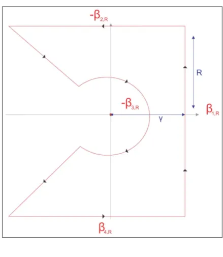
eRe(µ)d|µ|<_∞. Moreover, it is independent of the Hankel’s path chosen. To check this, we start proving that the integral overH ais equivalent to the integral over a parallel line to the imaginary axis, which the elements have the real value bigger thanε. To this end, we first fixγ,R> ε

and consider the pathη_R=β_1,R−β_2,R−β_3,R+β_4,R, where

ηR=

          

β1,R:={γ+i t:t∈[−R,R]}

β2,R:={t+iR:t∈[R/tanθ,γ]}

β_3,R:={z∈H a:_kzk ≤R/sinθ}

β_4,R:={t−iR:t∈[R/tanθ,γ]}

Figure 2.1:

Finite Path

η

_R

Z

ηR

µ−z_eµ

dµ=0

and rewriting, we obtain

Z

β3,R

µ−z_eµ

dµ=

Z

β1,R−β2,R+β4,R

µ−z_eµ

dµ.

Doing a limit process overR, the expression above can be written as

Z

H a

µ−zeµdµ= lim

R→∞

Z

β3,R

µ−zeµdµ= lim

R→∞

Z

β1,R−β2,R+β4,R

µ−zeµdµ.

Therefore, if we show that overβ_2,R and over β_4,R the integrals tends to zero we would obtain the equality

Z

H a

µ−zeµdµ=

Zγ+i∞ γ−i∞

2.1. Tools and special functions 27

Indeed, observe that

Z

β2,R

µ−z_eµ

dµ = Zγ

R/tanθ

e−zlog(t+iR)+(t+iR)d t

≤

Zγ

R/tanθ

et(t2+R2)−Re(z)/2_eIm(z)arg(t+iR)_{d t}

Therefore, we obtain

Z

β2,R

µ−zeµdµ

≤ M

Zγ

R/tanθ

etR−Re(z)d t

=M R−Re(z)

eγ−eR/tanθ

→0, R_{→ ∞}.

So the last computations also allow to prove that the definition of the integral is independent of the Hankel’s path chosen.

Now if we consider t>0fixed by making the substitutionµ=tωin the integral over the curveH a, we obtain

1 2πi

Z

H a

µ−z_eµ

dµ= t

1−z

2πi

Z

H a

µ−z_eµt_dµ= t 1−z

2πi

Zγ+i∞ γ−i∞

µ−z_eµt_dµ.

But we know by the Example 2.6 that ifF(t) =tz−1 then its Laplace transform is

L{F(t)}(µ) =Γ(z)µ−z

and therefore, using the inverse Laplace operator,

1 2πi

Z

H a

µ−zeµdµ= t

1−z

2πi

Zγ+i∞ γ−i∞

µ−zeµtdµ=t1−z_L−1{µ−z}(t) = 1

Γ(z).

ú_THE BETA FUNCTION– We remark that another useful mathematical function in fractional