An Extensive Search for Overtones in Schwarzschild Black Holes
E. Abdalla and D. Giugno Instituto de F´ısica, Universidade de S˜ao Paulo
C.P. 66318, CEP 05315, S˜ao Paulo-SP, Brazil
Received on 2 April, 2007
In this paper we show that with standard numerical methods it is possible to obtain highly precise results for quasi normal modes (QNMs). In particular, secondary modes are obtained by numerical integration done in the well-known null grid. We have compared such numerical results to the also well-known 6th-order WKB method and have found a striking degree of agreement, which could be as good as seven significant figures for the fundamental mode and three for the first overtone. We have chosen the Schwarzschild BH (black hole) to start with because it is the simplest and most well-known of all BHs, so it provides a very safe testing ground to the aforementioned numerical method.
Keywords: Gravitation; Perturbations; Neutron Stars; Quark Stars
I. INTRODUCTION
Wave propagation around black holes is an active field of research (see [1],[2]). The perspective of gravitational wave detection in a near future and the great recent development of numerical general relativity have increased even further the activity on this field [3]. Gravitational waves should be espe-cially strong when emitted by black holes. The study of the propagation of perturbations around them is, hence, essential to provide templates for the gravitational wave identification. A recent challenge has been posed by advances in the black hole merger problem, in which the ringdown phase character-isation from the numerical wave profile is poorly understood, so that the techniques here employed and discussed may be of interest in that context. Thus, activity in this field is develop-ing quickly [1],[4].
The Schwarzschild black hole is very well known [2, 5] but it is important to get reassured about the robustness of the methods and results. Therefore, here, we embark in a detailed study of the secondary modes by means of the subtraction of the first modes in the time domain. The method, though very simple has not been used in the literature due to numerical er-rors intrinsic to the method. However, we were able to use simple standard methods to show that the results are valid im-plying an acuracy of up to seven figures for the dominant (fun-damental) mode and sometimes three for the secondary mode (or first overtone).
In what follows, we have used the geometric system of units, for whichc=G=1. This means that the masses have dimension of length. The conversion factor to CGS/MKS units isc2/G.
II. FUNDAMENTAL MODES AND FIRST OVERTONES
We begin with a series of tables on the frequencies of the QNMs for the Schwarzschild black holes, for the scalar, elec-tromagnetic (EM) and axial gravitational perturbations. We have employed, throughout our discussion,M=1.0, since the Schwarzschild BH frequencies scales asMω=const. For the grid spacing, we have usedh=10−2mthroughout. In what
follows, we have used the notation ωDOM for the dominant mode,ωSEC for the first overtone and, whenever applicable, ωT ERfor the second overtone. We have also listed the quan-titiesδωi,i=DOM,SEC,T ER, which are the estimated er-rors for the corresponding frequency values. Such erer-rors were computed using the method described in detail in the Appen-dix.
Blank spaces, wherever they appear, indicate lack of reli-able data for the mode in question.
Before continuing, a few remarks are due: as expected, the scalar field oscillated very little forℓ=0 compared to higher ℓvalues, so we had to remove its power-law tail numerically (see corresponding note in the Appendix) to get a clearer pic-ture of the corresponding oscillations and then compute its first overtone. The second overtone was not clearly visible for ℓ <6, and even so only forℓ=8 and higher we could perform minimally acceptable fittings on it.
0.0 2.0×101
4.0×101 6.0×101 8.0×101 1.0×10² 1.2×10² 1.4×10² t(m)
10-15 10-14 10-13 10-12 10-11 10-10 10-9 10-8 10-7 10-6 10-5 10-4 10-3 10-2 10-1 100
|W|
n = 0 n = 1 n = 2
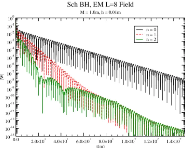
Sch BH, EM L=8 Field
M = 1.0m, h = 0.01m
FIG. 1: Fundamental mode and first overtone, for the electromag-neticℓ=8 field. The second overtone appears very clearly..
The Figs. (1) and (2) show that the second overtone appears clearly only for very highℓ(ℓ >6), and it is the reason why we have blank spaces for this overtone in tables (I) and (II).
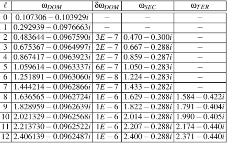
TABLE I: Frequencies for the Schwarzschild BH ofM=1.0 in the case of a scalar field, for differentℓvalues. ℓ ωDOM δωDOM ωSEC ωT ER
0 0.107306−0.103929i − − −
1 0.292939−0.0976663i − − −
2 0.483644−0.0967590i 3E−7 0.470−0.300i −
3 0.675367−0.0964997i 2E−7 0.667−0.288i −
4 0.867417−0.0963923i 2E−7 0.859−0.287i −
5 1.059614−0.0963337i 6E−7 1.050−0.283i −
6 1.251891−0.0963060i 9E−8 1.224−0.283i −
7 1.444214−0.0962866i 7E−7 1.433−0.282i −
8 1.636565−0.0962724i 1E−6 1.629−0.288i 1.584−0.422i 9 1.828959−0.0962639i 1E−6 1.822−0.288i 1.791−0.404i 10 2.021329−0.0962568i 1E−6 2.014−0.288i 1.990−0.405i 11 2.213730−0.0962522i 1E−6 2.207−0.288i 2.174−0.440i 12 2.406139−0.0962487i 1E−6 2.400−0.288i 2.371−0.440i
TABLE II: Frequencies for the Schwarzschild BH ofM=1.0, in the case of an electromagnetic field, for differentℓvalues. ℓ ωDOM δωDOM ωSEC ωT ER
1 0.248229−0.0924905i − − −
2 0.457595−0.0950044i 5E−8 0.440−0.290i −
3 0.656899−0.0956165i 2E−8 0.648−0.286i −
4 0.853096−0.0958605i 2E−7 0.844−0.285i −
5 1.047915−0.0959821i 9E−8 1.039−0.282i −
6 1.242000−0.0960523i 9E−8 1.232−0.282i −
7 1.435647−0.0960959i 7E−7 1.424−0.281i −
8 1.629012−0.0961250i 6E−8 1.621−0.288i 1.577−0.425i 9 1.822180−0.0961452i 1E−6 1.815−0.288i 1.788−0.407i 10 2.015214−0.0961596i 1E−6 2.008−0.288i 1.984−0.410i 11 2.208148−0.0961714i 2E−6 2.199−0.285i 2.164−0.442i 12 2.401004−0.0961800i 1E−6 2.395−0.288i 2.365−0.427i
0.0 2.0×101
4.0×101 6.0×101 8.0×101 1.0×10² 1.2×10² 1.4×10² t (m)
10-14 10-13 10-12 10-11 10-10 10-9 10-8 10-7 10-6 10-5 10-4 10-3 10-2 10-1 100
|W|
n = 0 n = 1 n = 2 (?)
Sch BH, Scalar L=7 Field
M = 1.0m, h = 0.01m
FIG. 2: Fundamental mode and first overtone, for the scalarℓ=7 field. The second overtone also appears, though not in a very evident manner.
When it comes to notation, we have employedℓfor the multi-pole index (as before),nfor the overtone index (n=0 for the fundamental,n=1 for the first overtone, and so on). ωNU M refers to our numerical data, ωW KB1refers to the WKB data
from paper [5] andωW KB2, to paper [6]. We were also able to compare our data to a few data compiled two decades ago by E.W. Leaver, who employed yet another method based on con-tinuous fraction equations. See [7], [8] and references therein. These comparison tables leave no room for doubts when it comes to the fundamental mode,n=0. For all fields and ℓ-values, the data from our numerical simulations and those from the 6th-order WKB method showed a high-degree agree-ment, with differences between 1 part in 104 and 1 part in 105, for bothRe(ω)andIm(ω), especially for higherℓ-values. When it comes to the first overtone, for all fields under study, the agreement between both sets of data was not so impres-sive, hovering around 1−2% forRe(ω)and 2−3% forIm(ω) for lowℓ(typically up toℓ=6) and improving for higherℓ, to a few parts in 1000 forRe(ω)and around 0.5% or so for Im(ω). The second overtone showed much higher discrep-ancies, especially forIm(ω), with differences around 15% is some cases, while forRe(ω) this difference usually hovers around 1−2% (with two exceptions for ℓ=8, when it was much bigger - almost 8% for the axial field).
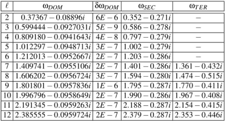
re-TABLE III: Frequencies for the Schwarzschild BH of massM=1.0, in the case of an axial field, for differentℓvalues. ℓ ωDOM δωDOM ωSEC ωT ER
2 0.37367−0.08896i 6E−6 0.352−0.271i −
3 0.599444−0.0927031i 5E−9 0.586−0.278i −
4 0.809180−0.0941643i 4E−8 0.797−0.279i −
5 1.012297−0.0948713i 3E−7 1.002−0.279i −
6 1.212013−0.0952667i 2E−7 1.203−0.286i −
7 1.409741−0.0955106i 2E−7 1.401−0.286i 1.361−0.432i 8 1.606202−0.0956724i 3E−7 1.594−0.280i 1.474−0.515i 9 1.801801−0.0957836i 1E−6 1.795−0.287i 1.770−0.411i 10 1.996796−0.0958649i 2E−7 1.990−0.286i 1.967−0.408i 11 2.191345−0.0959263i 2E−7 2.188−0.287i 2.154−0.415i 12 2.385555−0.0959724i 2E−7 2.379−0.287i 2.353−0.446i
TABLE IV: Frequencies for the Schwarzschild BH ofM=1.0, in the case of a scalar field, for differentℓandnvalues, and their comparison to WKB data.
ℓ n ωNU M ωW KB1 ωW KB2
0 0 0.107306−0.103929i 0.1105−0.1008i 0.1046−0.1152i 1 0 0.292939−0.0976663i 0.2929−0.0977i 0.2911−0.0980i
1 1 − 0.264−0.307i 0.2622−0.3074i
2 0 0.483644−0.0967590i 0.4836−0.0968i 0.4832−0.0968i 2 1 0.470−0.300i 0.4638−0.2956i 0.4632−0.2958i
2 2 − 0.4317−0.5034i 0.4317−0.5034i
3 0 0.675367−0.0964997i 0.675366−0.0965006i −
3 1 0.667−0.288i 0.660671−0.292288i −
4 0 0.867417−0.0963923i 0.867416−0.0963919i −
4 1 0.859−0.287i 0.855808−0.290877i −
5 0 1.059614−0.0963337i 1.05961−0.0963368i −
5 1 1.050−0.283i 1.05004−0.290154i −
6 0 1.251891−0.0963060i 1.25189−0.0963051i −
6 1 1.224−0.283i 1.24375−0.289736i −
7 0 1.444214−0.0962866i 1.44421−0.0962852i −
7 1 1.433−0.282i 1.43714−0.289473i −
8 0 1.636565−0.0962724i 1.63656−0.0962719i −
8 1 1.629−0.288i 1.63031−0.289297i 8 2 1.584−0.422i 1.61797−0.483757i
9 0 1.828939−0.0962639i 1.82893−0.0962626i −
9 1 1.822−0.288i 1.82333−0.289173ii 9 2 1.791−0.404i 1.81225−0.483235i
10 0 2.021329−0.0962568i 2.02132−0.0962558i −
10 1 2.014−0.288i 2.01625−0.289083i 10 2 1.990−0.405i 2.0062−0.482854i
11 0 2.213730−0.0962522i 2.21372−0.0962507i −
11 1 2.207−0.288i 2.20909−0.289015i 11 2 2.174−0.417i 2.19989−0.482567i
12 0 2.406139−0.0962487i 2.40613−0.0962467i −
12 1 2.400−0.288i 2.40186−0.288963i 12 2 2.371−0.440i 2.39338−0.482347i
sult agrees very well with the 6th-order WKB result on both cases. When we looked at the ℓ=3 case for the same per-turbation, Leaver’s results were ω=0.599443−0.092703i whenn=0 andω=0.582644−0.281248iwhenn=1. Our results were 0.599444−0.0927031i and 0.587−0.278i, re-spectively. Again, the agreement between Leaver’s results and ours is excellent for the n=0 mode, but not so good for n=1: ours were higher by about 1% for both Re(ω) and Im(ω). And the 6th-order WKB and Leaver’s results
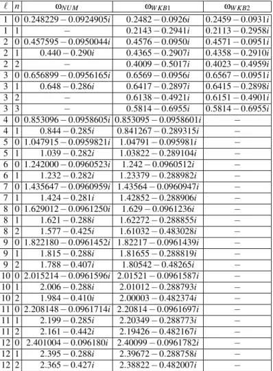
TABLE V: Frequencies for the Schwarzschild BH ofM=1.0, in the case of an electromagnetic field, for differentℓandnvalues, and their comparison to WKB data.
ℓ n ωNU M ωW KB1 ωW KB2
1 0 0.248229−0.0924905i 0.2482−0.0926i 0.2459−0.0931i
1 1 − 0.2143−0.2941i 0.2113−0.2958i
2 0 0.457595−0.0950044i 0.4576−0.0950i 0.4571−0.0951i 2 1 0.440−0.290i 0.4365−0.2907i 0.4358−0.2910i
2 2 − 0.4009−0.5017i 0.4023−0.4959i
3 0 0.656899−0.0956165i 0.6569−0.0956i 0.6567−0.0951i 3 1 0.648−0.286i 0.6417−0.2897i 0.6415−0.2898i
3 2 − 0.6138−0.4921i 0.6151−0.4901i
3 3 − 0.5814−0.6955i 0.5814−0.6955i
4 0 0.853096−0.0958605i 0.853095−0.0958601i −
4 1 0.844−0.285i 0.841267−0.289315i −
5 0 1.047915−0.0959821i 1.04791−0.095981i −
5 1 1.039−0.282i 1.03822−0.289104i −
6 0 1.242000−0.0960523i 1.242−0.0960512i −
6 1 1.232−0.282i 1.23379−0.288982i −
7 0 1.435647−0.0960959i 1.43564−0.0960947i −
7 1 1.424−0.281i 1.42852−0.288906i −
8 0 1.629012−0.0961250i 1.629−0.0961236i −
8 1 1.621−0.288i 1.62272−0.288855i −
8 2 1.577−0.425i 1.61032−0.483028i −
9 0 1.822180−0.0961452i 1.82217−0.0961439i −
9 1 1.815−0.288i 1.81655−0.288819i −
9 2 1.788−0.407i 1.80542−0.48265i −
10 0 2.015214−0.0961596i 2.01521−0.0961587i −
10 1 2.006−0.288i 2.01012−0.288793i −
10 2 1.984−0.410i 2.00003−0.482374i −
11 0 2.208148−0.0961714i 2.20814−0.0961697i −
11 1 2.199−0.285i 2.20349−0.288773i −
11 2 2.161−0.442i 2.19426−0.482167i −
12 0 2.401004−0.096180i 2.40099−0.0961782i −
12 1 2.395−0.288i 2.39672−0.288758i −
12 2 2.365−0.427i 2.38822−0.482007i −
agreement between both sets of results seemed to be beyond any doubt to us.
In short, from the few data we have from Leaver’s work, we might say that Leaver’s data seem to be more precise for the Schwarzschild case. Our method, however, may be useful when the perturbative potentials are too awkward or compli-cated to conform to an analytic or semi-analytic method of computing quasinormal frequencies, so that direct numerical integration remains the sole option for that goal.
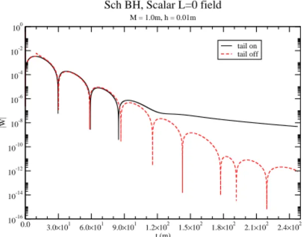
A brief remark is due on the scalarℓ=0 case. As we had already pointed out in this text, we had to subtract the power-law tail from the original field, so that we could have a suf-ficent number of oscillations to render any frequency fitting meaningful. For that particular case, however, the agreement between our data and 6th-order WKB was not perfect, since we gotω=0.107306−0.103929i, while the 6th-order WKB result wasω=0.1106−0.1008i, that is, a discrepancy of 3% forRe(ω)and 7% forIm(ω). See Fig. (3).
APPENDIX A: ON THE NUMERICAL METHOD FOR OBTAINING THE WAVE PROFILES
We provide here a brief sketch of the method employed to find the wave profiles - let the grid in which the method oper-ates be calledx−t grid- from which we have later extracted the dominant mode and the overtones - the latter theme will be thoroughly treated in the next section.
TABLE VI: Frequencies for the Schwarzschild BH of massM=1.0, in the case of an axial field, for differentℓandnvalues, and their comparison to WKB data.
ℓ n ωNU M ωW KB1 ωW KB2
2 0 0.37367−0.08896i 0.373691−0.088891i 0.3732−0.0892i 2 1 0.352−0.272i 0.346297−0.27348i 0.3460−0.2749i
2 2 − 0.2985−0.4776i 0.29852−0.47756i
3 0 0.599444−0.0927031i 0.599443−0.0927025i 0.5993−0.0927i 3 1 0.587−0.278i 0.582642−0.28129i 0.5824−0.2814i 3 2 − 0.551594−0.479047i 0.5532−0.4767i 4 0 0.809180−0.0941643i 0.809178−0.0941641i 0.8091−0.0942i 4 1 0.797−0.279i 0.796631−0.284334i 0.7965−0.2844i
4 2 − 0.7727−0.4799i 0.772695−0.4799i
5 0 1.012297−0.0948713i 1.0123−0.0948706i −
5 1 1.002−0.279i 1.00222−0.285817i −
6 0 1.212013−0.0952667i 1.21201−0.0952659i −
6 1 1.203−0.286i 1.20357−0.28665i −
7 0 1.409741−0.0955106i 1.40974−0.0955096i −
7 1 1.401−0.286i 1.40247−0.287164i −
7 2 1.361−0.432i 1.38818−0.480709i −
8 0 1.606202−0.0956724i 1.60619−0.0956707i −
8 1 1.594−0.280i 1.59981−0.287504i −
8 2 1.474−0.515i 1.58721−0.480804i −
9 0 1.801801−0.095784i 1.80179−0.0957828i −
9 1 1.795−0.288i 1.7961−0.287741i −
9 2 1.770−0.440i 1.78483−0.48087i −
10 0 1.996796−0.0958649i 1.99679−0.0958639i −
10 1 1.990−0.286i 1.99165−0.287912i −
10 2 1.967−0.408i 1.98145−0.48087i −
11 0 2.191345−0.0959263i 2.19133−0.0959245i −
11 1 2.185−0.287i 2.18665−0.28804i −
11 2 2.154−0.415i 2.17734−0.480952i −
12 0 2.385555−0.0959724i 2.38554−0.095971i −
12 1 2.379−0.287i 2.38124−0.288138i −
12 2 2.353−0.446i 2.37268−0.480979i −
one may evolve the fieldΨin time via Ψ(t0+δt,x0) =
− Ψ(t0−δt,x0) + (2−δ2xV(x 0)−
5δt2
2δx2)Ψ(t0,x0) + + 4δt
2[Ψ(t0,x0+δx) +Ψ(t0,x0−δx)]
3δx2 −
− δt
2[Ψ(t0,x
0−2δx) +Ψ(t0,x0+2δx)]
12δx2 . (A1)
In the prescription (A1), one computes the fieldΨat(x,t) = (x0,t0+δt)from the values of the field at 5 different points at the instantt0and from the value of the field in one point at the instantt0−dt. At the initial instanttini, one specifies not only Ψ, but also∂Ψ
∂t, for the whole spatial rangexini<x<xf in. The very structure of (A1) causesxmaxto increase by 2δxandxmin to decrease by the same amount - the algorithm develops in time like an inverted cone - and the integration stopped for a predetermined value oft(or time steps). An illustration of the method is provided in Fig. (A).
A point of paramount importance is to be stressed for the current method: the time spacingδt must be always smaller in magnitude than the spacing inx,δx. That is, ifm=δt
δx <1.
This is necessary to preserve numerical stability. Thismis calledmesh ratio.
As for the initial conditions in use, they make little differ-ence in the final result, since we are interested in the quasi-normal ringdown of the fields, which do not depend on the initial condition. We have used an initial Gaussian pulse of unit magnitude centered atx=0, due to its ease of implemen-tation.
APPENDIX B: FINDING THE OVERTONES NUMERICALLY
0.0 3.0×101
6.0×101 9.0×101 1.2×10² 1.5×10² 1.8×10² 2.1×10² 2.4×10² t (m) 10-16 10-14 10-12 10-10 10-8 10-6 10-4 10-2 100 |W| tail on tail off
Sch BH, Scalar L=0 field
M = 1.0m, h = 0.01m
FIG. 3: Fundamental mode with and without tail, for the scalarℓ=0 field. Notice how the oscillations are masked by the power-law tail.
✻
✲
t
x
Ψ(t=0), ˙
Ψ(t=0) ❅ ❅ ❅ ❅ ❅ ❅ ❅ ❅ ❅ ❅ ❅ ❅ ❅ ❅
Ψ(t+δt)
Ψ(t)
Ψ(t−δt)
tmax
x
x
x x
x x x
u u
u u
u
u u
u u u u u u u u u u
u u u u
u u u
u u u u u u
u u u
u u u u
u u u
FIG. 4: Thex−tgrid.
how do we recognize the dominant mode, since the overtones also contribute to the wave profile ?
The answer is that we expect the overtones to decay much faster than the dominant mode, so that their contribution shows up at the early stages of the waveform (transient part and the early ringdown phase). Hence the late-time ringdown phase is completely dominated by this n=0 mode, and the aforementioned quantities A,ωI,ωR are taken at this phase. The reader, upon looking again at the Figs. (1) and (2), will be convinced that this is indeed the case.
These data on then=0 mode were taken with the max-imum number of significant digits possible (usually 8 or 9), and we subtracted the fitted function from the original wave profile. That fitted function had the form
Ψ0=Aexp(iω0
Rt)exp(−ω0It), (B1) so that we could see the remainder of this operation.
In all cases (except for theℓ=0,1 scalar andℓ=1 EM field), after performing the subtraction above, we could find a
remainder of the form ΨR=Bexp(iω1
Rt)exp(−ω1It) +∆, (B2) in whichω16=ω0, characterizing a secondary mode (the first overtone), and with similar amplitudes (A≈B). The term∆
is just theΨ0 term, but with a much reduced amplitude, in-dicating that the fitting operation has its precision limitations. This can be seen in the form of parallel curve envelopes in the Figs. (1) and (2), for example. Needless to say, we picked the n=1 mode fitting data at the end of its own quasinormal ring-ing phase, for the same reasons outlined above for then=0 mode.
A similar procedure was adopted to find the second tone, this time applying the oscillatory fitting to the first over-tone, in which a new remainder similar to that seen in (B2) was seen. In this latter case, however, only the very high ℓ-values could yield any valuable result when an oscillatory fitting was applied to it. This is directly related to the de-gree of precision to which we could find the amplitude and the frequenciesωR andωI: since the number of significant figures for them was around 3. Less significant figures trans-late into greater errors in the subtraction process to find the tertiary mode, which in turn translates into somewhat blurred wave profiles for that tertiary mode. Another difficulty in-volved in finding it is that it decays much faster than then=0 andn=1, which means it is available for extraction only at the very early stages of the original waveform. This very re-duced time interval for mode extraction compromises the os-cillatory fitting quality and is responsible for then=1 mode’s much lower number of significant figures when compared to then=0 mode, since then=2 mode is used to estimate the n=1 mode’s fitting precision.
The fact that in some cases we cannot see then=1 mode can be easily explained: these cases correspond to very low values forℓ, namelyℓ=0,1, for which very few oscillations appear even for the dominant mode, thus rendering it very difficult, if not impracticable, to extract an overtone from the corresponding wave profiles. Then=2 mode, in turn, is usu-ally only detectable for higher values ofℓ(ℓ >6). We are still figuring out why this happens.
Now it is the time to estimate the precision of the first fit-ting. As we can see again in the aforementioned figures, there is a given timetcfor which the secondary mode and the dom-inant mode are roughly equal in magnitude, that is
Bexp(iω1
Rt)exp(−ω1It)≈δ(Aexp(iω0Rt)exp(−ωIt)). (B3) The variation of the dominant mode can be expressed as
δ(Aexp(iω0
Rt)exp(−ωIt)) = (δA)exp(iω0Rt)exp(−ωIt) + + Aiexp(iωRt)exp(−ωIt)[δω0
R+iδω0I]t. (B4)
In what follows, we assumeδAto be much smaller thanA. Such approximation implies
Bexp(iω1
Rt)exp(−ω1It)≈Aitδωexp(iω0R)exp(−ω1It), (B5) in which we have usedδω=δω0
R+iδω0I.Working with the moduli of the quantities above, we arrive at
|δω|≈|B A|
exp(−[ω1 I−ω0I])t
Upon substitutingt=tcand noting that|A|≈|B|, we arrive at
|δω|≈exp(−[ω 1
I−ω0I])tc tc
. (B7)
Such an estimate was done for each field and for eachℓ-value, and|δω|was compared to|ω|, so as to determine the approx-imate degree of precision in the computation of the dominant mode frequency. A similar estimate can also be done, in prin-ciple, for the first overtone fitting precision. We have deter-mined the ratiom=|δωω|- for then=0 mode - to be smaller than 10−6, in all cases we have dealt with, except for the axial ℓ=2 case, for whichm≈10−5(hence its smaller number of
significant figures).
A final remark is needed for the scalar field, in theℓ=0 case. Since this particular field decays as a power-law tail quite soon in the time domain (compared to higherℓfields), we had to perform a law fitting (the classical power-law tail of the fields evolving in a Schwarzschild spacetime) on its tail and then subtract it from the original mode, there-fore unveiling oscillations decaying beneath the tail, as al-ready seen in Fig. (3). The numerical unveiling of its first overtone was then tried in the same way as in all the remain-ing fields, though we failed to get a clear picture of it, for the reasons described earlier in this Appendix.
[1] F. Pretorius, Phys. Rev. Lett.95, 121101 (2005).
[2] T. Regge and J. A. Wheeler, Phys. Rev.108, 1063 (1957); S. Chandrasekhar,The Mathematical Theory of Black Holes, (Ox-ford University Press, Ox(Ox-ford, 1983); K. D. Kokkotas and B. G. Schmidt, Living Rev. Relativity2(1999).
[3] O.D. Aguiar et al., Class. Quant. Grav. 23, S239 (2006). [4] R. Price, Phys. Rev. D5, 2419 (1972); C. Gundlach, R. Price,
and J. Pullin, Phys. Rev. D49, 883 (1994); V. Cardoso and J. P. S. Lemos, Phys. Rev. D64, 084017 (2001); Bin Wang, Chi-Yong Lin, and Elcio Abdalla Phys. Lett. B481(2000) 79; Bin Wang,
C. Molina, and Elcio Abdalla Phys. Rev. D63, 084001 (2001); C. Molina, D. Giugno, E. Abdalla, and A. Saa, Phys. Rev. D69, 104013 (2004); R. A. Konoplya, A. V. Zhidenko Phys. Lett. B
609, 377 (2005); E. Abdalla, B. Cuadros-Melgar, A. B. Pavan, and C. Molina Nucl. Phys. B752, 40 (2006).
[5] R. A. Konoplya, J. Phys. Stud.8, No. 1, 93 (2004). [6] S. Iyer, Phys. Rev. D35, 12, 3632 (1987).