A Dynamic Model for the Analysis of
Surge in a Tropical Storm
Alexis Amezaga-Hechavarra
1, Jose Marn-Antu~na
2, Manuel Tejera-Fernandez
3and
Julio Navarro-Serrano
4 1Group of Theoretical Physics, ICIMAFCalle E#309, esq. a 15, CP 10400 Ciudad Habana, Cuba,
2Faculty of Physics, University of Havana
San Lazaro y L, Habana, Cuba,
3Department of Physics, IPSJAE, Marianao, Habana, Cuba,
4Department of Nautic Research, GEOCUBA, Calle 4,#304, Playa, Habana.
Received 12 November, 1998; Revised 22 March, 1999
We obtain an analytic representation for the prole of the surge wave in the sea, due to a tropical storm at a low latitude. The results reproduce the known experimental data adequately. In the calculations we take into account the inuence of Rossby's second parameter and we analyse its contribution to the surge wave, which is proved to be suciently small to be neglected in higher latitudes. The obtained analytical solution allows us to study in detail the surge wave formation in the presence of such a storm. To solve the problem, Laplace method and Green functions are used. This allows us to improve previous results obtained by Evsa in 1989.
I Introduction
In the last years the interest of studying non-periodic oscillations of sea level has grown. In particular, it is of interest the study of those oscillations excited by pres-sure elds and strong winds in the tropical storm. It is possible to nd previous information about this theme in the work of Jelesniansky [1] and more recently, Johns et al. [2], Fandry et al. [3], Jerome et al. [4], Signorini [5], Davies et al. [6] and Lardner et al. [7] and [8]. The majority of these papers employ numerical methods or qualitative analysis of the solution of the mathematical model. In the present paper we obtain an analytic so-lution of the problem, similar to the one formulated by Evsa [9]. In this work, there is an incorrect expresion for the Green function of the problem. Therefore, for the analytic solution, Evsa does not take account of the multi-valuated character of the complex variable func-tion in the path integrafunc-tions. In the present paper we make correct use of the Green function method and the integral transform techniques. We also analyze the in-uence of Rossby's second parameter, which is usually
neglected at high latitudes by other authors because of its smallness with respect to Rossby's rst parameter and because it allows to simplify the calculation. We check that Rossby's second parameter is small enough to be neglected at low latitudes.
II Formulation of the problem
Let us consider a tropical cyclone (TC) which causes a perturbation of the sea surface in an ocean region distant from any coast. The interaction region has a characteristic deepness less than the storm horizontal size by two orders of magnitude. Therefore, we can use the shalow water approximation. We also consider a quasistationary regime for the storm, in order to keep a xed coordinate center. Due to the axial symmetry of this problem, we use a cylindrical system of coordinates with center on the axis of the cyclone.
The Navier-Stokes equations in the cilindrical sys-tem of coordinates including the Coriolis terms are given by
c @u
+u @u
+v@u
+w @u
, v
2
=fv,f
w,
1@P a
+ 1@ r z
@v @t
+u @v @r
+v r
@v @'
+w @v @z
, uv
r
=,fu,
1
1
r @P
a @'
+ 1
@
'z @z
; (2)
@w @t
+u @w
@r
+v r
@w @'
+w @w
@z
=f
u,
1
@P
a @z
,g ; (3)
d
with u = v r,
v = v ',
w = v z,
f = 2sin, f
=
2cos. Here is the angular Earth velocity andis
the latitude of the region under consideration.
In these equations the term of the divergence of the stress tensor contains only the vertical stress forces be-cause they are much larger than the rest of the internal friction eects. In equation (3), all the stress eects are neglected in comparison with the vertical pressure gradient and with the gravity acceleration.
The equation of continuity in cylindrical coordinates is
@u @r
+ 1
r @v @'
+@w @z
+u r
= 0: (4)
The bondary conditions are: in the botton, the ad-herence condition; at the sea surface, the kinematic con-dition (w j
z == d dt
u @ @r +
v r
@ @'+
@ @t).
The Oz axis coincides with the external normal vec-tor to the Earth surface. We also suppose the integra-tion time in these equaintegra-tions is much smaller than the cyclone displacement characteristic time. Therefore, we take into account the time derivatives, although we con-sider the TC static.
By integration of equation (1)-(3) along the z direc-tion, we obtain the following system, for the shallow water approximation, in dimensionless form,
c
St ,1
@u @t
+ (+h) @P
a @r
+Fr ,1(
+h) @ @r
,Ro ,1
v+Ro ,1
Z ,h
w dz= s r
, f r
; (5)
St ,1
@v @t
+ (+h) r
@P a @'
+Fr ,1(
+h) r
@ @'
+Ro ,1
u= s '
, f '
; (6)
St ,1
@ @t
+@u @r
+ 1
r @v @'
+u r
= 0 : (7)
d
We neglect the convective acceleration terms, be-cause the absence of coasts implies that the velocity gradients are very small in the considered region. In the above equations is the sea perturbation average
level; h is the non-perturbed sea deepness; P
a is the
atmospheric pressure eld originated by the TC; s i
are the surface stresses produced by the TC winds and
s
i are the bottom stresses (
i = r;');
0 is the water
density;H is the characteristic deepness of the region; St= (U
0
T)=Lis the Struhal's number;Fr=U 2 0
=(g H)
is Froude's number;R 0=
U 0
=(fL) is Rossby's rst
pa-rameter andR 0=
U 0
=(f
H) is Rossby's second
param-eter; U
0 is the characteristic velocity;
L is the
charac-teristic size on the horizontal ocean surface plane. We take 5
because the contribution of f
is bigger at
very low latitudes. This is precisely the interest of our study, maintainingf not equal to zero in the model.
In the following calculation we neglect b
i because
the processes are essentially supercial and therefore the bottom does not matter. Also, we consider+h h= 1 because in the problem hand that the
prob-lem is axisymmetric so that @[::] @'
0. The presence of
Rossby's second parameter in equation (5) makes it im-possible to use the two-dimensional approach employed by other authors. To avoid this problem, we assume an exponential dependence of the horizontal velocities with respect to the vertical coordinate,
u(r;';z;t) = u 0(
r;';t)exp[,a(,z)]; v(r;';z;t) = v
0(
r;';t)exp[,a(,z)]:
We take an exponential dependence because, in many uid problems, that is the law of variation of the hori-zontal velocities with respect to the deepness and con-sidering the gravity constant in the studied region. This assumption is consistent with our model, in which Fr
is constant:
With this dependence we have that, at the surface
z=; velocities areu 0 and
v
0. The parameter a
con-trols the decrease of the velocities withz. Expressions
(8), using (4), allow us to obtain
c Z
,h
wdz=H
u @ @r
+v r
@ @'
,
H a
@u @r
+ 1
r @v @'
+u r
: (9)
We have neglected the convective derivative of in the rst term because the calculations are made in open
sea [10], [11] and also because we only consider the long wave generated by TC. Hence (H= 1, the dimensionless
formulation)
= 1
a
@u @r
+u r
:
1 (10)
Then, system (1),(3) takes the form
St ,1
@u @t
+@Pa @r
+Fr ,1
@ @r
,Ro ,1
v+Ro ,1
= s r
; (11)
St ,1
@v @t
+Ro ,1
u= s '
; (12)
St ,1
@ @t
+@u @r
+u r
= 0: (13)
d
To solve this system we consider homogeneous ini-tial conditions and the following boundary conditions,
uj r !1=
v j r !1=
j
r !1= 0
; j
r =0 <M :
(14) To accomplish the calculations we take, following Johns et al. [2],
s r =
0sin
2(
r), s '=
0cos
2(
r),
where 0 =
1
2 1
W 2 0 and
(r) = 2(r =R)=[1 + (r =R) 2].
Here
1 is the density of the air,
1 is the drag
coe-cient, Wo is the wind velocity in the radius R of the
greatest winds, andis the uency angle of the wind
in the TC. We take the following dependence for the at-mospheric pressure Pa(r) =P
1
,P=[1 + (r =R) 2]1=2
in correspondence with the common assumption in the studies of surge in tropical storms (see, for instance, [1, 11]).
III Calculation
In the system of equations (11)-(13),"(Ro ),1
1.
Hence, we assume an analytic dependence of the
solu-tionu,v, (see e.g. [12]),
u(r;';t) = 1 P n=0
u n(
r;';t)" n
; (15)
v(r;';t) = 1 P n=0
v n(
r;';t)" n
; (16)
(r;';t) = 1 P n=0
n(
r;';t)" n
: (17)
Substituting (15),(16) into equations (11),(13)
and taking only the two rst terms of the sequenceu 0, v
0,
0, and u
1, v
1,
1, we obtain the following systems:
1If directly we shall take a linear variation of the vertical velocity, for instance,
w= (1 +z =H)(d =dt), it simply shall give another
c -Zero-order system St ,1 @u 0 @t
+@Pa @r
+Fr ,1 @ 0 @r ,Ro ,1 v 0= s r ; (18) St ,1 @v 0 @t +Ro ,1 u 0= s ' ; (19) St ,1 @ 0 @t +@u 0 @r +u 0 r
= 0 ; (20)
-First-order system. St ,1 @u 1 @t + 1 @Pa @r
+Fr ,1 @ 1 @r ,Ro ,1 v
1+ 0= 0
; (21) St ,1 @v 1 @t +Ro ,1 u 1= 0
; (22) St ,1 @ 1 @t +@u 1 @r +u 1 r
= 0 : (23)
In our case, it is sucient to take the solution at rst order in perturbation theory, because the small parameter
" in (11) is multipliying a term which is of a very small order, due to the smoothness of the used model. This
fact leads to a non-singular perturbation problem. Hence, (15),(17) are, not only asymptotic, but also monotonic
expansions. We apply the Laplace transform to system (18),(20). For E 0(
r;p) = Lf 0(
r;t)g we obtain the
following equation 1 r d dr r dE 0 dr ,R p E o= Fr
@F(r;p) @r
, F(r;p)
r
; (24)
where F(r;p) = F 1(
r;p),(St=pRo)F 2(
r;p), F 1(
r;p) = [ 0sin
2(
r)-@Pa=@r]=p, F 2(
r;p) = 0cos
2(
r)=p, R p= (p 2+ 2),
=Fr =St 2,
=St=Roandp=s+i.
We can express the solution of equation (24) as
E 0(
r;p) =Fr 1 Z 0
G(r;s)
@F(s;p) @s
, F(s;p)
s
ds; (25)
where
G(r;s) = 8 > > > > > > > < > > > > > > > : I 0 ( p R p r ) I0( p RpR1) I 0( p R p R 1) K 0( p R p s),I
0( p
R p
s)K 0( p R p R 1) ;
0rs<R 1 I0( p Rps) I 0 ( p R p R 1 ) I 0( p R p R 1) K 0( p R p r),I
0( p
R p
r)K 0( p R p R 1) ;
0sr<R 1
(26)
is the Green function of the operator of equation (24), which satises the boundary conditions G(r;s)j r =0
<M; G(r;s)j
r !1= 0; R
1; R
1is the TC external radius.
The inverse Laplace transform gives
0(
r;t) = r R 0 1 2 i a+i1 R a,i1
G(r;s) h A 1 (s) p + A 2(
s)p 2
i
exp(pt)dpds
+ R1 R r 1 2 i a+i1 R a,i1
G(r;s) h
A1(s)
p +
A 2(
s)p 2
i
exp(pt)dpds;
(27)
A 1(
s) = Fr 0sin
(s) [2@(s)=@s,(s)=s]+
@ 2
Pa=@s 2
,@Pa=@s
; A
2(
s) = (Fr St=R o)
0cos
(s)[(s)=s,2@(s)=@s] : (28)
Usual techniques of the theory of functions of complex variables allow us to calculate the contour integrals in (27). We obtain
0(
r;t) = 2 pi
4 X i=1 I
i
; (29)
where
I 1 =
r Z 0
Z 0
G(r;s) A
1(
s)sin(t)
dds; (30)
I 2 =
r Z 0
Z 0
G(r;s) A
2(
s)(1,cos(t)
2
dds; (31)
I 3 =
R1 Z r
Z 0
G(r;s) A
1(
s)sin(t)
dds; (32)
I 4 =
R 1 Z r
Z 0
G(r;s) A
2(
s)(1,cos(t)
2
dds: (33)
In similar form we apply the Laplace transform to system (21)-(23) and obtain for E 1(
r;p) =Lf 1(
r;t)gthe
equation
1
r d dr
r
dE 1 dr
,R
p E
1= F
r
@F(r;p) @r
,F(r;p)
; (34)
where
F(r;p) = pE
0( r;p) aSt
: (35)
The solution of (34) is
E 1(
r;p) =Fr Z
R1 0
G(r;s)
@F(s;p) @s
,F(s;p)
ds: (36)
We proceeded as in the above zero order case in order to obtain 1(
r;t). The results are
1(
r;t) = 2
4 X j=1
2 X i=1
(A j i+
B j i)
; (37)
where A j i and
B j
i are given in the appendix.
d
IV Results and Discussion
We have obtained an analytic representation for the prole of the surge wave in the sea due to a TC at low latitude, given by
(r;t) = 0(
r;t) +" 1(
r;t); (38)
where 0and
1are given by (29) and (37), respectively.
As it can be seen, these expresions present
di-culties to analyse the main properties of the solution. However, they allow checking the analitical dependence with respect to model input parameters. The obtained dependence shows that the expression is stable with re-spect to any continued variation of the corresponding parameter.
between the obtained solution and the experimental data. The values of the parameters are the following: t = 0:5;1;:::;4 hours, R = 50 Km, W0 = 38 m/s, 1 =
0:0025, p = 55 mBar, = 10
, = 1:293 Kg=m3,
St = 0:01, R0 = 0:79, = 0:14 and Fr = 0:0001. We
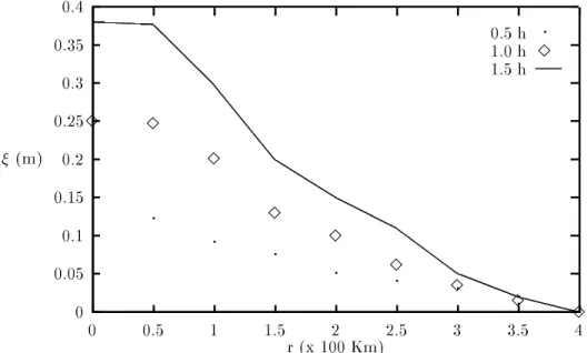
elaborate graphs of sea excitation vs. TC radius. From Figs. 1, 2 and 3, it can be seen the dynamics of the surge wave formation. The plots show that the solution qualitatively maintains its form during time and that it smooth.
0 0.05 0.1 0.15 0.2 0.25 0.3 0.35 0.4
0 0.5 1 1.5 2 2.5 3 3.5 4
(m)
r (x 100 Km)
0:5 h 1:0 h 3
3
3
3
3
3
3
3
3
3
1:5 h
Figure1. Prolesofthesurgewavefort=0.5,1.0and1.5hours.
0 0.1 0.2 0.3 0.4 0.5 0.6 0.7 0.8 0.91
0 0.5 1 1.5 2 2.5 3 3.5 4
(m)
r (x 100 Km)
3:5 h 4:0 h 3 3
3
3
3
3
3
3
3
3
Figure 3. Proles of the surge wave for t=3.5 and 4.0 hours.
3 4 5 6 7 8 9 10 11
0 20 40 60 80 100 120 140 160 180
(m)
Time (h)
'FIG4.DAT' 3
3 3
3 3
3 3
3 3
3 3
3 3
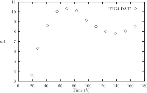
Figure 4. Evolution in time of the surface excitation in r=0.
Table 1. Contribution of the second Rossby parameter to the surface excitation in r=0 for several times. Excitation (r = 0) t = 1 h t = 2 h t = 3 h t = 4 h
0 (m) 0:255 0:510 0:764 1:020
= 0+ "1 (m) 0:257 0:512 0:766 1:023
In Fig. 4 a second experiment shows that the so-lution tends to a bounded oscillatory expression as the time t increases. It is necessary to say that the limit values of the excitation in this case do not correspond
In Table 1, we show the result of another experiment in which it can be seen the real contribution of Rossby's second parameter, i.e. the contribution to the surface excitation, due to the horizontal streams caused by the deection of the vertical internal streams into the sea as a result of the Earth rotation.
It can be seen that this contribution is small, due to the fact that the vertical streams are quite small in comparison with the horizontal streams induced by the wind of the TC. Moreover, the relative increase of the term in the equation containing Rossby's second pa-rameter with respect to the term that contains Rossby's rst parameter is due to the abrupt decrease of the lat-ter. Hence, it is possible to neglect the contribution of
Rossby's streams even at low latitudes.
We have obtained an analytical expression of the excitation of the sea level in the presence of a tropi-cal cyclone, whose results are similar to those obtained by numerical methods. The analytical solution allows us to study in detail the surge wave formation in the presence of a tropical cyclone. It is possible to see that a non-periodical wave is obtained which tends to some stationary state. It is interesting to highlight that the contribution of Rossby's second parameter is quite small even in low latitudes. This result justies the di-rect use of the two-dimensional system of order zero to calculate the surge.
c
Appendix
Expresions for the coecientsA j i and
B j
i in formula (37).
A 1 1 = r Z 0 s Z 0 Z 0 G 1(
s)G 2( r) G 2( s) s G 1(
y)A 1(
y)cos (t)ddy ds (39)
A 2 1 = r Z 0 s Z 0 Z 0 G 1(
s)G 2( r) @G 2( s) @s G 1(
y)A 1(
y)cos(t)ddy ds (40)
A 3 1 = r Z 0 R1 Z s Z 0 G 2(
r)G 1( s) G 1( s) s G 2(
y)A 1(
y)cos(t)ddy ds (41)
A 4 1 = r Z 0 R 1 Z s Z 0 G 2(
r)G 1( s) @G 1( s) @s G 2(
y)A 1(
y)cos(t)ddy ds (42)
B 1 1 = R1 Z r s Z 0 Z 0 G 1(
r)G 2( s) G 2( s) s G 1(
y)A 1(
y)cos(t)ddy ds (43)
B 2 1 = R 1 Z r s Z 0 Z 0 G 1(
r)G 2( s) @G 2( s) @s G 1(
y)A 1(
y)cos(t)ddy ds (44)
B 3 1 = R 1 Z r R 1 Z s Z 0 G 1(
r)G 2( s) G 1( s) s G 2(
y)A 1(
y)cos(t)ddy ds (45)
B 4 1 = R1 Z r R1 Z s Z 0 G 1(
r)G 2( s) @G 1( s) @s G 2(
y)A 1(
y)cos(t)ddy ds (46)
A 1 2 = r Z s Z Z G 1(
s)G 2( r) G 2( s) s G 1(
y)A 2(
y)sin( t)
A 2 2 = r Z 0 s Z 0 Z 0 G 1(
s)G 2( r) @G 2( s) @s G 1(
y)A 2(
y)sin( t)
ddy ds (48)
A 3 2 = r Z 0 R1 Z s Z 0 G 1(
s)G 2( r) G 1( s) s G 2(
y)A 2(
y)sin( t)
ddy ds (49)
A 4 2 = r Z 0 R 1 Z s Z 0 G 1(
s)G 2(
r)G 1(
s)G 2(
y)A 2(
y)sin( t)
ddy ds (50)
B 1 2 = R1 Z r s Z 0 Z 0 G 1(
r)G 2( s) G 2( s) s G 1(
y)A 2(
y)sin( t)
ddy ds (51)
B 2 2 = R1 Z r s Z 0 Z 0 G 1(
r)G 2( s) @G 2( s) @s G 1(
y)A 2(
y)sin( t)
ddy ds (52)
B 3 2 = R 1 Z r R 1 Z s Z 0 G 1(
r)G 2( s) G 1( s) s G 2(
y)A 2(
y)sin( t)
ddy ds (53)
B 4 2 = R 1 Z r R 1 Z s Z 0 G 1(
r)G 2( s) @G 1( s) @s G 2(
y)A 2(
y)sin( t)
ddy ds (54)
and
G 1(
x) = I 0( x p 2 ,
2) (55)
G 2(
x) = K 0( x p 2 , 2) , K 0( R 1 p 2 , 2) I 0( R 1 p 2 , 2) I 0( x p 2 ,
2) (56)
A 1(
y) = H Fr 2 aSt 0sin
(y)
(y) y
,2 @(y)
@y + @ 2 Pa @y 2 , 1 y @Pa @y (57) A 2(
y) = HSt 2 a 0cos (y)
2@(y) @y
, (y)
y
; (58)
where a= 100 and H= 1.
d
Acknowledgments
We want to express our gratitude to the Department of Theoretical Physics of the University of Havana; to the colleagues of the IV Congress of Applied Mathematics in Vic, Barcelona, Spain, in September 1995; to col-leagues of the University of Zaragoza and of UNED in Madrid, to Dr. P. Ripa from CICESE in Mexico, for a great interest in our work, and to Prof. A. Li~nan from the Aeronautical Institute of Madrid, Spain, for fruitful discussions and comments. JMA wants to acknowledge the support of the Alma Mater grant to his research project.
References
[1] C.P. Jelesniansky, Monthly Weather Rev., 98, 472
(1970).
[2] B. Johns, Q. JLR. Met. Soc.,109, 211 (1983).
[3] C. B. Fandry, Dt. hidrogr Z42, 307 (1989).
[4] P. Jerome, Coastal Engineering,14, 1 (1990).
[5] S. R. Signorini, J. Geophys. Res.,97, 2229 (1992).
[6] A. M. Davies and J. E. Jones, Cont. Shelf Res.,12,
[7] R. W. Lardner, P. Smoczynski, Proc. R. Soc. of London A,430, 263 (1990).
[8] R. W. Lardner, A. H. Al-Rabch, N. Gunay, Geophys. Res.,98,c10, 18229 (1993).
[9] N. S. Evsa, Meteor. I Guidrol., 3, 74 (1989).
[10] S. Pond and G. L. Pickard, Introductory Dynamical
Oceanography, Pergamon Press, Oxford (1983). [11] B. Johns, Physical Oceanography of Coastal and Shelf
Seas, Elsevier Publisher, Amsterdam (1983).