www.ann-geophys.net/30/163/2012/ doi:10.5194/angeo-30-163-2012
© Author(s) 2012. CC Attribution 3.0 License.
Annales
Geophysicae
Direct observations of the formation of the solar wind halo from
the strahl
C. Gurgiolo1, M. L. Goldstein2, A. F. Vi ˜nas2, and A. N. Fazakerley3 1Bitterroot Basic Research, Hamilton, Montana, USA
2Geospace Science Laboratory, Code 673, NASA Goddard Space Flight Center, Greenbelt, MD, USA
3Mullard Space Science Laboratory, University College London, Holmbury St. Mary Dorking, Surrey RH5 6NT, UK Correspondence to:C. Gurgiolo ([email protected])
Received: 25 July 2011 – Revised: 12 November 2011 – Accepted: 18 December 2011 – Published: 17 January 2012
Abstract. Observations of a continual erosion of the strahl and build up of the halo with distance from the sun suggests that, at least in part, the halo may be formed as a result of scattering of the strahl. This hypothesis is supported in this paper by observation of intense scattering of strahl electrons, which gives rise to a proto-halo electron population. This population eventually merges into, or becomes the halo. The fact that observations of intense scattering of the strahl are not common implies that the formation of the halo may not be a continuous process, but one that occurs, in part, in bursts in regions where the conditions responsible for the scattering are optimum.
Keywords. Interplanetary physics (Solar wind plasma; Sources of the solar wind) – Space plasma physics (Wave-particle interactions)
1 Introduction
The solar wind has been studied for more than 40 years and while most of the major processes involved in the formation and expansion of the wind are reasonably understood there are still details that need to be worked out. For a detailed discussion an excellent set of comprehensive reviews on the solar wind can be found in Marsch (2006) and Bruno and Carbone (2005). The electron component of the solar wind consists of four distinct populations; a thermal core and a su-perthermal halo (Feldman et al., 1975), a superhalo which is a halo-like population beginning about 2 keV and extending upwards to about 100 keV Lin (1998), and the field-aligned strahl (Rosenbauer et al., 1976, 1977). Models and simula-tions indicate that the electron solar wind is formed within the solar corona (e.g., see Vocks and Mann, 2003; Vocks et al., 2005, 2008) through a combination of wave-particle interactions and Coulomb collisions. It is not clear if on
es-caping the corona either the halo or strahl are distinct popula-tions but they are certainly distinct and identifiable by 0.3 AU (Pilipp et al., 1987a,b,c; ˇStver´ak et al., 2009).
As the solar wind propagates away from the sun, the mir-ror force should focus the strahl in pitch-angle. Observa-tions, however, show it to actually broaden with radial dis-tance (Pilipp et al., 1987b,c; Hammond et al., 1996), indi-cating that there is some interaction between it and the lo-cal plasma. The broadening begins where scattering would be expected to dominate over focusing (Owens et al., 2008), however, the source(s) of the scattering are, as yet, unknown. A possible source is a resonant interaction of the strahl with sunward propagating whistler waves (e.g., see Vocks et al., 2005). The existence of these waves is highly speculative since they have yet to be observed. Multiple authors have shown, however, that various free energy sources in the solar wind are available to generate such whistlers (e.g., see Dum et al., 1980; Saito and Gary, 2007b,a; Gary and Saito, 2007; Gary et al., 2008; Vi˜nas et al., 2010). A second source may be scattering off of broadband whistler turbulence (Pierrard et al., 2011). Both sources have been shown in simulations to produce pitch-angle broadening of the strahl that is con-sistent with observations.
In addition to the pitch-angle broadening of the strahl, there is also indirect evidence linking scattering of the strahl to the formation or evolution of the halo. This has been re-ported by Maksimovic et al. (2005); ˇStver´ak et al. (2009) who have shown that the strahl and halo densities vary in opposite directions with radial distance from the sun. The implication is that at least some fraction of the strahl is being degraded in energy and picked up by the halo. The process is envisioned as a slow and continual erosion of the strahl and build up of the halo through inelastic scattering.
observations. The scattering used in simulations to account for the steady pitch-angle broadening is too weak to be ob-served in individual electron velocity distributions (eVDF) at 1 AU. In this paper, however, we show data from a event during which there appear to be multiple periods of intense scattering of the strahl near the strahl-halo transition energy. Analysis of the event is a starting point in answering the two most prominent questions in coupling of the strahl and halo, viz., what is responsible for scattering the strahl and does this scattering play any role in the formation of the halo? The fact that such scattering is not commonly observed may be indicative that, in addition to steady scattering, there are intense periods of local scattering that may be the primary drivers in the growth of the halo.
2 Data
This study utilizes data from multiple Cluster experiments. The electron data from Plasma Electron And Current
Experiment (PEACE) form the primary data set, while data from the Fluxgate Magnetometer (FGM); Electric Field and Waves (EFW); Spatio-Temporal Analysis of Field
Fluctuations (STAFF) and Waves of High frequency and
Sounder for Probing of Electron density by Relaxation (WHISPER) experiments are used to characterize the local environment and to provide necessary input to the calcula-tion of moments of the electron distribucalcula-tion funccalcula-tion. All data other than the PEACE high-resolution data were ob-tained from the Cluster Active Archive (CAA). Below, we provide a brief description of the PEACE experiment and de-scribe how data from the other experiments are used.
PEACE consists of two hemispherical electrostatic analyz-ers on each of the Cluster satellites (Johnstone et al., 1997). The two analyzers, designated HEEA (High Energy Electro-static Analyzer) and LEEA (Low Energy ElectroElectro-static Ana-lyzer) are separated by 180◦on the satellite and differ only in their geometric factors (HEEA has the larger geometric factor). Despite their acronyms, both can cover the energy range 0.6 eV to 26 keV. We include data only from LEEA in this paper. The analyzers’ fields of view are perpendicular to the spacecraft spin axis, i.e., approximately perpendicular to the GSE ecliptic. Each analyzer covers 180◦in elevation in 12 sectors. The full 360◦of azimuth is covered in one rota-tion of the spacecraft so that a three-dimensional snapshot of the electron distribution is accumulated once per spin (∼4 s). Because of telemetry restrictions PEACE generally returns only a subset of the total data collected on-board. Exactly what is returned depends on the instrument mode which can be separately commanded for each analyzer on each of the four spacecraft. The telemetry rate determines the frequency with which full three-dimensional distributions are down-loaded. During the time intervals used in this paper, all satel-lites were operating in burst mode and PEACE was returning 3-D distributions every four seconds. The LEEA analyzers
on C1 and C3 were returning data in 3DXP1 mode (26 energy steps, 32 azimuth sectors, and 6 summed elevation zones) over the approximate energy range 5.0 to 1050 eV, while the analyzers on C2 and C4 were returning data in 3DX1 mode (30 energy steps, 32 azimuth sectors, and 12 elevation zones) over the approximate energy range 5.0 to 2550 eV.
Data from PEACE provide a full description of the local electron environment at each spacecraft. The electron plasma is characterized by the first three electron moments (density, velocity, temperature) of eVDF. The spin averaged spacecraft potential is obtained from EFW and is used to correct the en-ergy bin limits of the PEACE enen-ergy steps prior to comput-ing the moments. It is necessary to filter out those moments computed when WHISPER is actively sounding because ac-tive sounding distorts the spacecraft potential and affects the moments. A linear interpolation is used to fill in missing moments.
Both the 5 vector per second magnetic field data and the STAFF spectra data are used to provide information on the magnetic field power spectral density in the form of dynamic power spectrograms. The FGM data is also used in phi/theta plots to show the location of the magnetic field with respect to features present in the eVDF.
3 Phi/Theta plot format
The Phi/Theta (PT) plot is an optimal display format for vi-sual identification of features within a VDF. We make exten-sive use of the format to illustrate instances of scattering of the strahl. Because the format may not be a familiar one, we describe its use and implementation here.
Simply, a PT plot is a mapping of data within a fixed width spherical shell in velocity space into a rectangular coordinate system with the phi, or longitudinal angle, plotted against the x-axis and the theta or latitudinal angle plotted against the y-axis. In this format a non-flowing isotropic distribution will produce PT plots that show no variation in phi or theta. Should, however, a flow velocity exist, as in solar wind, the plots will exhibit a peak at the location of the flow, falling off in both phi and theta. The rate of decline will depend on the thermal velocity and the energy step being plotted. The falloff can be quite pronounced even at low energies as shown in the following simple example.
Consider a flowing Maxwellian of the form f=e−m[(vx−Vf)2+v2y+v2z]/2T =e−m(V2+Vf2−2vxVf)/2T
where the flow (Vf)is strictly along X. In the event analyzed
in this paper the average core/halo temperature and flow ve-locity is on the order of 5.5 eV and 675 km s−1, respectively. Using the above equation the maximum and minimum VDF values in a narrow shell in velocity space centered on 4 eV can be obtained from:
where the±give the extreme values. The ratiofmax/fminis
5.2. This is a noticeable variation that will look even more pronounced when displayed in an autoscaled PT plot.
The details of the implementation of the PT plot as used in this paper are outlined below:
– The phi angle is the spacecraft rotation angle where 0◦ is defined as the angle when the normal to the analyzer aperture lies in the plane containing the spacecraft spin axis and the sun.
– The theta angle is the analyzer elevation angle defined such that 90◦and−90◦point parallel and anti-parallel
to the spacecraft spin axis, respectively. The spin axis makes an angle of about 5◦ with respect to −Z GSE,
which places the GSE ecliptic plane at−5◦in the plot.
– The widths of the velocity shells in the plots are always equivalent to the widths covered by the analyzer energy steps. To characterize fully an eVDF requires multiple PT plots, one per returned energy step. In general, how-ever, only a subset of the returned energy steps is ever needed.
– The plotted data are smoothed by fitting with a spheri-cal harmonic function withlmax=6 (e.g., see Vi˜nas and
Gurgiolo, 2009).
– The individual plots are autoscaled separately, which emphasizes features that might otherwise be suppressed or lost when using a broad scaling range. Colors repre-sent a linear scaling (red to purple) from the maximum to minimum scaling values given above each plot. A disadvantage of this approach is that it comes at the ex-pense of not being able to inter-compare easily color-based intensities between individual plots.
– Plots include the projections of the head (circle) and tail (triangle) of the local magnetic field vector. The pro-jections are made using spin averaged magnetic field data and as such it is not unusual for the projections to be slightly off obvious field-aligned features. (Ideally the projections should be computed from the magnetic field averaged over the time during which the analyzer spends scanning the field aligned population and not over the entire spin, but we have not done that in this paper.) At lower energies (less than about 6 eV in po-tential corrected energy) some displacement is expected due to the drift velocity introduced by the interplanetary electric field.
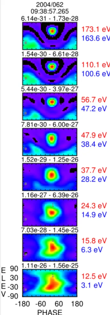
Figure 1 shows an example set of PT plots from a typical foreshock eVDF obtained by the LEEA analyzer on C2 on 2 March 2004. The column of plots shows data from 8 of the 30 energy steps. At this time the analyzer was returning data in the energy range 5.3 to 2531 eV. The energy steps were selected to provide an overall picture of the eVDF. The center
CLUSTERII.CLUSTER-2.3DX1
6.14e-31 - 1.73e-28 09:38:57.265
2004/062
173.1 eV
163.6 eV
l
s
1.54e-30 - 6.61e-28
110.1 eV
100.6 eV
l
s
5.44e-30 - 3.97e-27 56.7 eV
47.2 eV
l
s
7.81e-30 - 6.00e-27 47.9 eV
38.4 eV
l
s
1.52e-29 - 1.25e-26 37.7 eV
28.2 eV
l
s
1.16e-27 - 6.39e-26 24.3 eV
14.9 eV
l
s
7.03e-28 - 1.45e-25 15.8 eV
6.3 eV
l
s
-180 -60 60 180 PHASE -90
-30 30 90 E L E V
1.11e-26 - 1.56e-25 12.5 eV
3.1 eV
l
s
Fig. 1.An example set of PT plots from a typical foreshock eVDF showing the electron core, halo, strahl and return populations. The solid circle and triangle are projections of the magnetic field. Field aligned strahl and return populations (upper 2 plots) are centered on the field projections while the halo and core moving radially outward from the sun are centered in the plot itself. Data is plotted in units of (s3cm−6). Red energy labels are the center energy used for each PT plot while corresponding blue labels are the potential corrected energies.
energy of each plot is given at the right in red. The value in blue below that is the potential corrected center energy. The scaling range used in each autoscaled plot is given above it. These can be used to determine the amount of variation in velocity space density within a shell as well as the fall off in velocity space density over multiple shells.
10 100 1000
1e-06 1e-05 1e-04
10 100 1000
7.0 8.8 10.6 12.4 14.2
100 125 150 175 200
3.6 4.5 5.4 6.3 7.2
0 72 144 216 288
09:00 09:15 09:30 09:45 10:00 10:15
Time (Hr:Min) -90
-54 -18 18 54
2004 062 08:50:00.000
Z 4 5
e V
e V
DEF
Z 6 7
CLUSTERII.CLUSTER1.PEACE / FGM
T e
V
F c e
H z
B n
T
B φ
d e g
B θ
d e g
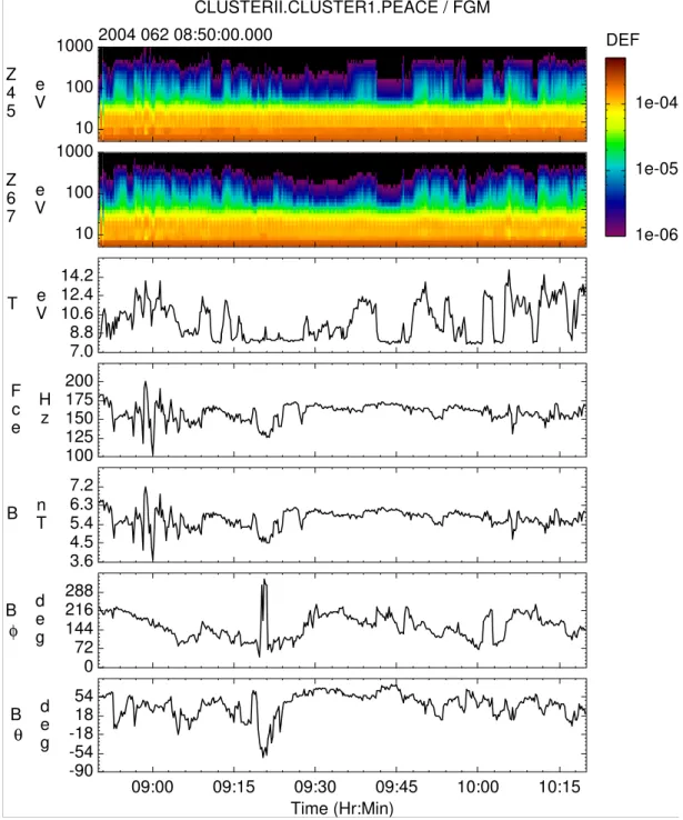
Fig. 2.Spectrograms of the differential energy flux (erg cm−2−sr−s). The data in the top-most plot are from the summed 4–5 polar zones and that in the lower plot are from the summed 6–7 polar zones. Together they cover an elevation from−30◦to 30◦ in the instrument frame of reference. From top to bottom, the other panels show the electron temperature, the electron cyclotron frequency and the spherical components of the magnetic field covering the time frame during which intervals of scattering of the strahl are observed. All data are from C1.
uppermost plot contains two field-aligned populations. The narrow population centered on the circle are strahl electrons moving anti-sunward while the broader population centered on the triangle are return electrons moving back upstream. There is little difference between the top two plots. Over the next two plots, however, the peak in strahl electrons begins
wind core becomes evident indicated by the broadening of the distribution. The broadening is due to the fact that the thermal velocity at these energies much greater than the flow velocity. Some overlap of the core and halo undoubtedly ex-ists but it is virtually impossible to separate the two in this plot format. In the plots, the return electrons weaken with decreasing energy and are completely gone by 24.3 eV.
One final comment concerning the use of PT plots: multi-ple eVDFs are often shown in a single figure using multimulti-ple columns of PT plots. In this layout the potential corrected energy given at the right of each row will indicate only the energy for the last column of plots. Unless the potential is wildly varying over the time frame being shown, this should be a reasonable value for the other columns of plots.
4 Observations
Figure 2 shows both electron and magnetic field data obtained from C1 between 08:50 and 10:20 UT on 2 March 2004 (day 62). During this time interval there were multiple periods of scattering observed in electrons centered on the energy range of the strahl/halo overlap. The upper two panels in the figure show spectrograms of the electron differential energy flux in units of ergs cm−2−s−sr−eV. The data in the upper plot are from the summed 4–5 polar zones and the lower plot from the summed 6–7 polar zones. Together they cover an elevation from−30◦to 30◦in the
in-strument frame of reference. These are followed by plots of the electron temperature in eV, the local electron cyclotron frequency in Hz, and the components of the magnetic field vector in spherical coordinates. The magnetic field angles are both given in GSE coordinates. The average solar wind speed at this time was 675 km s−1.
In the spectrograms, the continuous band of particles be-low about 50 eV is almost exclusively solar wind core and halo electrons, while the more variable signature above that is primarily strahl and return electrons. The strahl and return electrons, which are both field aligned, flow in opposite di-rections and generally appear at separate elevations. The ob-served gaps in the spectrograms above 50 eV are due to theta rotations in the magnetic field that shift the populations into higher or lower elevation analyzers, which are not included in the figure, and/or to transitions between the foreshock and solar wind (return electrons are a foreshock-only feature).
The electron temperature seen in the third panel separates into periods when the temperature is near a baseline value of about 8 eV and times when the temperature is elevated. Ele-vated temperatures occur in the presence of a return electron population, which makes the temperature an extremely good proxy as to whether or not a spacecraft is interior or exte-rior to the foreshock. The dynamic swings seen in the tem-perature plot result from multiple crossings of the foreshock in this time interval. These are the result of variations in
the magnetic topology which changes the connect/disconnect status of the field lines at the spacecraft to the bow shock.
Scattering in the strahl is only observed outside the fore-shock, that is, it occurs in the absence of return electrons. This is shown in Fig. 3, which shows data from four sequen-tial eVDFs acquired from C2. We use data from C2 here (and C4 later), since it was returning information from all 12 el-evation zones which provided better resolution in theta than was possible from either C1 or C3. The scattering, as will be shown later, is observed in all four spacecraft. Each eVDF is characterized by a column of nine PT plots constructed from a contiguous set of returned energy steps between 15.8 and 87.5 eV. As evidenced by the presence of a return electron population (centered on the triangle), the first two eVDFs are acquired within the foreshock, while the last two are acquired outside the foreshock.
Scattering is clearly evident in the PT plots in the last two eVDFs beginning at about 56.7 eV and continuing to lower energies. The picture painted by the PT plots is complex. If we use the solar wind characteristics provided in the second column of plots as a base (and there really is no reason to a priori expect them to be the same as those which led to the scattering), then we see that the scattering begins in energy where the high energy tail of the halo electrons would begin to overlap the strahl. The scattering appears as a tongue of electrons that connects the strahl with a second population of electrons located at the opposite end of the tongue. This sec-ond population of electrons is not the halo, at least not in its classical definition because it is sitting too far off the ecliptic, as can be seen by comparing the expected view of the solar wind from the PT plots of column 2 with those of columns 3 and 4. For descriptive purposes we will refer to this popula-tion of electrons as the proto-halo. Interestingly, there is no halo seen in the 37.7 eV energy PT plots in conjunction with the scattering. It is not clear if the halo has not formed at this energy or has been completely disrupted by the scattering.
There are two additional features that should be noted in Fig. 3 besides the scattering. The first is that the proto-halo is not field-aligned, otherwise it would be centered on the triangle in the plots. This requires a mechanism to keep the population bunched in pitch-angle – perhaps trapping within a wave. We will return to this point later when we look at the local wave field. The second is that at energies beginning near 30.1 eV both the halo and proto-halo can be seen in the PT plots. There is virtually no strahl signature at these ener-gies. At lower energies the proto-halo weakens and the halo strengthens until eventually the proto-halo appears to com-pletely merge with the halo.
CLUSTERII.CLUSTER-2.PEACE.3DX1.CPX1L
2.15e-30 - 1.65e-27
09:41:21.872 2004/062
l
s
3.78e-30 - 3.10e-27
l
s
5.43e-30 - 4.30e-27
l
s
7.15e-30 - 5.67e-27
l
s
1.50e-29 - 1.04e-26
l
s
6.05e-29 - 2.84e-26
l
s
5.87e-28 - 5.74e-26
l
s
1.20e-27 - 1.01e-25
l
s
-180 -60 60 180 PHASE -90
-30 30 90 E L E V
8.04e-27 - 1.34e-25
l
s
2.44e-30 - 1.90e-27
09:41:25.897 2004/062
l
s
3.75e-30 - 2.90e-27
l
s
5.60e-30 - 4.31e-27
l
s
6.16e-30 - 5.22e-27
l
s
2.09e-29 - 1.09e-26
l
s
7.06e-29 - 2.53e-26
l
s
4.96e-28 - 5.70e-26
l
s
1.12e-27 - 9.45e-26
l
s
5.75e-27 - 1.48e-25
l
s
1.98e-30 - 1.36e-27
09:41:29.913 2004/062
l
s
3.61e-30 - 2.43e-27 l
s
5.15e-30 - 3.61e-27 l
s
5.16e-30 - 4.41e-27 l
s
1.69e-29 - 1.13e-26 l
s
3.49e-29 - 2.64e-26 l
s
7.89e-29 - 5.32e-26 l
s
1.36e-27 - 8.37e-26 l
s
5.57e-27 - 1.23e-25 l
s
2.11e-30 - 1.58e-27
09:41:33.931 2004/062
87.5 eV
80.1 eV
l
s
2.86e-30 - 2.28e-27
70.5 eV
63.1 eV
l
s
4.35e-30 - 3.72e-27
56.7 eV
49.4 eV
l
s
4.79e-30 - 4.19e-27
47.9 eV
40.5 eV
l
s
1.81e-29 - 8.57e-27
37.7 eV
30.3 eV
l
s
3.63e-29 - 2.27e-26
30.1 eV
22.7 eV
l
s
3.09e-28 - 4.75e-26
24.3 eV
17.0 eV
l
s
3.18e-27 - 8.78e-26
19.6 eV
12.2 eV
l
s
9.25e-27 - 1.23e-25
15.8 eV
8.4 eV
l
s
Fig. 3. A sets of PT plots from four successive eVDFs across the foreshock boundary. First two eVDFs were taken in the foreshock, as evidenced by the return electron population centered on the triangle. The last two eVDFs show scattering of the strahl beginning about 47.9 eV. The scattering is seen as a tongue of particles extending from the strahl toward the opposite magnetic field projection. The enhanced electron population at the end of the tongue is what we have termed the proto-halo.
– The orientation of the magnetic field lies closer to the ecliptic plane, hence the more horizontal appearance of the scattering.
– The proto-halo appears less intense than seen in Fig. 3.
– The halo extends up to 38.9 eV.
– At 38.9 eV the strahl, halo, and proto-halo all coexist in all three eVDFs shown.
Despite the differences between the figures, the overarching characteristics of the scattering remain unchanged. The scat-tering appears initially as a tongue of electrons that extends
along a line that would connect the two magnetic field projec-tions, there is a formation of a proto-halo electron signature that is not field-aligned, and there is an energy range over which both the halo and proto-halo populations coexist.
CLUSTERII.CLUSTER-4.PEACE.3DX1.CPX1L
1.28e-31 - 1.51e-27
09:22:21.153 2004/062
l s
2.88e-30 - 2.45e-27
l s
6.76e-30 - 3.93e-27
l s
9.88e-30 - 5.39e-27
l
s
1.65e-29 - 8.25e-27
l s
2.63e-28 - 2.17e-26
l
s
1.06e-27 - 4.58e-26
l
s
3.45e-27 - 7.23e-26
l s
-180 -60 60 180
PHASE -90
-30 30 90 E L E V
8.96e-27 - 1.12e-25
l
s
4.24e-31 - 1.46e-27
09:22:25.163 2004/062
l
s
8.88e-31 - 2.48e-27
l
s
6.18e-32 - 3.65e-27
l
s
8.98e-31 - 5.39e-27
l
s
8.92e-30 - 8.34e-27
l
s
8.77e-29 - 2.17e-26
l
s
6.93e-28 - 4.44e-26
l
s
2.82e-27 - 6.90e-26
l
s
1.13e-26 - 1.09e-25
l
s
8.99e-32 - 1.41e-27
09:22:29.172 2004/062
94 eV 84 eV l
s
1.34e-31 - 2.42e-27
75 eV 65 eV l
s
4.08e-30 - 3.69e-27
60 eV 50 eV
l
s
5.39e-30 - 4.60e-27
48 eV 38 eV
l
s
1.15e-29 - 8.04e-27
39 eV 29 eV l
s
5.41e-29 - 2.08e-26
31 eV 21 eV l
s
6.43e-28 - 3.96e-26
25 eV 16 eV l
s
4.77e-27 - 7.74e-26
21 eV 11 eV l
s
6.88e-27 - 1.02e-25
16 eV 7 eV l
s
Fig. 4.PT plots from a set of three successive eVDFs with a more horizontal magnetic field orientation. The proto-halo is less dominant in these plots and the halo appears at a higher in energy than in Fig. 3.
and will be slightly different from the center energies of the analyzers on the other three spacecraft. Also recall that C1 and C3 at this time are returning data with only half the theta resolution as C3 and C4.
Figure 6 shows a long term look at the scattering. The top plot is the electron temperature from C2 over a 12 min time period between 10:00 and 10:12 UT. Transitions between the foreshock and solar wind occur at about 10:01, 10:03, 10:05, 10:10 and 10:11 UT. The bottom set of PT plots spans this interval. (We show only the 37.3 eV energy step from each
CLUSTERII.PEACE
1.11e-31 - 5.31e-28 09:59:57.330
2004/062 C-1
l
s
8.86e-30 - 1.04e-27
l
s
1.35e-29 - 1.69e-27
l
s
4.08e-30 - 3.14e-27
l
s
1.20e-30 - 8.85e-27
l
s
3.22e-29 - 2.48e-26
l
s
2.67e-28 - 4.62e-26
l
s
-180 -60 60 180 PHASE -90 -30 30 90 E L E V
2.36e-27 - 7.82e-26
l
s
9.62e-31 - 8.94e-28 09:59:58.618
2004/062 C-2
l
s
1.76e-31 - 1.67e-27
l
s
2.85e-30 - 2.70e-27
l
s
2.15e-30 - 3.41e-27
l
s
2.58e-30 - 1.04e-26
l
s
2.58e-29 - 2.99e-26
l
s
3.58e-30 - 4.96e-26
l
s
2.14e-27 - 8.13e-26
l
s
6.64e-31 - 5.26e-28 09:59:57.390
2004/062 C-3
l
s
1.24e-30 - 9.48e-28
l
s
2.66e-30 - 1.93e-27
l
s
1.24e-30 - 3.40e-27
l
s
2.12e-29 - 1.11e-26
l
s
7.50e-29 - 2.17e-26
l
s
7.54e-28 - 5.42e-26
l
s
2.16e-27 - 7.35e-26
l
s
2.71e-31 - 7.18e-28 09:59:58.914 2004/062 C-4 93.6 eV 83.6 eV l s
5.56e-31 - 1.45e-27
74.6 eV 64.7 eV l
s
1.72e-30 - 2.13e-27
60.1 eV 50.2 eV l
s
2.92e-30 - 3.35e-27
48.0 eV 38.1 eV l
s
6.64e-30 - 1.06e-26
38.9 eV 29.0 eV l
s
2.80e-30 - 2.50e-26
31.1 eV 21.2 eV l
s
4.50e-28 - 4.40e-26
25.4 eV 15.5 eV l
s
2.32e-27 - 7.50e-26
20.6 eV 10.6 eV l
s
Fig. 5.PT plots of near simultaneous eVDFs as seen on all four spacecraft. There is little difference between the measurements, which are spatially separated by about 230 km.
5 Discussion
There is general agreement that observations of increased pitch-angle broadening in the strahl with distance from the sun is the result of scattering. Simulations suggest that the broadening is due to a mixture of Coulomb collisions and scattering off of either a tenuous background of sunward traveling whistler waves (e.g., Vocks et al., 2005) or off of broadband whistler turbulence (Pierrard et al., 2011). Both produce results that are consistent with the observations of the strahl. It is debatable, however, how applicable the sim-ulation results are to the data presented here. At 1 AU the scattering mechanisms invoked in the simulations of Vocks et al. (2008); Pierrard et al. (2011) and others, are basically weak scattering mechanisms with long mean free paths. And while their effects are easily recognizable when comparing distributions separated by large distances, they are virtually unobservable in individual local eVDFs. Were this not so, scattering signatures in the eVDFs would be ubiquitous in the solar wind.
The scattering observed in the PT plots in Figs. 3 and 4 is both intense and highly energy dependent. In Fig. 3 the scattering occurs within an energy window that extends from 30.1 to 47.9 eV. Active scattering is identified by the exis-tence of a tongue of electrons originating at or near the strahl. Scattered electrons can be, and indeed are, seen at lower en-ergies, but these electrons are assumed to be scattered elec-trons that have been degraded in energy and not elecelec-trons that have a source within the energy window in which they are observed unless there is scattering also occurring in the halo. There is some variation in the location of the energy window with which the active scattering is observed over the entire event, but not by more than an energy channel.
00:00 01:00 02:00 03:00 04:00 05:00 06:00 07:00 08:00 09:00 10:00 11:00 12:00 Time (Min:Sec)
7 9 11 13 15
172004 062 10:00:00.000
CLUSTERII.CLUSTER2.PEACE / FGM
T e V
CLUSTERII.CLUSTER-2.PEACE.3DX1.CPX1L
2004 062 (37.7 eV)
7.70e-30 - 1.16e-26 09:59:58.618
l
s
1.32e-30 - 9.27e-27 10:00:22.718
l
s
4.15e-29 - 9.42e-27 10:00:46.821
l
s
2.49e-29 - 9.62e-27 10:01:10.924
l
s
6.93e-29 - 1.09e-26 10:01:35.025
l
s
1.09e-29 - 1.24e-26 10:01:59.127
l
s
3.17e-29 - 1.19e-26 10:02:23.231
l
s
3.94e-30 - 1.40e-26 10:02:47.331
l
s
7.94e-30 - 7.49e-27 10:03:11.435
l s
7.01e-30 - 8.82e-27 10:03:35.537
l s
5.23e-30 - 9.18e-27 10:03:59.639
l s
4.26e-29 - 6.97e-27 10:04:23.738
l
s
2.02e-29 - 8.48e-27 10:04:47.844
l
s
2.08e-29 - 1.39e-26 10:05:11.944
l
s
1.88e-28 - 1.19e-26 10:05:36.047
l
s
7.93e-29 - 1.70e-26 10:06:00.151
l s
8.09e-29 - 9.99e-27 10:06:24.252
l s
1.41e-29 - 1.21e-26 10:06:48.355
l s
1.64e-29 - 1.08e-26 10:07:12.448
l
s
2.89e-29 - 1.03e-26 10:07:36.559
l
s
1.77e-30 - 1.11e-26 10:08:00.656
l
s
2.51e-30 - 1.15e-26 10:08:24.764
l
s
2.43e-29 - 1.22e-26 10:08:48.865
l
s
1.22e-29 - 1.02e-26 10:09:12.961
l
s
4.66e-31 - 1.12e-26 10:09:37.070
l
s
-180 -30 120 PHASE -90
-3030 90 E L E V
1.87e-30 - 9.51e-27 10:10:01.172
l
s
4.84e-30 - 7.93e-27 10:10:25.275
l
s
4.89e-29 - 8.15e-27 10:10:49.370
l
s
4.78e-29 - 1.21e-26 10:11:13.479
l
s
5.06e-30 - 1.25e-26 10:11:37.581
l
s
Fig. 6.Comparison between eVDFs inside and outside the foreshock showing that scattering is seen only outside the foreshock. Upper plot shows the electron temperature over a 12 min time frame. The spacecraft are in the foreshock during times that the electron temperature is off the baseline value of about 8 eV. The lower plot shows a time series of PT plots at a fixed energy of 37.7 eV. The PT plots are not sequential in time having a 24 s cadence. Scattering is seen to occur only during the times when the temperature is at its baseline value.
Despite these problems, we can however, make a rough es-timate of the scattering strength. In Fig. 3 the two energy channels between 37.7 and 47.9 eV consist basically of strahl and scattered strahl populations. There are very few halo electrons that first appear in significant intensity at 30.1 eV. Using the technique described in Vi˜nas et al. (2010) to
0.10 1.00 10.00 100.00
10:00 10:03 10:06 10:09 10:12
09:57
Time (Hr:Min) 0.10
1.00
7.5 10.0 12.5 15.0 17.5 20.0
1e-10 1e-08 1e-06 1e-04 1e-02 1e+00
2004 062 09:57:00.000
F r e q u e n c y
H z
F r e q u e n c y
H
z T
e V
Power (nT**2/Hz)
C2 /FGM/STAFF Dynamic Power Spectrograms
STAFF
FGM
Fig. 7.Dynamic power spectrograms from STAFF (upper panel) and FGM (lower panel) over a time period that includes the interval shown in Fig. 6. The electron temperature is over-plotted in the lower panel. There is increased wave power in the foreshock especially at the lower frequencies. Puzzling is the lack of any coherent wave signature outside the foreshock where the scattering is observed.
of 0.06 cm−3and an average total density of 0.20 cm−3. This implies that a minimum of 70 % of the strahl has been scat-tered within the selected energy range. The value would be higher if we included the scattered particles that can be seen below the integration energy, but those are more difficult to isolate from the halo.
The scattering efficiency is also dependent on the length over which the scattering occurs. This can’t be directly de-termined but it can be argued that it is probably short. This follows from the highly non-equilibrium features observed in the PT plots including the proto-halo and the tongue of scattered particles. In the absence of the any scattering these should rapidly relax back into an state of equilibrium. Ob-servations of scattering throughout the solar wind portion of the Cluster orbit from which this data was taken suggests a minimum distance over which the scattering is occurring of at least 10RE.
The scattering seen in the data requires the existence of a local intense scattering mechanism which is active within the solar wind but is not present within the foreshock. Such scattering could be provided by magnetic fluctuations and in Fig. 6 we show the local magnetic wave spectra
cover-ing the time period shown in Fig. 7. The figure contains two plots of the magnetic field dynamic power spectra derived from data from C2 between 09:57 and 10:12 UT. The upper plot uses on-board precomputed STAFF spectral data (ob-tained from the CAA) and covers the frequency range 0.1 to 200 Hz. The lower plot, which covers the frequency range 0.02 to 2 Hz, was constructed directly from 5 vectors/s FGM magnetic field data.
The FGM based power density spectra were constructed by first passing the field data through a Savitsky-Golay filter separating it into two frequency bands, one above and one below 0.1 Hz. The power spectra were then computed over each band using the Maximum Entropy Method (MEM). The dynamic power spectra in the low frequency band was con-structed using a 512 point (102.4 s) window advanced 256 points (51.2 s) between calculations. In the high frequency band the window size used was 128 points (25.6 s) and ad-vanced 64 points (12.8 s) between calculations. The power was computed over identical ranges for both bands with the results summed together in a common time grid.
1.23e-31 - 3.27e-28 06:19:58.027
2004/010
139.1 eV 137.2 eV ?
?
3.02e-30 - 5.97e-28
110.1 eV 108.2 eV ?
?
1.40e-29 - 1.11e-27
87.5 eV 85.6 eV ?
?
1.30e-28 - 3.16e-27
70.5 eV 68.6 eV ?
?
6.36e-28 - 8.99e-27
56.7 eV 54.8 eV ?
?
-180 -120 -60 0 60 120 180 PHASE
-90 -60 -30 0 30 60 90
E L E V
2.36e-27 - 2.09e-26
47.9 eV 46.0 eV ?
?
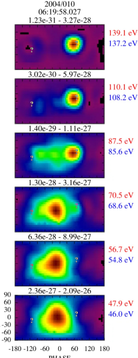
Fig. 8. A set of PT plots from within the time frame identified in Sahraoui et al. (2010) as containing oblique kinetic Alfv´en waves showing intense scattering.
are definite enhancements in the power in the foreshock in the frequencies below 0.06 Hz and to a lesser extent at higher frequencies that are not seen in the solar wind. This is to be expected considering the prevalence of ULF waves in the foreshock (Hoppe et al., 1981; Greenstadt et al., 1995). There is, however, no evidence in these spectra for the presence of monochromatic waves unique to times when scattering is observed. Rather the fluctuations that are present resemble broadband turbulence that might provide guidance as to the source of the scattering. Consequently, these power spec-tra are similar to previous attempts to relate scattering of the strahl to whistler turbulence in that there is no evidence for the existence of such waves. The power essentially disap-pears at the (high) frequencies that might scatter strahl elec-trons. Recent studies of the very high range of the solar wind
turbulence spectrum by Alexandrova et al. (2008); Sahraoui et al. (2009, 2010) do not show any evidence of whistler fluctuations. In fact, the two papers by Sahraoui et al. ar-gue that the spectrum from scales of the ion Larmor radius down to the electron inertial length are dominated by highly oblique kinetic Alfv´enic fluctuations. The highly oblique ki-netic Alfv´en wave, however, cannot act as a cyclotron reso-nance source for scattering strahl electrons. In another pa-per we will examine the role of Landau damping of kinetic Alfv´enic turbulence by the strahl. Here we only mention that for Landau resonance to occur, the kinetic Alfv´enic fluctua-tions must have phase speeds parallel to the local magnetic field that are commensurate with the speed of the lower en-ergy strahl population. It is known from recent work by Shay et al. (2011) that such high phase speeds are possible at least near sites of magnetic reconnection in the magnetotail. Tan-talizing additional evidence that kinetic Alfv´enic turbulence may play a role in the evolution of electron strahl is that sim-ilar scattering is observed within one of the time intervals analyzed by Sahraoui et al. (2010) (10 January 2004, 06:05– 06:55 UT). This is one of the time periods that was populated by oblique kinetic Alfv´en waves. An example set of PT plots centered in the interval is shown in Fig. 8. Scattering dur-ing this time period occurs within a narrower energy window and at much higher energies than seen in the 2 March 2004 event but the salient features are still present. Not shown but consistent with the 2 March observations, there was no scat-tering observed in any adjacent times when the spacecraft were known to be in the foreshock. This would suggest that if it is indeed oblique kinetic Alfv´en waves responsible for the scattering, they are either damped or the conditions are not optimal for their production in the foreshock.
6 Conclusions
PT plots in the interval 08:50 to 10:20 UT on 2 March 2004 clearly show evidence of strong scattering of the strahl. This occurs outside of the foreshock and primarily within the en-ergy range which would nominally contain both the strahl and halo populations (30–50 eV). At least at the upper ener-gies where the scattering is observed there is no evidence of a halo population. Whether the lack of a halo is due to the fact that the halo simply does not extend this high in energy or has been totally disrupted by the scattering is not known. In place of the halo, however, there is, for lack of better ter-minology, a proto-halo population which sits slightly off the magnetic field. At lower energies this population appears to coexist with the halo and to eventually merge or become the halo.
scattering is not at all unique to the the time period analyzed. At other times during the orbit, only data from C4 was avail-able and the eVDFs, although having reduced energy and an-gular resolution, were still sufficient to deduce salient scatter-ing traits. These included: no scatterscatter-ing in the foreshock, the existence of a proto-halo, and a tongue of scattered particles along a general line between the magnetic field projection points. Due to the reduced energy resolution the proto-halo is sometimes not seen. The extended observations indicate that a lower limit to the range over which the scattering is occurring is on the order of 10RE.
While there is no direct evidence for the source of the scat-tering, one possibility that will be investigated in a paper in preparation is whether or not oblique kinetic Alfv´en waves might be able to interact with the field-aligned electron strahl. Future observations of this type of strong scattering coupled with simulations might provide better insight into the source of the scattering.
Acknowledgements. The authors would like to acknowledge the work and role the Cluster Active Archive (CAA) and thank the EFW, WHISPER and FGM teams for providing the data used in this study. We would also like to acknowledge the PEACE team at MSSL who worked on and are constantly improving the instrument calibration. CG would like to acknowledge support from NASA Grant NNX10AC90G.
Topical Editor R. Nakamura thanks two anonymous referees for their help in evaluating this paper.
References
Alexandrova, O., Carbone, V., Veltri, P., and Sorriso-Valvo, L.: Small scale energy cascade of the solar wind turbulence, Astro-phys. J. (Lett.), 674, 1153–1157, doi:10.1086/524056, 2008. Bruno, R. and Carbone, V.: The solar wind as a turbulence
labora-tory, J. Living Rev. Solar Phys., 2, http://www.livingreviews.org/ lrsp-2005-4, 2005.
Dum, C. T., Marsch, E., and Pilipp, W.: Determina-tion of wave growth from measured distribuDetermina-tion func-tions and transport theory, J. Plasma Phys., 23, 91–113, doi:10.1017/S0022377800022170, 1980.
Feldman, W. C., Asbridge, J. R., Bame, S. J., Montgomery, M. D., and Gary, S. P.: Solar wind electrons, J. Geophys. Res., 80, 4181–4196, 1975.
Gary, S. P. and Saito, S.: Broadening of solar wind strahl pitch-angles by the electron/electron instability: Particle-in-cell simulations, Geophys. Res. Lett., 34, L14111, doi:10.1029/2007GL030039, 2007.
Gary, S. P., Saito, S., and Li, H.: Cascade of whistler turbulence: Particle-in-cell simulations, Geophys. Res. Lett., 35, L02104, doi:10.1029/2007GL032327, 2008.
Greenstadt, E. W., Le, G., and Strangeway, R. J.: ULF waves in the foreshock, Adv. Space. Res., 15, 71–84, 1995.
Hammond, C. M., Feldman, W. C., McComas, D. J., and Forsyth, R. J.: Variation of electron-strahl width in the high-speed solar wind: ULYSSES observations, Astron. Astrophys., 316, 350– 354, 1996.
Hoppe, M. M., Russell, C. T., Frank, L. A., Eastman, T. E., and Greenstadt, E. W.: Upstream hydromagnetic waves and their as-sociation with backstreaming ion populations: ISEE 1 and 2 ob-servations, J. Geophys. Res., 86, 4471–4492, 1981.
Johnstone, A. D., Alsop, C., Gurge, S., Carter, P. J., Coates, A. J., Coker, A. J., Fazakerley, A. N., Grande, M., Gowen, R. A., Gur-giolo, C., Hancock, B. K., Narheim, B., Preece, A., Sheather, P. H., Winningham, J. D., and Woodcliffe, R. D.: PEACE: A plasma electron and current experiment, Space Sci. Rev., 79, 351–398, 1997.
Lin, R. P.: Wind observations of suprathermal electrons in the inter-planetary medium, Space Sci. Rev., 86, 61–78, 1998.
Maksimovic, M. V., Zouganelis, I., Chaufray, J. Y., Issautier, K., Scime, E. E., Littleton, J. E., Marsch, E., McComas, D. J., Salem, C., Lin, R. P., and Elliott, H.: Radial evolution of the electron dis-tribution functions in the fast solar wind between 0.3 and 1.5 AU, J. Geophys. Res., 110, A09104, doi:10.1029/2005JA011119, 2005.
Marsch, E.: Kinetic physics of the solar corona and solar wind, J. Living Rev. Solar Phys., 3, http://www.livingreviews.org/ lrsp-2006-1, 2006.
Owens, M. J., Crooker, N. U., and Schwadron, N. A.: Suprathermal electron evolution in a Parker spiral magnetic field, J. Geophys. Res., 113, A11104, doi:10.1029/2008JA013294, 2008.
Pierrard, V., Lazar, M., and Schlickeiser, R.: Evolution of the elec-tric distribution function in whistler wave turbulence of the so-lar wind, Phys. Scripta, 269, 421–438, doi:10.1007/s11207-010-9700-7, 2011.
Pilipp, W. G., Miggenrieder, H., Montgomery, M. D., M¨uhlha¨user, K.-H., Rosenbauer, H., and Schwenn, R.: Unusual electron dis-tribution functions in the solar wind derived from the helios plasma experiment: Double-strahl distributions and distributions with an extremely anisotropic core, J. Geophys. Res., 92, 1093– 1101, 1987a.
Pilipp, W. G., Miggenrieder, H., Montgomery, M. D., M¨uhlha¨user, K.-H., Rosenbauer, H., and Schwenn, R.: Characteristics of elec-tron velocity distribution functions in the solar wind derived from Helios Plasma Experiment, J. Geophys. Res., 92, 1075–1092, 1987b.
Pilipp, W. G., Miggenrieder, H., M¨uhlha¨user, K.-H., Rosenbauer, H., Schwenn, R., and Neubauer, F. M.: Variations of electron ve-locity distribution functions in the solar wind, J. Geophys. Res., 92, 1103–1118, 1987c.
Rosenbauer, H., Miggenrieder, H., Montgomery, M. D., and Schwenn, R.: Preliminary results of the Helios plasma experi-ment, in: Physics of Solar Planetary Environments, edited by: Williams, D. J., p. 319, American Geophysical Union, Washing-ton D.C., USA, 1976.
Rosenbauer, H., Schwenn, R., Marsch, E., Meyer, B., H, M., Mont-gomery, M. D., Muhlhausser, K.-H., Pilipp, W., Voges, W., and Zink, S. M.: A survey on initial results of the Helios plasma ex-periment, J. Geophys., 42, 561–580, 1977.
Sahraoui, F., Goldstein, M. L., Robert, P., and Khotyaintsev, Y. V.: Evidence of a cascade and dissipation of solar wind turbulence at electron scales, Phys. Rev. Lett., 102, 231102, 2009.
Saito, S. and Gary, S. P.: Whistler scattering of suprathermal elec-trons in the solar wind: Particle-in-cell simulations, J. Geophys. Res., 112, A06116, doi:10.1029/2006JA012216, 2007a. Saito, S. and Gary, S. P.: All whistlers are not created
equally: Scattering of strahl electrons in the solar wind via particle-in-cell simulations, Geophys. Res. Lett., 34, L01102, doi:10.1029/2006GL028173, 2007b.
Shay, M. A., Drake, J. F., Eastwood, J. P., and Phan, T. D.: Super-Alfv´en propogaion of substrom reconnection signa-tures and poynting flux, Phys. Rev. Lett., 107, 065001-1, doi:10.1103/PhysRevLett107.065001, 2011.
ˇStver´ak, ˇS., Tr´avn´ıˇceik, P., Marsch, E., Fazakerley, A. N., and Sci-eme, E. E.: Radial evolution of nonthermal electron populations in the low-latitude solar wind: Cluster and Ulysses observations, J. Geophys. Res., 115, A05104, doi:10.1029/2008JA013883, 2009.
Vi˜nas, A. F. and Gurgiolo, C.: Spherical harmonic analysis of par-ticle velocity distribution function: Comparison of moments and anisotropies using Cluster data, J. Geophys. Res., 114, A01105, doi:10.1029/2008JA013633, 2009.
Vi˜nas, A. F., Gurgiolo, C., Nieves-Chinchilla, T., Gary, S. P., and Goldstein, M. L.: Whistler waves driven by anisotropic 3D strahl velocity distributions in the solar wind: Cluster observations, in: AIP Proceedings of Solar Wind 12 Conference, edited by: Mak-simovic, M., Issautier, K., Meyer-Vernet, N., Moncuquet, M., and Pantellini, F., p. 265, American Institute of Physics, New York, NY, USA, 2010.
Vocks, C. and Mann, G.: Generation of suprathermal electrons by resonant wave-particle interaction in the solar corona and wind, Astrophys. J., 593, 1134, 2003.
Vocks, C., Lin, R. P., and Mann, G.: Electron halo and strahl for-mation in the solar wind by resonant interaction with whistler waves, Astrophys. J., 627, 540, 2005.