Abstract— This article proposes a new method to solve non-linear magnetostatic problems applied to the modeling of electromagnetic devices. A reduced scalar potential formulation is presented and solved by a hybrid BEM-NRM. It has been implemented and tested in a software called MaGot. We will show that the computation time of this new method is very low. Thus, it could be easily and efficiently used for the pre-sizing of actuators.
Index Terms— actuators, hybrid method BEM-NRM, magnetostatic,
modeling.
I. INTRODUCTION
Numerical simulations of electromagnetic actuators are an increasing industrial need. In general, the designing time and number of prototypes required to design products are higher during the first step of the whole process. Several methods have been proposed for actuators designing. Two of the most popular methods ones are the Finite Element Method (FEM) [1], [2] and the Reluctance Network Method (NRM) [4], [5].
Based on an equivalent magnetic circuit, NRM is an approach enabling the very quick understood of devices functioning. Computational tools have been developed allowing the automatic assembly of equations [4]. Although easy to use, NRM results can be not so accurate in a first step. Thus, the network can be improved by comparing the results with those from the FEM model and rebuilding a more representative NRM. Once the optimal reluctant model is built, it use is very efficient and quick. Unfortunately, the development of the model can be very extensive, especially in devices with significant leakage flux.
Tools based on FEM provides to the user effective representation of the device. Compared to
NRM, the geometric and physical properties are both precisely and quickly described. On the one hand, the FEM is very general and can solve a wide range of problems; on the other hand, resolution times can be prohibitive for pre-sizing actuators. This question is more meaningful in a context of optimization with a large number of parameters.
A Hybrid Method BEM-NRM for
Magnetostatics Problems
Martins Araujo D. 1,2,*, Coulomb J-L. 2;**, Delinchant B. 2, Chadebec O. 2 1
R&D - Power Technology Strategy - Schneider Electric Industries SAS Grenoble, France 31, rue Pierre Mendès – 38320 Eybens
G2ELAB – Grenoble INP - UJF- UMR CNRS 5269 - Grenoble, France 11, rue des Mathématiques BP 46 - 38402 St Martin d'Hères
That’s why a method combining fast computation time and good accuracy would be very
appropriate to the needs of designers during pre-sizing process. Several others methods have been proposed successfully. In particular, the Boundary Element Method (BEM) [6] is very interesting because the mesh of the whole domain is not needed. Other alternative methods using the FEM and the NRM have been already presented in [3], [7].
This paper proposes a hybrid method combining the BEM, for the surrounding region (the air), and
NRM, for magnetic regions. The inclusion of magnetic sources was made in a particular original way which will be discussed in this paper. The Maxwell tensor method is used for torque and force calculations. The computation time is discussed in the conclusion section of this article. The approach will be compared with FEM and NRM in terms of computation times and accuracy.
II. FORMULATION A. Maxwell's Equations for a Magnetostatic Problem
Let us consider Maxwell's equations for a magnetostatic problem:
j
h
curl
, (1)0
b
div
.
(2)For a non-linear magnetic material, we have:
h
h
c
b
where
(
h
)
. (3)Without any surface currents, we have the following boundary conditions:
0
h
h
n
0
b
b
n
2
1
0
h
h
n
2
1
0
b
b
n
(4)
B. Reduced Scalar Potential Formulation
The domain will be split into several simply connected domains in order to verify the existence of scalar potentials [2], [7].
Let us represent the studied domain.
m
eµ
0
µ
j
r
B
Fig. 1.Representation of a magnetostatic problem
with:
m
: is a magnetic region that doesn’t contain any current, this region may optionally containe
: is a region outside that can accept the presence of electric currents.If there is current within a region, the total field can be decomposed [8], [9]:
red
0
h
h
h
, (5)where the field
h
0 is the field created by electric current, i.e. the inductor field. The reduced fieldred
h
derives from a reduced potential. From (2) and (3), we get in each region:m
div
h
c
grad
m
0
(6)
e
div
h
0
grad
e
0
From conservation of the tangential component of
h
, it is possible to find a law that allow to take into account the magnetic sources. Let us define
me the boundary between the domains
e and
mand
t
is the tangent vector to this boundary:m
e
t
me
Fig. 2. Interface between regions and tangent vector.
With (4) and (5), we get :
h
c
grad
m
t
h
0
grad
e
t
(7)By integrating the equation above a path
ab
that belongs to the boundary
me[10], [11], we get:
ab
c 0 e b e a m b m a
ds
t
h
h
(8)This equation expresses the influence of source terms on the potential.
III. BOUNDARY ELEMENT METHOD
A. Fundamental Solution and Poles of the Function
The equation (9) represents the integral equation deduced from the identity of Green. Where
x
0,
y
0represent the pole of the function:
dln G n G y
, x y , x h
e
C 0 0 0
0
(9)
The coefficient
h
x
0,
y
0
varies in function of pole’s position. There are three possibilities: in the
x
0,
y
0
1
,
if
x
0,
y
0
eh
(10)
0 0
,
if
x
0,
y
0
C
e2
1
y
,
x
h
x
0,
y
0
0
,
if
x
0,
y
0
eh
Equation (11) shows the Green’s function used in (9). This function represents an analytical solution of Laplace’s equation in a two-dimensional case:
2
0 2
0
y
y
x
x
ln
2
1
G
x
,
y
,
x
,
y
x
0,
y
0
(11)B. Discretization of
C
e and Matrix SystemThe boundary
C
e of the domain
e is discretized with boundary elements.e
e
C
j
0
i
C
i i
q
u
,
Fig. 3. Boundary discretisation.
N1 i
i
e
C
C
(12)For each element, we have two determine: the potential
and the magnetic flux flowing through the element. To discriminate exact solution and numerical approximation, we will use thefollowing notation:
x
,
y
u
i andC
i.
q
in
y
,
x
for element “i”. Quantities are constantsby element and we use a collocation approach, i.e. the writing of (9) at each element centroid. By discretizing the equation (10), we get:
N1
j C
i j C
i j i
i
dl
q
G
dl
n
G
u
u
h
j j
(13)
This equation can be represented by the following matrix system:
0
Q
T
U
H
BEM
BEM
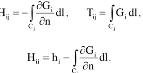
(14)dl n G H
j
C i
ij
T G dl
j
C i
ij
(15) dl
n G h
H
j
C i i
ii
T is an invertible matrix, we can write a relation linking the flux to the potential on the boundary:
BEM BEM
BEM
P
U
Q
(16)
T
H
inv
P
BEM
(17)The matrix represented by equation (17) is a fully populated matrix.
IV. RELUCTANCE NETWORK METHOD (NRM) AND COUPLING BOTH METHODS A. Generalities
In order to take into account the physical behavior of materials and to develop a simple method without decreasing the accuracy of the results, we decompose the magnetic domain into bricks and we introduce a reluctance network inside each of them. This network can optionally contain sources of magnetomotive force. An originality of our approach is that bricks can be subdivised in order to obtain (if needed) a more accurate representation of the magnetic behavior.
10
u
0
k
u
1 1, k
k q
u
kt
ktq
u , kt P kt F
Fig. 4. Introducing NRM in the two bricks of the magnetic domain.
B. Development
Let us suppose a region
m, discretized and composed of M bricks. Each brick kcontain T flux tubes connecting the central potential to the potentials of facets.q
kt is the flow through the facet tof the brickk
, so the following relation can be written [12]:
kt k0 kt
ktkt
u
u
F
P
q
(18)The permeance of a tube can be calculated from its permeability
kt, its lengthL
kt and its cross sectionS
kt [4]:kt kt 0 kt kt
L S
P (19)
C. Potentials elimination
T 1 t kt kt 0 k kt T 1 tkt u u F P
q (20)
T 1 t kt T 1 t kt kt kt 0 kP
P
F
u
u
we get:
kt T 1 t kt T 1 t kt kt kt T 1 t kt T 1 t kt kt kt ktP
P
P
F
F
P
P
u
u
q
(21)
D. Flux elimination
Let us consider a facet shared by two flux tubes. The incoming flux comes in from a single tube, and comes out though the other one. This conservation of the flow can also be expressed by ensuring that the sum flux is equal to zero.
For each facet kt:
t 1 k T 1 t t 1 k T 1 t t 1 k t 1 k t 1 k T 1 t t 1 k T 1 t t 1 k t 1 k t 1 k ktP
P
P
F
F
P
P
u
u
q
(22)
t 2 k T 1 t t 2 k T 1 t t 2 k t 2 k t 2 k T 1 t t 2 k T 1 t t 2 k t 2 k t 2 k ktP
P
P
F
F
P
P
u
u
q
(23)
The sum of both equations links potentials of two adjacent bricks. As the number of facets on equation are the same. It is also applicable on a facet shared by a brick and by an element treated with the boundary element method.
E. Calculation of magnetomotive force
According to Ampere's law and equation (8) and also assuming a uniform field into a subset of the domain bricks, we can deduce the magnetomotive force of a tube with:
kt 0 k c 0kt
h
h
t
ds
F
(24)where ds represents the section of a flux tube. The field
h
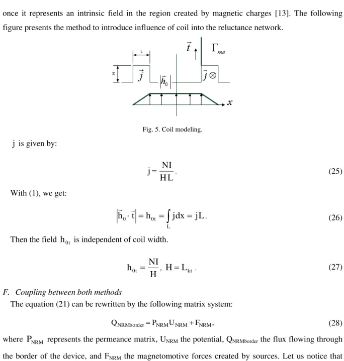
c represents the contribution of theonce it represents an intrinsic field in the region created by magnetic charges [13]. The following figure presents the method to introduce influence of coil into the reluctance network.
Fig. 5. Coil modeling.
j
is given by:L H
NI
j (25)
With (1), we get:
L
j
dx
j
h
t
h
L t 0
0
(26)
Then the field
h
0t is independent of coil width.H
NI
h
0t
H
L
kt (27)F. Coupling between both methods
The equation (21) can be rewritten by the following matrix system:
NRM NRM NRM
NRMborder P U F
Q (28)
where
P
NRM represents the permeance matrix, UNRM the potential, QNRMborder the flux flowing throughthe border of the device, and FNRM the magnetomotive forces created by sources. Let us notice that
NRM
P
is a sparse matrix and have more unknowns than equation.Thanks to (21) and (16), we can easily eliminate external flux unknowns and build a matrix representing the BEM-NRM coupling:
NRM NRM NRM
BEM U F
P (29)
where
P
BEMNRM is build usingP
BEM andP
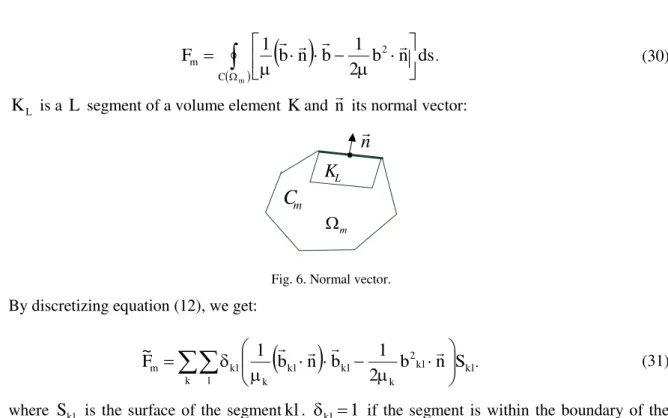
NRM matrix.V. CALCULATING FORCES
ds
n
b
2
1
b
n
b
1
F
m
C
2
m
(30)L
K
is a L segment of a volume element Kand n its normal vector:m
m
C
n
L
K
Fig. 6. Normal vector.
By discretizing equation (12), we get:
klk l
kl 2
k kl kl
k kl
m
b
n
S
2
1
b
n
b
1
F
~
(31)where
S
kl is the surface of the segmentkl
.
kl
1
if the segment is within the boundary of the magnetic region.VI. RESULTS FEM AND BEM-NRM
In this section, we present the comparisons between the FEM model and the BEM-NRM model of the actuator represented by figure 7. The purpose of this section is to validate the proposed method. All the results were obtained in static two-dimension case. The idea is to have a sufficiently large number of static results in order to introduce them into a tool where the study the dynamic behavior of the actuator is possible. However, the dynamic simulation is outside the scope of this work.
µiron
µ0 ATcoil
µmagnet
⃗
Brmagnet
x1
x2
y1
y2
y3
y4
a1
x3
Fig. 7. An U actuator.
We have the following geometrical characteristics:
mm
The magnet is represented by the following physical properties:
B
r
1
T
;µ
r
1
.We use the fixed point method to solve the nonlinear system. The nonlinear ferromagnetic material is represented by an initial permeability and a saturation level in equation 13:
1000
µ
r
;J
s
2
T
,
s 0 r s
0
J
2
H
µ
)
1
µ
(
arctg
J
2
H
µ
B(H)
(32)
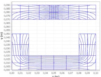
The figure 8 shows the mesh and the field lines of the model BEM-NRM1.
In order to present the comparisons, we have to consider the variation of the air gap
y
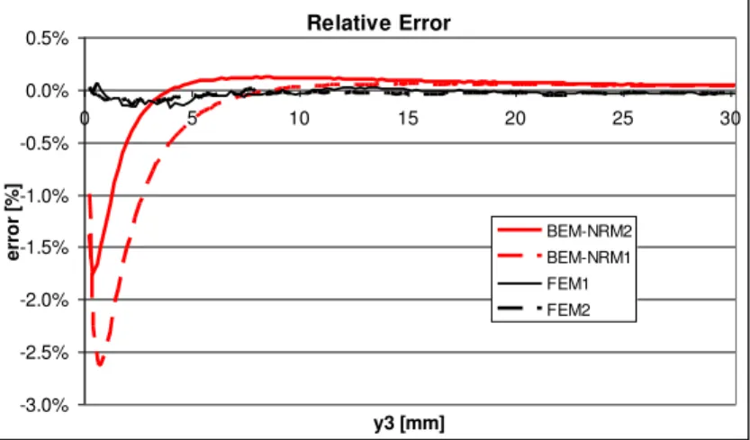
3. The figures 9 and 10 present the force as a function of the errors computed with MaGot (BEM-NRM) and Flux (FEM tool). BEM-NRM2 was obtained by subdivising each brick of BEM-NRM1 in four bricks. In figure 10, FEM1 and FEM2 represent FEM solutions using different mesh size. The idea is to study the evolution of the accuracy and the computation time. The reference solution is obtained by FEMwith a very dense mesh. The error is divided by a reference value of force or torque in order to get a relative one.
Fig. 8. Mesh and field lines of the model BEM-NRM1.
Force
1 10 100 1000
0 5 10 15 20 25 30
y3 [mm]
fo
rc
e
[
N
]
FEM BEM-NRM1 BEM-NRM2
Relative Error
-3.0% -2.5% -2.0% -1.5% -1.0% -0.5% 0.0% 0.5%
0 5 10 15 20 25 30
y3 [mm]
e
rr
o
r
[%
]
BEM-NRM2 BEM-NRM1 FEM1 FEM2
Fig. 10. Relative error in the force.
In a similar way, the calculation of the torque has been studied. It shows the advantages of this approach compared to a pure NRM. In fact, the pure NRM model for rotational motion requires many efforts to be built by designers (due to the leakage fluxes). The figures 11 and 12 show the shape of the torque as a function of the errors.
Torque
0 1 10 100
0 5 10 15 20 25 30
a1 [°]
to
rq
u
e
[
N
.m
]
FEM BEM-NRM1 BEM-NRM2
Fig. 11. Torque developed by the actuator.
Relative Error
-3.5% -3.0% -2.5% -2.0% -1.5% -1.0% -0.5% 0.0% 0.5%
0 5 10 15 20 25 30
a1 [°]
e
rr
o
r
[%
]
FEM1 FEM2 BEM-NRM2 BEM-NRM1
Fig. 12. Relative error in the torque.
TABLE I. FORCE AND TORQUE COMPUTATION TIME
METHOD NUMBER OF ELEMENTS COMPUTATION TIME
FORCE TORQUE FORCE TORQUE
FEM1 1292 6670 03mn02s 05mn52s FEM2 1518 6794 03mn22s 06mn07s
BEM-NRM1 48 48 08s 08s
BEM-NRM2 192 192 02mn16s 02mn09s
We observe that a very low number of elements and a very low computation time (BEM-NRM1) to get an accurate result.
VII. EVALUATION OF A METHOD’S ROBUSTNESS
The purpose of this section is to evaluate the method’s robustness. For the actuator from the previous section, we built four models using the program RelucTool [4], [5] based on NRM. Depending on the time taken for the design of these models, its accuracy is higher or lower. This fact can be highlighted looking at the design process.
Fig. 13. Model NRM1. Fig. 14. Model NRM2. Fig. 15. Model NRM3.
Fig. 16. Model NRM4.
For the results presented below we set the parameters observing the results obtained with the FEM, and then adjusting these parameters. A FEM model built using Flux is show in figure 17.
Fig. 17. FEM Model.
The model NRM2 is closer to the reference (FEM) than the model NRM1 because of the increase of the reluctance airgap11 and airgap12. The NRM2 model represents better the leakages flux. Leakages fluxes around the magnet are also important and this is why the model NRM3 was built.
Despite the positive evolution of these results, they are not enough satisfying. Then a new model
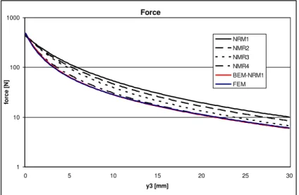
(NRM4) is constructed by studying the actuator in more detailed and, therefore, by again spending more time of development. According to figure 18 and 19, we get good results with this last model
(NRM4). In comparison with this complex procedure, the development of our NRM-BEM approach is very simple and still more accurate.
Force
1 10 100 1000
0 5 10 15 20 25 30
y3 [mm]
fo
rc
e
[
N
]
NRM1 NMR2 NMR3 NMR4 BEM-NRM1 FEM
Relative Error
-15% -10% -5% 0% 5% 10% 15% 20%
0 5 10 15 20 25 30
y3 [mm]
e
rr
e
u
r
[%
]
NRM1 NMR2 NMR3 NMR4 BEM-NRM1
Fig. 19. Relative error in the force.
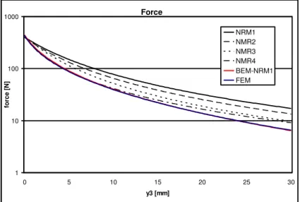
During the process of designing, we are often faced with the need to optimize the structures. This means that the models must be robust to parametric variations. So, we changed two parameters of our actuator: x160mm; x315. The objective here is to evaluate the robustness of the models.
Force
1 10 100 1000
0 5 10 15 20 25 30
y3 [mm]
fo
rc
e
[
N
]
NRM1 NMR2 NMR3 NMR4 BEM-NRM1 FEM
Fig. 20. Magnetic force developed by the actuator changing parameters x1 and x3.
Relative Erreur
-10% -5% 0% 5% 10% 15% 20%
0 5 10 15 20 25 30
y3 [mm]
e
rr
e
u
r
[%
]
BEM-NRM1 NRM1 NMR2 NMR3 NMR4
Fig. 21. Relative error in the force.
significantly decrease the accuracy of the NRM models. However, the BEM-NRM results remain accurate. We can conclude on the good robustness of our new approach.
VIII. CONCLUSION
A hybrid BEM-NRM is has been developed and adapted to the actuators pre-sizing. Magnetic sources are taken into account in a very simple way. The goal of this paper is to present first results of this original approach. The results presented here demonstrate that our method provides very fast and quite accurate computations compared to FEM. It is very important for optimization tasks which are currently very expensive in terms of computation time.
The comparisons between the BEM-NRM and NRM show several advantages of the method we propose. Although obtained results are not practically instantaneous as in the case of NRM, the computational effort is very small. The modeling of the device is more efficient because user does not need to worry about leakages flux. As showed in figure 21, BEM-NRM is more robust than NRM in terms of geometric variations.
The process of pre-sizing electric actuators asks for a fast, accurate and robust method. In this process, we do not have time for long but accurate calculations as FEM. As discussed in Section VII, the construction of a NRM model is long and can requires a specific expertise. Additionally, the FEM
is often used to study the behavior of leakage flux before the construction of the model NRM. So we need to combine both methods and two computational tools which can become long. The proposed method is a good compromise between all requirements.
REFERENCES
[1] J.-L. Coulomb, “Analyse tridimensionnelle des champs électriques et magnétiques par la méthode des éléments finis,” Thèse, INP de Grenoble, 1981.
[2] G. Meunier, “Modèles et formulations en électromagnétisme,” Paris: Hermes Science Publications, 2002.
[3] A. Demenko and J. K. Sykulski, “Network equivalents of nodal and edge elements in electromagnetics,” IEEE Trans. Magn., vol. 38, no. 2, pp. 1305–1308, 2002.
[4] B. du Peloux, L. Gerbaud, F. Wurtz, V. Leconte, and F. Dorschner, “Automatic generation of sizing static models based
on reluctance networks for the optimization of electromagnetic devices,” IEEE Trans. Magn., vol. 42, no. 4, pp. 715–
718, 2006.
[5] B. du Peloux., L. Gerbaud, F. Wurtz, E. Morin "A method and a tool for fast transient simulation of electromechanical devices: application to linear actuators", MOMAG 2010, Brazil (2010)
[6] L. Krahenbuhl, “La méthode des équations intégrales de frontière pour la résolution des problèmes de potentiel en
électrotechnique, et sa formulation axisymétrique,” Ecole Centrale de Lyon, 1983.
[7] A. Demenko, L. Nowak, and W. Szelag, “Reluctance network formed by means of edge element method,” IEEE Trans. Magn., vol. 34, no. 5, pp. 2485–2488, 1998.
[8] P. Dular, “Modélisation du champ magnétique et des courants induits des systèmes tridimensionnels non linéaires,” Univer. de Liège, 1994.
[9] Viet Phuong Bui, Y. Le Floch, G. Meunier, and J.-L. Coulomb, “A New Three-Dimensional (3-D) Scalar Finite
Element Method to Compute To,” IEEE Trans. Magn., vol. 42, no. 4, pp. 1035–1038, 2006.
[10]Y. Choua, “Application de la méthode des éléments finis pour la modélisation de configurations de contrôle non
destructif par courants de Foucault,” Université Paris-Sud 11, 2009.
[11]J. Simkin and C. W. Trowbridge, “Three-dimensional nonlinear electromagnetic field computations, using scalar
potentials,” Electric Power Applications, vol. 127, no. 6, pp. 368–374, 1980.
[12]A. Demenko and K. Hameyer, “Field and field-circuit description of electrical machines,” presented at the Power Electronics and Motion Control Conference. EPE-PEMC. 13th, 2008, pp. 2412–2419.
[13]Shaoming Zheng and Renhong Wang, “A new method for the solution of three dimensional magnetostatic fields, using