Braz. J. Phys. vol.35 número4B

(1)

1106 Brazilian Journal of Physics, vol. 35, no. 4B, December, 2005

Notes on the Quantization of FRW Model in the Presence of a Cosmological

Constant and Radiation

G. A. Monerat, E. V. Corrêa Silva, G. Oliveira-Neto, Departamento de Matemática e Computação, Faculdade de Tecnologia,

Universidade do Estado do Rio de Janeiro, Estrada Resende-Riachuelo, s/no, Morada da Colina

CEP 27523-000, Resende-RJ, Brazil.

L. G. Ferreira Filho,

Departamento de Mecˆanica e Energia, Faculdade de Tecnologia, Universidade do Estado do Rio de Janeiro,

Estrada Resende-Riachuelo, s/no_{, Morada da Colina}

CEP 27523-000, Resende-RJ, Brazil.

and N. A. Lemos

Instituto de F´ısica, Universidade Federal Fluminense, R. Gal. Milton Tavares de Souza s/no_{, Boa Viagem}

CEP 24210-340, Niter´oi-RJ, Brazil (Received on 7 October, 2005)

In the present work, we use the formalism of quantum general relativity in order to quantize a Friedmann-Robertson-Walker model in the presence of a negative cosmological constant and radiation. The model has spatial sections with positive constant curvature. The wave-function of the model satisfies a Wheeler-DeWitt equation, for the scale factor, which has the form of the Schr ¨odinger’s equation for the quartic anharmonic oscillator. We find the eigenvalues and eigenfunctions by using a method first developed by Chhajlany and Mal-nev. After that, we use the eigenfunctions in order to construct wave-packets for evaluating the time-dependent, expected value of the scale factor. We find that, the expected value of the scale factor oscillates between maxi-mum and minimaxi-mum values. Since the scale factor never vanishes, we conclude that the model does not have a singularity.

One of the motivations for the quantization of cosmolog-ical models was that of avoiding the initialBig Bang singu-larity. Since the pioneering work in quantum cosmology due to DeWitt [1], workers in this field have been attempting to prove that quantum cosmological models entail only regular space-times. An important contribution to this issue was given by Hartle and Hawking [2], who proposed the no-boundary boundary condition, which selects only regular space-times to contribute to the wave-function of the Universe, derived in the path integral formalism. Therefore, by construction, theno-boundarywave-functions are everywhere regular and predict a non-singular initial state for the Universe. Using that boundary condition, in certain particular cases the no-boundary wave-function can be explicitly computed [2–4]. Another way by which one may compute the wave-function of the Universe is by directly solving the Wheeler-DeWitt equa-tion [1]. The wave-funcequa-tion of the Universe for some impor-tant models have been computed using this approach [5–10].

Several important theoretical results and predictions in quantum cosmology have been obtained with a negative cos-mological constant [11], [12] and [3]. Besides that, we think it is important to understand more about such models which rep-resent bound Universes (analogous to uni-dimensional atoms, in the present situation).

In the present paper, we use the formalism of quantum cos-mology in order to quantize a Friedmann-Robertson-Walker model in the presence of a negative cosmological constant and radiation. The radiation is treated by means of the

vari-ational formalism developed by Schutz [13]. The model has spatial sections with positive constant curvature. The wave-function of the model satisfies a Wheeler-DeWitt equation, for the scale factor, which has the form of the Schr¨odinger’s equation for the quartic anharmonic oscillator. We find the eigenvalues and eigenfunctions by using a method first devel-oped by Chhajlany and Malnev. After that, we use the eigen-functions in order to construct wave-packets for evaluating the time-dependent, expected value of the scale factor. We find that the expectation value of the scale factor shows bounded oscillations and since it never vanishes, we conclude that the model does not have a singularity.

Friedmann-Robertson-Walker cosmological models are characterized by the scale factora(t)and have the following line element,

ds2=−N(t)2_dt2₊_a₍_t₎2 µ

dr2 1−kr2+r

2_d_Ω2 ¶

, (1)

(2)

G. A. Monerat et. al. 1107

Tµ,ν= (ρ+p)UµUν−pgµ,ν−Λgµ,ν, (2)

whereρandpare the energy density and pressure of the fluid, respectively. Here, we assume that p=ρ/3, which is the equation of state for radiation. This choice may be consid-ered as a first approximation to treat the initial content of the Universe and it was made as a matter of simplicity. It is clear that a more complete treatment should describe the radiation, present in the primordial Universe, in terms of the electro-magnetic field. Einstein’s equations for the metric (1) and the energy momentum tensor (2) are equivalent to the Hamilton equations generated by the super-hamiltonian constraint

H

₌₋p

2

a

12−3a

2_+Λ_a4₊_p

T, (3)

wherepaandpT are the momenta canonically conjugated to

a andT the latter being the canonical variable associated to the fluid [10].

In the case of the model studied here, the scale factor per-forms bounded oscillations. When the scale factor vanishes we have the formation of a singularity which may be either a Big Bangor aBig Crunch.

Using the Dirac formalism for quantizing constrained sys-tems [14], we obtain from

H

_{Eq. (3) the following}

Wheeler-DeWitt equation,

µ 1 12

∂2

∂a2−3a 2₊_Λ_a4

¶

Ψ(a,τ) =−i ∂

∂τΨ(a,τ), (4)

whereΨ(a,τ)is the wave-function of the model and the new variableτ=−T has been introduced.

The operator ˆ

H

_{is self-adjoint [8] with respect to the}

inter-nal product,

(Ψ,Φ) = Z ∞

0

daΨ(a,τ)∗Φ(a,τ), (5) if the wave functions are restricted to the set of those satisfying eitherΨ(0,τ) =0 orΨ′(0,τ) =0, where the prime′means the partial derivative with respect toa.

The Wheeler-DeWitt equation (4) is the Schr¨odinger equa-tion for the quartic anharmonic oscillator and may be solved by writingΨ(a,τ)as

Ψ(a,τ) =e−iEτη(a) (6)

whereη(a)depends solely ona. Thenη(a)satisfies the eigen-value equation

−d

2η(_a₎

da2 +Ve(a)η(a) =12Eη(a), (7) where the effective potentialVe(a)is given by

Ve(a) =36a2−12Λa4. (8)

The method of Chhajlany and Malnev [15] starts with the addition of an extra term to the original anharmonic oscillator potential, so that the modified Hamiltonian admits a subset of manifestly normalizable solutions. In the case we are consid-ering, the extra term to be added to the effective potential (8) is proportional toa6. In terms of that new enlarged potential, the eigenvalue equation (7) may be re-written as

η′′₍

a) + (ε−αa2−ba4−ca6)η(a) = 0 (9) whereε=12E, α=36,b=−12Λ,cis a parameter to be determined by the method. TheAnsatzfor the solution of Eq. (9) takes the form

η(a) =Nexp³−c

4a 4₋γ

2a 2´

v(a), (10) and has finite norm forc>0. Here,v(a)is a polynomial of a certain degree, yet to be chosen; the parameterγ is to be chosen according to our convenience, as we shall see;Nis a normalization factor. The method is based on the fact, shown in Ref. [15], that the larger the degree of the polynomialv(a), the smallercis. Therefore, if one increases the order ofv(a), the energy eigenvalues predicted by the present method tend monotonically, from above, to the energy eigenvalues of the original problem. One important property of the method is that the convergence is very fast. This means that one does not need to use a polynomial of very large order to obtain a good agreement with the energies of anharmonic oscillators already computed in the literature by other methods.

The next step is the substitution of theAnsatz(10) into the differential equation (9), which gives rise to an equation for the polynomialv(a). Then, writingv(a) =∑nβnanand

insert-ing it in that equation for the polynomialv(a), along with the condition 2cγ=b[15], we manage to find:

(ε−γ)β0+2β2=0, (ε−3γ)β1+6β3=0, (11) and the general recurrence relation for the polynomial coeffi-cientsβn,

(n+4)(n+3)βn+4 + [ε−γ(2n+5)]βn+2

+[γ2₋_α₋

c(2n+3)]βn = 0 (12)

forn≥0. The degree of the polynomialv(a)is fixed to be, sayK, by imposing the following conditions in (12),

βK6=0, βK+2=βK+4=0. (13) Due to the nature of the recurrence relation (12), it is clear that by fixingK to be even (odd) the resulting polynomial v(a)

will be even (odd). Then, the coefficientsβn, n=2,4, ...,K

(3)

1108 Brazilian Journal of Physics, vol. 35, no. 4B, December, 2005

Eqs. (12) and (13) require that the coefficientβK must

van-ish; then

γ2₌_α₊_c₍₂_K₊₃₎_. ₍₁₄₎

Combining this with 2cγ=b, we obtain a cubic algebraic equation in the parameterc,

4c3(2K+3) +4αc2−b2=0. (15) The solutions of this equation depend on the known parame-tersbandK. We must find the real, positive root to this equa-tion so that theAnsatzEq. (10) be normalizable. That real positive root, as proved in Ref. [15], is a monotonically de-creasing function ofK. Therefore, the greater the polynomial degree, the better the agreement between the energy eigenval-ues obtained by this method and the actual energy eigenvaleigenval-ues. Now, by setting the condition βK+2=0 in Eq. (12) we may determine the corresponding (m+1) energy eigenval-uesεand polynomial coefficientsβn. With those coefficients

βn, we obtain the appropriate polynomial vl(a); the index

l=1,2, ...,m+1 represents the energy level, for each of which we shall have an eigenfunction ηl(a) and a wave-function

Ψl(a,τ) =exp(−iElτ)ηl(a), according to Eqs. (6) and (10).

We construct a general solution to the Wheeler-DeWitt equation (4) by taking linear combinations of theΨl(a,τ)’s,

Θ(a,τ) =

m+1

∑

l=1

Al(E)ηl(a)e−iElτ, (16)

as a matter of simplicity we shall set the coefficientsAl(E)to

one, in what follows.

With those combinations we compute the expected value for the scale factora, following themany worlds interpreta-tionof quantum mechanics [16]. In the present situation, we may write the expected value for the scale factorais

hai(τ) =

R∞

0 a|Θ(a,τ)|2da R∞

0 |Θ(a,τ)|2da

. (17)

In order to obtain the results, we shall use the value of

Λ=−0.1, therefore one hasb=1.2 in Eq. (9). Also, we shall fix the polynomial degree to beK=45. It means that, we shall have 23 energy levels and 23 eigenfunctionsηl(a).

Using the values of K and b, we solved Eq. (15) to find c=0.090068960669615962974. Now, we obtain the energy levels; they are listed in Table I. The first few lowest energy levels are in agreement with the ones computed, perturba-tively, by Landau for the quartic anharmonic potential, equiv-alent to the present case [17]. For the present case, we may also compare the original potential Eq. (8) with the auxiliary potential,

U(a) =36a2+1.2a4+0.008112417676a6. (18) Then, we obtain a relative errorεof less than 1% in the inter-vala∈[0,2.728021504]. Whereεis given by,

ε=

¯ ¯ ¯ ¯

V(a)−U(a) V(a)

¯ ¯ ¯ ¯

. (19)

After that, we substitute the energies in the set of Eqs. (12) and compute the coefficientsβn. With theseβn, we write the

followingη(a,τ), according to Eq. (10),

ηl(a) =Nlvl(a)×

e−0.022517240167403990744a4−3.3307811899866029985a2, (20) where

vl(a) =

22

∑

i=0

Al,2i+1a2i+1. (21)

The coefficients Nl are normalization coefficients and i =

0,1, ...,m. The complete list of values for the Nl’s and the

Al,2i+1’s as well as the study of the cases wherek=0 and k=−1 are given in reference [18].

Next, we construct the wave-packetΘ(a,τ)with the aid of theηl(a), according to Eqs. (16), (20) and the energy levels

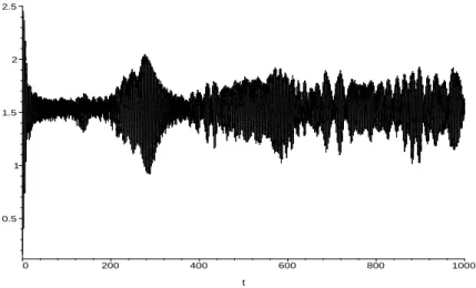
in Table I. Finally, using the wave-packetΘ(a,τ)we compute the expected value for the scale factora, Eq. (17). The result is shown in Fig. 1; it can be seen thathaidoes not vanish, therefore we may say that the quantization of this model re-moved the singularities it had at the classical level. It is clear from Fig. 1, also, thathaiperforms bounded oscillations. That means that the spatial sectionsS3’s oscillate between finite maximum and minimum radius.

Level k=1

E1 1.5103016760578712464 E2 3.5509871014722954423 E3 5.6230931685080087038 E4 7.7256531719671366439 E5 9.8577817762723638293 E6 12.018664367453930157 E7 14.207548216681935132 E8 16.423735430300010131 E9 18.666574187417793427 E10 20.935469528987599984 E11 23.229800589269486517 E12 25.549220854858484858 E13 27.892697492531834013 E14 30.260978882469751228 E15 32.651319599290796010 E16 35.066840708164574204 E17 37.502643477205645295 E18 39.963027226267456788 E19 42.443644402959303694 E20 44.946892054208187300 E21 47.470929938318337116 E22 50.01608754545613080 E23 52.581852999800707709

TABLE I:The lowest calculated energy levels.

Acknowledgments

(4)

G. A. Monerat et. al. 1109

0.5 1 1.5 2 2.5

0 200 400 600 800 1000

t

FIG. 1:Behavior of the expectation value of the scalar factor.

[1] B. S. DeWitt, Phys. Rev. D160, 1113 (1967).

[2] J. B. Hartle and S. W. Hawking, Phys. Rev.D28, 2960 (1983). [3] G. Oliveira-Neto, Phys. Rev. D58, 10750 (1998);

[4] Y. Fujiwara et al., Class. Quantum Grav.7163 (1992); Phys. Rev. D44, 1756 (1991); J. Louko and P. J. Ruback, Class. Quantum Grav.8, 91 (1991); J. J. Halliwell and J. Louko, Phys. Rev. D 4

¯2, 3997 (1990);

[5] Mariam Bouhmadi-Lopez and Paulo Vargas Moniz, Phys. Rev. D71, 063521 (2005); I. G. Moss and W. A. Wright, Phys. Rev. D29, 1067 (1984); M. J. Gotay and J. Demaret, Phys. Rev. D 28, 2402 (1983);

[6] O. Bertolami and J. M. Mour˜ao, Class. Quantum Grav.8, 1271 (1991).

[7] M. Cavaglia, V. Alfaro and A. T. Filippov, Int. J. Mod. Phys. A 10, 611 (1995).

[8] N. A. Lemos, J. Math. Phys.37, 1449 (1996);

[9] N. A. Lemos, G. A. Monerat, Gen. Rel. Grav.35, 423 (2003); J. Acacio de Barros and N. Pinto-Neto, Int. J. Mod. Phys. D 7, 201 (1998); J. Acacio de Barros, N. Pinto-Neto and M. A. Sagioro-Leal, Phys. Lett. A241, 229 (1998).

[10] F. G. Alvarenga, J. C. Fabris, N. A. Lemos, G. A. Monerat, Gen. Rel. Grav.34, 651 (2002).

[11] S. Carlip, Phys. Rev. Lett.794071 (1997).

[12] M. Anderson, S. Carlip, J.G. Ratcliffe, S. Surya and S.T. Tschantz, Class. Quant. Grav.21729, (2004).

[13] Schutz, B. F., Phys. Rev. D2, 2762, (1970); Schutz, B. F., Phys. Rev. D4, 3359, (1971).

[14] P. A. M. Dirac, Can. J. Math.2, 129 (1950); Proc. Roy. Soc. London A bf 249, 326 and 333 (1958); Phys. Rev.114, 924 (1959).

[15] S. C. Chhajlany and V. N. Malnev, Phys. Rev. A, vol 42, No. 5, 3111 p., (1990); S. C. Chhajlany, D. A. Letov and V. N. Malnev, J. Phys. A: Math. Gen.24, 2731 (1991).

[16] H. Everett, III, Rev. Mod. Phys.29, 454 (1957).

[17] E. M. Lifshitz, L. D. Landau, Quantum Mechanics: Non-Relativistic Theory, Volume 3, Third Edition (Quantum Me-chanics), (Butterworth-Heinemann, Oxford, 2003).