Estud. Econ. vol.47 número1

Post-2008 Brazilian iscal policy: an interpretation

through the analysis of iscal multipliers

♦

Celso José Costa Junior

Professor – Universidade Estadual de Ponta Grossa (UEPG)

Endereço: Praça Santos Andrade, nº 1 – Centro – Ponta Grossa – Paraná CEP: 84010790 – E-mail: [email protected]

Alejandro C. García Cintado Professor – Pablo de Olavide University

Department of Economics, Quantitative Methods and Economic History

Endereço: Ctra. Utrera, km.1 – Building 3, floor 3, office nº 3.3.16 – 41013 Seville (SPAIN). E-mail: [email protected]

Armando Vaz Sampaio

Professor – Universidade Federal do Paraná (UFPR)

Endereço: Av. Lothário Meissner, 3400 Jd. Botânico – Curitiba – Paraná CEP: 80210170 – E-mail: [email protected]

Recebido: 28/07/2015. Aceite 23/11/2016.

Abstract

The global crisis that erupted in 2007 led many countries to embark on countercyclical fiscal policies as a way to cushion the blow of a depressed aggregate demand. Advo-cates of discretionary measures emphasize that fiscal policy can indeed stimulate the economy. The main goal of this work is to assess whether the fiscal policies pursued by the Brazilian government in the aftermath of the 2008 crisis, succeeded in bringing the economy back on track in a sustainable fashion. To this end, the fiscal multipliers of five different shocks are studied in a small open-economy New Keynesian framework. Our results point to the government spending and public investment as the most effective fiscal tools for combating the crisis. However, the highest fiscal multiplier turned out to be the one associated with excise tax reductions.

Keywords

DSGE Models. Fiscal Multipliers. New Keynesian Model.

Resumo

A crise global que surgiu in 2007 levou a muitos países a embarcarem em políticas fiscais anticíclicas como forma de amortecer o impacto de uma demanda agregada em queda. Os defensores de medidas discricionárias enfatizam que a política fiscal pode de fato estimular a economia. O principal objetivo deste trabalho é avaliar se as políticas fiscais desenvolvidas pelo governo brasileiro na sequência da crise de 2008 tiveram sucesso em por a economia no caminho da recuperação de uma maneira sustentável.

Para fazer isso, estudam-se os multiplicadores fiscais de cinco choques diferentes através de um modelo Novo-Keynesiano de uma pequena economia aberta. Nossos resultados apontam para o gasto público e o investimento público como os instrumentos fiscais mais efetivos no combate à crise. Porém, o multiplicador fiscal mais alto resultou ser o associado às reduções no imposto sobre o consumo.

Palavras-Chave

Modelos DSGE. Multiplicadores Fiscais. Novo Modelo Keynesiano.

JEL Classiication C63. E37. E62.

1. Introduction

In 2008 the Brazilian government, in attempt to unleash more re-sources to households so as to increase private consumption, wide-ned the existing range of top marginal rates in which the personal income tax was structured. In addition, it lowered the tax on ma-nufactured products (IPI) in the acquisition of cars and trucks. On the spending side, public investment plans as well as government current expenditure growth were maintained throughout the year 2009 in the midst of falling fiscal revenues owing to the economic slowdown (MOREIRA, 2010).

Also, with the aim of boosting aggregate demand, the Brazilian government launched the so-called PAC 2 in March 2010, with an estimate of around R$ 1,59 trillions. This program, which was an extension of the Growth Acceleration Program (Programa de Aceleração do Crescimento - PAC-,1 in Portuguese) created in January 2007, projected investments of R$ 503,9 billions up until 2010.

This article aims to shed some light on the discussion about the effects of the post-2008 Brazilian fiscal policy, on both the reve-nue and the expenditure sides. Specifically, we set out to examine whether this fiscal expansion had a positive (and permanent) effect on the economic activity by focusing on the analysis of the fiscal multiplier on each sort of stimulus considered, namely tax cuts on

consumption, on labor income, on capital gains, government con-sumption and investment shocks. The baseline model we employ is a small open-economy New Keynesian one with the standard frictions (price and wage rigidity, habit formation in consumption, investment adjustment costs, Ricardian and non-Ricardian consumers, cost of servicing a growing net foreign debt and variable capital utilization) in which both public spending and tax shocks are included and the parameters have been estimated through Bayesian methodology. It also features public capital stock as an input, which allows for the analysis of the effects of shocks to public investment on the marginal productivity of private inputs and on the GDP.

The analyses carried out in this paper highlight that output was mainly driven by changes in the two expenditure-based measures considered, current spending and public investment. From 2003 through 2006, cuts in both expenditure items were instrumental in decreasing aggregate demand. Furthermore, subsequent increa-ses in both items, due to the implementation of PAC1 and, par-ticularly PAC2, were found to be the primary forces behind the renewed impetus to the economic activity and thus, the main lever to overcome the crisis. However, the effects of these expansionary measures only lasted until 2013, when the economy started to de-teriorate. Besides, we also find that for the case of Brazil, the fiscal multipliers studied are remarkably low and seem to be in line with the figures that the literature sets for high-debt emerging and de-veloping countries (Batini et al., 2014; Ilzetzki et al., 2013). As far as the size of the fiscal multiplier is concerned, the most effective stimulus was the consumption-tax cut, followed by the rise in cur-rent spending. Income-tax related measures and increases in public investment appear to have negligible effects on output. According to our results, the Brazilian government would then be advised to lean on consumption-tax cuts and increases in current expenditure as a way to attain the highest efficacy at boosting output.

2. Fiscal multiplier: deinition and literature

This section intends to lay out the fiscal multiplier definition used throughout this paper, as well as present the national and interna-tional literature covering the topic at hand.

Definition 2.1 (Fiscal multiplier). It is the ratio of a change in ou-tput

( )

∆Y to an exogenous change in fiscal policy (increase in pu-blic spending, ( )∆G , or tax cut,

( )

∆T ). There are different sorts of multipliers:

Impact multiplier =

t t

G

Y

∆

∆

Multiplier at horizon N =

t N t

G

Y

∆

∆

₊

Cumulative multiplier =

∑

∑

= +

= +

∆ ∆ N

j

j t N

j j t

G Y

0 0

In discussing the values of the multipliers associated with each fiscal policy measure, we choose to work with the latter as it is the most common one used within the literature.

in the case the central bank pursues a tighter monetary policy (lower crowding-out effect).

Finally, it can be interesting to present the expected values for the fiscal multipliers. A “rule of thumb” is a public-spending multiplier

     

∆ ∆

G Y

between 1 and 1,5 for the large economies, between 0,5 and

1 for medium-size economies, and smaller than 0,5 in case of small economies (the Brazilian case). Overall, multipliers associated with tax revenues, public investment or income transfers amount to half of the value of the spending multipliers. Having negative fiscal mul-tipliers is possible, especially if the fiscal boost worsens the public debt sustainability (Spilimbergo et al., 2009).

The national literature is relatively scant, and this scarcity grows when it comes to articles employing DSGE models to address this issue. However, three articles can be deemed as the pioneers in clo-sing this gap. The first one is Moura (2015), where the author uses a DSGE model to derive present-value multipliers related to public consumption and investment. Although the aforementioned model has significant strengths, its main weakness has to do with the fact that the author does not consider distortionary taxes into the model, which does not contribute to enriching the debate. His results show that, in spite of the effect of public consumption on GDP being po-sitive on impact, the long-run effect is smaller than unity in all the scenarios analyzed (for some parameterizations the said effect was even negative). According to the author, the cause of this low long -run value resides in the need of fiscal adjustment, leading to future decreases in public consumption and investment. On the contrary, not only does the government investment have a positive impact on the economy in the short run, but its long-run effect exceeds the unity. This is because the bigger stock of public capital brings about productivity gains for the whole economy.

under rules of tax-based fiscal consolidations, the larger positive short-run effect on GDP arises from the increase in public employ-ment, whereas the most negative effect associates itself with income transfers. On the other hand, under fiscal rules for some spending item, there does not exist any type of public outlay that gives rise to a significant positive impact on GDP in the short run. In the medium run, the best way to make GDP grow is via increases in public investment, which can lead to substantially greater-than-unity multipliers, depending on the fiscal rule in use. In addition, under a permanent balanced budget policy, the majority of public expendi-ture items yield negligible or even negative multipliers, as opposed to positive ones when a policy of delayed or partial fiscal adjustment is conducted.

Carvalho and Valli (2011) created a model with great acceptance among academics working with DSGE in Brazil. These authors in-troduced that governments intervene in the economy through the accumulation of public capital with an impact on factor productivity and in the overall demand for investment goods. Different from this work, where the firm does not choose the amount of public capi-tal that one will use in its production process, Carvalho and Valli (2011) assumed that firms can selectively choose between public and private capital services. This modeling choice was intended to capture the significant presence of the Brazilian government in the productive sector of the economy. This model works with two types of households; the first has more specialized labor services2 where the second does not. Wages and prices have rigidities but there are still consumption habits. Among the shocks proposed by the authors, there are shocks in the primary surplus/GDP, in the public invest-ments and in public transfers/GDP.

In the international literature, DSGE models are relied upon even more intensely in the study of fiscal multipliers. Zubairy (2010) esti-mates a DSGE model with fiscal features using Bayesian techniques for the U.S. economy. The author finds a public-spending multiplier of 1,12, in contrast to the tax exemptions from labor income and capital income, whose multipliers are 0,13 and 0,33, respectively. Christiano et al. (2009), by means of a DSGE model, seek to ob-tain a greater-than-one multiplier when the economy is at the zero lower bound. They come up with a multiplier effect which is

tantially larger than one, this result being fully consistent with the behavior of the main macroeconomic variables over the 2008 crisis. Woodford (2010) also tackles shocks to government expenditures. Throughout this article, the author aims at providing an explanation for the main factors determining the efficiency of fiscal stimulus on output and employment by using a New-Keynesian model. Results show that delays in the price and wage adjustment can raise the size of public-spending multipliers, and that its value would be bigger than one as long as the monetary authority keeps interest rates unchanged. Meanwhile, that value can be far lower if the monetary authority bids up interest rates in response to a rise in spending.

It may also be worth reviewing some articles that do not resort to DSGE models in accounting for the effectiveness of fiscal policies and their associated multipliers for the case of Brazil. Cavalcanti and Silva (2010) attempt to understand the effects of fiscal policy for this economy over a period spanning 1995 to 2008 by making use of a VAR model that emphasizes the role of public debt in the efficiency of fiscal policy. Their results suggest that there exists an explicit role of public debt in the evolution of the fiscal variables over economic activity. Therefore, a fiscal shock influencing public debt should engender future movements in public expenditures and revenues which tend to attenuate the initial effects of the shock.

Mendonça et al. (2010) deploy data spanning from 1995 to 2007, so as to investigate the effects of fiscal shocks on the Brazilian eco-nomy. Their results imply that private consumption and interest ra-tes rise as government spending unexpectedly goes up. Nevertheless, output is very likely to fall. These results point to the presence of crowding-out effects between public spending and private invest-ment. As regards the expansionary shock to revenues, it is possible for output to drop in the short run, but a positive reaction of this variable is likely to materialize in the longer run.

to the conclusion that they are similar in that the output response to fiscal shocks is positive but small in both economic areas.

Fantinatti (2015) looks into the policy of tax exemption applied to the IPI on durable goods during the post-crisis 2008 period. His results underline the fact that fiscal boosts in the sector of durable goods were unimportant, and apparently the best tax-exemption policy would be to foster the sector of non-durable goods on account of two main reasons: the share of non-durable goods over GDP; and the assumption that government consumption is biased towards non-durable goods, which renders fiscal adjustment less imperative.

3.

The model

Our model follows the New-Keynesian tradition and, in addition to price frictions, it features wage rigidity. It also encompasses non-Ri-cardian agents, habit formation in consumption, investment adjust-ment cost, cost of servicing a growing net foreign debt, and variable capital utilization. This section intends to describe the economy under discussion by focusing first on households, then presenting firms, next the government and ending with the external sector.

3.1.

Households

There is a continuum of households indexed by j∈

[ ]

0,1. A share ωR

of this continuum of households indexed by R∈

[

0,ω_R

)

have access to financial markets, and they behave as Ricardian agents, that is, they maximize their intertemporal utility. The remaining share of households indexed by NR∈

(

ω_R,1

]

cannot save and simply consume their after-tax disposable income. This type of agent is referred to as non-Ricardian household in the literature.

3.1.1. Determining consumption and saving of the Ricardian household

three different instruments - physical capital, foreign bonds and government bonds, indexed by j. In other words, this agent elects how much to consume, how much to work and how much to save and invest by accumulating financial assets and physical capital in order to maximize the discounted stream of expected utility.

The stand-in consumer’s formal problem boils down to,

(

)

∑

∞ = + − −         + − − − + + + + 0 1 , , 1 1 , , , , , , , ,

, , 1

max

, , 1 , 1 , 1 1 1

, , t t j R L t t j R C t j R P t t t B B I U K C L S C C S E F t j t j P t j t j P t j t j

R σ ϕ

φ β ϕ σ

(1)

subject to her budget constraint,

(

)(

)

(

)

(

K

)

t P t j t j t L t t j R t F t j t F t B t t j P t j t j R C t

t R SB WL RU K

R B I C

P 1+τ + + + + −1 , = , , 1−τ + , , 1−τ

1 , , ,

,

(

jt

)

(

jt

)

jt

P t j

tK U U B

P 2 _, 2 _,

, 1

, 1

2

1 _+



 _{− + −}

−

ψ

ψ

(

)

t R jt t

F SS j F t j BF F t j

t

B

B

B

S

TRANS

P

S

, 1 , 1 , ,

2

ω

χ

+

−

−

+

+ +

(2)

and to the following law of motion for capital,

(

)

































−

−

+

−

=

− + 2 1 , , , , 1 ,

1

2

1

1

_P t j I t P t j P t j P t j P t j

I

S

I

I

K

K

δ

χ

(3)

The intertemporal preference shock:

t P P t P P t S

S log _{1 ,}

log =

ρ

₋ +

ε

(4)

where

ε

_P,_t

~

N

(

0

,

σ

P

)

.

The labor supply shock:

t L L t L L t S

S log _{1 ,}

log =

ρ

₋ +

ε

(5)

The quality of investment shock: t I I t I I t S

S log _{1 ,}

log =

ρ

₋ +

ε

(6)

where

( )

I

t

I

N

σ

ε

_,

~

0

,

.

where Et is the expectations operator, 0<

β

<1is the

intertempo-ral discount factor, C_{R denotes consumption,} LRdenotes labor, P

S

refers to the intertemporal shock, L

S

is the shock on labor supply,

ϕ

is the marginal disutility of labor and

σ

is the coefficient of relative risk aversion.

Regarding the budget constraint,

P

is the general price level,

I

P is private investment,

B

is a one-year government bond,

B

F is a one-year foreign bond,

R

B is the rate of return on the government bond (basic interest rate), F

R

denotes the world interest rate,

S

is the no-minal exchange rate,

W

_{is the wage,} R is the return to capital,

K

P

is the private stock of capital,

U

_{is the capital utilization rate,}

χ

is a parameter governing the adjustment cost’s sensitivity,

TRANS

is the net income transfers to households by the government,

τ

C

τ

L

τ

K

,

,

stand for the consumption tax rate, labor-income tax rate and

capi-tal-income tax rate, respectively. The term

(

)

_









₋

+ t F SS j F t j

BF

_B

_B

_S

, 1 ,

2

χ

stationarity-inducing technique (SCHMITT-GROHÉ and URIBE, 2003).

We adopt the convention that

B

and

B

F are the nominal bonds issued in (t-1) and matured in t. For convenience, all bonds are re-garded to be one-period bonds. Hence, both Bt+1,

F t

B

+₁and

K

tP+1 are

decided in t.

Solving the Ricardian household’s problem, we are left with the following first-order conditions:

(

_τ

)

(

_φ

)

σ

_φ

_β

[

(

_φ

)

σ

]

λ

− + + − − − − − =

+ Rjt C Rjt

P t t C t j R C t j R P t C t t t j

R, ,P 1 S C , , C , , 1 E S 1C , , 1 C , , (7)

(

)

(

K

)

t t j t t j R t t

t E Q R U

Q =

β

1−

δ

₊₁+

λ

_{, ,+1 +1 ,+1}1−

τ

₊₁

(

)

(

)

    _{− + −} − + + + + 2 1 , 2 1 , 1 1 1 , , 1 2

1 jt

t j t

t j

R P U U

ψ

ψ

(

)

[

1

]

1 1 1 , 2 1 1 − +       − = + + t j K t t t U P

R

_ψ

_ψ

τ

(9)

(

)

                −         −         − − − + − − − 1 1 2 1 1 1 , , 1 , , 2 1 , , , , P t j I t P t j P t j I t P t j P t j I t P t j t C t t t j R I S I I S I I S I Q

P τ χ χ

λ                 −               = + + + + ₁ , 1 , 2 , 1 , 1 1 P t j I t P t j P t j P t j I t t t I S I I I S Q E

χβ

(10)

1 , , , , +

= t R jt B t t j R E

R

β

λ

λ

(11)

(

) (

)

[

(

F

)

]

SS j F t j B F t t j R t t j R t F

t

E

S

S

B

B

R

β

λ

_{, ,}+₁ +₁

=

λ

_{, ,}

1

−

χ

_,+₁

−

_,

(12)

3.1.2. Determining consumption and saving of the non-Ricardian household

The non-Ricardian household’s behavior is simpler owing to her li-quidity constraint which does not enable her to maximize her utility intertemporally. Thus, the non-Ricardian agent’s consumption must match her current income each period. In reality, even without ac-cess to “credit”, this kind of agent would be able to carry over cur-rent income into the future (by saving). In order to make the model more tractable, this agent will be also assumed to be unable to save. Therefore, the problem faced by this non-Ricardian consumer is:

(

)

∑

∞ = + − −         + − − − 0 1 , , 1 1 , , , , 1 1

max

, , t t j NR L t t j NR C t j NR P t t t C L S C C S E t j

NR

σ

ϕ

φ

β

ϕ σ

(13)

subject to her budget constraint,

(

)

(

)

(

R

)

t t

L t t j NR t t j NR C t

t

C

W

L

TRANS

P

The first-order condition is the following:

(

)

(

)

σ

[

(

)

σ

]

φ β

φ φ

τ

λ + + −

−

− − −

− =

+ NRjt C NRjt

P t t C t j NR C t j NR P t C t t t j

NR,,P1 S C ,, C ,, 1 E S 1 C ,, 1 C ,,

(15)

3.1.3. Wage setting

The household’s choice over the wage level entails the assumption that this agent supplies differentiated labor under a monopolistically competitive framework. This service is sold to a representative labor aggregator which combines all those different labor services

( )

LJ

into a single input

( )

L

by means of the Dixit-Stiglitz technology.

∫

−

1 0 , ,

max

,

dj

L

W

L

W

_{t t jt jt}

Ljt

(16)

subject to the following technology:

1 1 0 1 , −













=

_∫

− W W W W

dj

L

L

_{t jt}

ψ ψ

ψ ψ

(17)

The first-order condition is given by:

W t j t t t j

W

W

L

L

ψ

















=

,

,

(18)

This equation represents the household j’s demand for labor. Plugging the latter into the preceding technology (17) results in the aggregate wage level:

W

W

_dj

W

W

_{t jt}

ψ ψ −













=

_∫

− 1 1 1 0 1

,

(19)

In taking the decision to pick their wage level in the period t, the wa-ge-setting households are aware they face the probability

θ

WN of the

wage being fixed for N periods in the future, regardless of whether the household makes the optimal choice

W

j,t* in the current period.

Accordingly, the household seeks to solve the following problem:

(

)

[

(

)

]

∑

∞ = + + + + + + +         − −         + − 0 , , * , , 1 , , 1 1

max

_* , i L i t i t j Z t j i t Z i t j Z L i t P i t i W t W L W L S S E t j τ λ ϕ βθ ϕ

(20)

where Z =

{

R,NR

}

.

s

ubject to the household j’s demand for labor (18).

Solving that problem yields the following first-order conditions for both the Ricardian and non-Ricardian households:

(

)

₍

₎

∑

















−













−

=

∞ = _{+ +} + + + 0 _, , , * ,

1

1

_{i Rt i t}L_i

i t j R L i t P i t i W t W W t j

L

S

S

E

W

τ

λ

βθ

ψ

ψ

ϕ

(21)

(

)

₍

₎

∑

















−













−

=

∞ = _{+ +} + + + 0 _, , , * ,

1

1

_{i NRt i t}L_i

i t j NR L i t P i t i W t W W t j

L

S

S

E

W

τ

λ

βθ

ψ

ψ

ϕ

₍₂₂₎

Because a share 1−

θ

W of the households elect the same nominal

wage,

W

J*,t

=

W

t*, and the remaining share,

θ

W, receive the same wage

as in the preceding period, the aggregate nominal wage can be writ-ten as follows:

(

)

[

W W

]

W

t W t

W

t W W

W =

θ

₋−ψ + −

θ

−ψ 1−ψ 1 1 * 1

1 1

(23)

The gross wage-inflation rate can be defined as:

1 , −

=

t t t W

W

W

3.4. Combining consumption and labor

Aggregate consumption and labor, respectively, are given by:

(

R

)

NRt t

R R

t

C

C

C

=

ω

,

+

1

−

ω

,

(25)

(

R

)

NRt t

R R

t

L

L

L

=

ω

,

+

1

−

ω

,

(26)

3.2. Firms

3.2.1. Final good producer (Retail)

From an aggregate perspective, monopolistic competition involves, among other things, confronting the fact that consumers purchase a great variety of goods with the need of modeling in which the consumer is assumed to buy only a specific kind of good (a bundle comprised of all goods). This aggregate good is sold by a perfectly competitive retail firm. In other words, all the retailers are assumed identical to each other.

With the target of producing a bundle, the retailer must buy a large amount of wholesale goods. These are the inputs used in its pro-duction process. Thus, the retail firm acquires a great variety of wholesale goods (clothing, electronics, etc.) and bundles them into a final good (a basket of goods) which will be sold to the final con-sumer. In order to pose the problem faced by the retailer and solve for it, we must first describe its production technology. The aggre-gation technology is given by the Dixit-Stiglitz aggregator (DIXIT and STIGLITZ, 1977).

1 1

0 1 ,

−













=

_∫

−

ψ ψ

ψ ψ

dj

Y

Y

_{t jt}

(27)

where Y_t is the retailers’ output over periods t, and

Y

_j,t for

j

∈

[ ]

0

,

1

It should be noted that the price of each wholesale good is taken as given by the retailer. Knowing that Pt and

P

j,t denote the nominal

prices of the retail good and the wholesale good j, respectively, the representative retail firm’s maximization problem takes the form:

∫

−

1

0 , ,

max

,

dj Y P P

Yt t jt jt

Y_jt

(28)

Substituting the aggregator (27) into the last Equation (28) leads to the following expression:

∫

∫

_ −

  



 − − 1

0 , , 1

0 1 ,

1

,

max

Yjt dj Pt PjtYjtdj

Y_jt

ψ ψ

ψ ψ

(29)

By taking the first-order condition of the above problem, we get:

ψ

















=

t j

t t t j

P

P

Y

Y

,

,

(30)

This function portrays the demand for the wholesale good j, which rises with aggregate demand and is inversely related to its relative price level.

Plugging Equation (30) into Equation (27) yields the aggregate price level:

ψ

ψ

−













=

_∫

−

1 1 1

0 1 ,

dj

P

P

_{t jt}

₍₃₁₎

3.2.2. Intermediate good producer (wholesale)

Tak ing into account that domestic output is given by

{

C I G X

}

of its output, it chooses between domestic inputs versus imported inputs; finally, it sets the price of the good it sells.

In the first step, the firm operates under perfect competition and produces a domestic input,

INP

jD,t, using the following technology:

3 2 1

, , , ,

α α

α _G

t j t j P

t j t D

t

j

A

K

L

K

INP

=

(32)

where

α

1,

α

2 and

α

3 stand for the share of private capital, labor

and public capital in the production of domestic inputs, A _captures

the economy’s level of technology which obeys the following law of motion:

t A t A

t A

A log _{1 ,}

log =

ρ

₋ +

ε

(33)

where

ε

_A,t

~

N

(

0

,

σ

A

)

.

Hence, the firm’s goal is to minimize the cost of production:

t j t P

t j t L K

L

W

K

R

t j P

t j

, ,

,

min

, ,

+

₍₃₄₎

subject to the prior technological restriction (31).

It is not difficult to show that the first-order conditions with respect to

K

P_j,tand

L

_j,t are:

D t t

D t j t

j

P W

INP

L _, =

α

₂ ,

(35)

D t t

D t j P

t j t

P R INP K

The marginal cost is given by: 2 1 3 2 1 ,

1

α α

α

_α

_α









































=

t t

G t j t D t

W

R

K

A

P

(37)

In the second step, as already mentioned, the firm engages in de-cision-making regarding the choice between using domestic inputs versus imported ones by means of the following technology:

(

)

1 1

, 1 1 , 1 ,

1

− − −













−

+

=

D D D D D D D

D _{D jt}

D t j D

t

j

INP

IMP

Y

ψ ψ ψ ψ ψ ψ ψ ψ

ω

ω

(38)

where

ω

_D represents the share of the domestic input in the produc-tion of the intermediate good, and

ψ

_D is the elasticity of substitu-tion between domestic inputs and imported ones.

So the firm’s problem at this stage can be formally stated as:

F t t t j D t j D t IMP INP

P

S

IMP

INP

P

t j D t j , , ,

min

, ,

+

₍₃₉₎

subject to the above technology.

By solving the previous problem, we obtain the following first-order condition: t j D t t j D D t j

Y

P

MC

INP

D , , , ψ

ω

_











=

(40)

and,

(

)

F jt

t t t j D t j

Y

P

S

MC

IMP

D , , ,

1

ψ

ω

_











−

=

(41)

And the marginal cost is:

(

)

[

D F D

]

D

t t D D t D t

j

P

S

P

MC

₌

ω

−ψ

₊

₋

ω

−ψ 1−ψ

1 1 1

3.2.3. Pricing a la Calvo

The third step of this problem amounts to setting the price of its good. This wholesale firm decides how much to produce in every period according to the Calvo rule (CALVO, 1983). There is a pro-bability

θ

that the firm keeps the price of the good fixed in the next period

(

P

j,t

=

P

j,t−1

)

and a probability

(

1

−

θ

)

that it sets the price

optimally

( )

* ,t j

P

. Once the price has been set in period t, there is the probability

θ

that this price will remain fixed in period t+1, a probability

θ

2_{that this price will remain fixed in period t+2, and so}

on. Accordingly, this firm should take into account these probabili-ties when setting the price of its own good. The problem of the firm that adjusts the price of the good in period t is:

( )

(

jt jt i

)

jt i i

i t P

Y

MC

P

E

t j

+ +

∞

=

−

∑

, ,

* , 0

max

* ,

βθ

(43)

subject to the demand for good

Y

j,t+i (30).

The following first-order condition is obtained by rearranging fur-ther the preceding equation:

(

)

_{jt i}

i

i t t

j

E

MC

P

₊

∞

=

∑













−

=

_,

0 *

,

1

βθ

ψ

ψ

(44)

It is worth noting that all wholesale firms setting their prices share the same markup over the same marginal cost. This means that in all periods

P

j*,t the price is the same for all

(

1

−

θ

)

firms adjusting their

prices. Combining now the pricing rule (31) with the assumption that all price-changing firms set an equal price and that price-main-taining firms leave the price unaffected - since they share the same technology -, yields the overall final price:

(

)

[

_θ

−ψ

_θ

−ψ

]

−ψ

− + −

= 1

1 1 * 1

1 1 t

t

t P P

3.3. Government

In our model the government comes into the picture by splitting itself into two different entities: a fiscal authority and a monetary authority. The former is held responsible for conducting fiscal policy, while the latter pursues the price stability through a Taylor rule.

3.3.1. Fiscal authority

The fiscal authority is tasked with taxing households’ income and issuing debt to finance its outlays, namely: current expenditure, Gt

; public investment,

I

tP; and net transfers to households, TRANSt.

So the government’s budget constraint can be represented by:

t t G t t t t t t j B t t j TRANS P I P G P T B R B + + = + − + , 1 ,

(46)

The overall tax collection would be:

(

)

(

)

K

t P t j t L t t j R t P t j t j R C t t

t P C I W L R K

T =

τ

_{, ,} + _{, , ,}

τ

+ −

δ

_,

τ

(47) The fiscal authority has three expenditure-based fiscal policy tools at its disposal: Gt;

P t

I

; and TRANSt. On the revenue side, the tools

the fiscal authority falls back on are:

τ

_tC;

τ

_tL; and

τ

_tK. All these ins-truments follow the same fiscal policy rule:

( ) Z t S S S S S S t t t S S t S S t S B P Y P Y B Z Z Z

Z γZ −γZφZ

− − −             = 1 1 1

1

₍₄₈₎

where

γ

_Z and

φ

_Z are parameters capturing the importance of the-se fiscal policy tools relative to public debt sustainability, and the importance of the rule debt level relative to GDP, respectively, and

{

K

}

t L t C t t G t

t I TRANS

G

Z = , , ,

τ

,

τ

,

τ

. The fiscal shock can be expressed as:

t Z Z t Z Z t S

S log 1 ,

Likewise, the stock of public capital evolves according to the well- known law of motion:

(

)

G

t G t G G

t

K

I

K

₊₁

=

1

−

δ

+

(50)

where

δ

G denotes the rate of depreciation of public capital.

3.3.2. Monetary authority

The Central Bank’s task is twofold: to foster output growth and to attain price stability. In order to accomplish this dual goal, it pursues a simple Taylor rule:

( ) m t S S t S S t B S S B t B S S B t _S Y Y R R R R R Y R γ γ γ γ π π π − −                           = 1

1

₍₅₁₎

where

γ

_Yand

γ

_π are the sensibilities of the interest rate to output and to the inflation rate, respectively, and

γ

_R is a stabilization pa-rameter.

S

_tm is the monetary shock, which abides by the following expression: t m m t m m t S

S log _{1 ,}

log =

ρ

₋ +

ε

(52) where

ε

m,t

~

N

(

0

,

σ

m

)

.

3.4. External sector

The external sector is represented by the demand for the exported good, by the equilibrium condition of the balance of payments, and by the law of motion governing the movement of the foreign interest rate and the import price level. The export demand obeys a rule which depends on a stabilization component, on the real exchange rate and on a stochastic component:

( ) X t S S S S t t S S t S S t _S P S P S X X X X X X X φ γ γ − − − −                 = 1 1 1

where

γ

X is a stabilization parameter,

φ

_X is the sensibility of

exports to the real exchange rate and X t

S

is the shock to export demand, which is given by:

Xt

X t X X

t S

S log _{1 ,}

log =

ρ

₋ +

ε

(54)

where

ε

X,t

~

N

(

0

,

σ

X

)

.

The external-sector balanced condition (balance of payments) can be stated as:

(

)

t t t t

F t F t F t F t

t

B

B

R

P

S

IMP

P

X

S

₊₁

−

₋₁

=

−

(55)

The laws of motion for foreign interest rates and import price level are defined as:

t R F F t RF

F

t R

R log _{1 ,}

log =

ρ

₋ +

ε

(56)

where

(

RF

)

t

RF N

σ

ε

_{~ 0,}

, .

t RF F t RF F

t R

R log 1 ,

log =

ρ

₋ +

ε

₍₅₇₎

where

(

PF

)

t

PF N

σ

ε

_, ~ 0, .

3.5. Equilibrium condition of the model

Finally, to close the model, the good-market equilibrium condition

is given by: G _{t t}

t P t t

t

C

I

I

G

X

Y

=

+

+

+

+

4. Data

We then proceed to estimate the model using quarterly data spanning from 2002Q1 to 2014Q4 (52 data points). We use 14 model variables as observables

(

P,TRANS,RTL,RTKp,RTC,3

3

WL RTL L

τ

= _{, RTKp}=τK_RKp and RTC C(C Ip)

+

)

L S R IMP X C G C Y

RB F

, , , , , , , ,

, which they are described in the

Table 1. So, to prepare the data for the model estimation, we de-flated using the IPCA, detrented and seasonally adjusted non sta-tionary series using the software X12-ARIMA and applied first log-difference. We have chosen this set of observables due to data avai-lability and their relevance to our research purposes. Furthermore, a large set of observables mitigates the problem of identification.

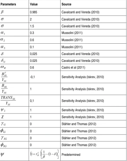
5. Calibrated parameters, prior and posterior

In this section we pursue a two-tier approach: the parameters not directly related to the questions which we endeavor to answer throughout this article are calibrated, while those relevant parame-ters for the analysis of the shock propagation are estimated using the Bayesian methodology. The main calibration procedure employed here is to pick up the values of parameters from other relevant arti-cles in the DSGE model literature. Table 2 summarizes the calibra-tion of the parameters.

Table 1 - Observables variables of the model

Variable Series Source

P Series constructed using the IPCA (\%a.m.) IBGE/SNIPC TRANS Benefícios assistenciais (LOAS e RMV) R\$ (milhões)} Min. Fazenda/STN RTL IR - pessoas físicas R\$ (milhões) Min. Fazenda/SRF RTKp IR - pessoas jurídicas R\$ (milhões) Min. Fazenda/SRF RTC ICMS and IPI R\$ (milhões) Min. Fazenda/SRF

B

R Selic Over (\% a.m.) BCB Boletim/M. Finan. Y PIB - preço de mercado - R\$ (milhões) IBGE/SCN 2000 Trim. G Consumo inal - adm. pública - R\$ (milhões) IBGE/SCN 2000 Trim. C Consumo inal - famílias - R\$ (milhões) IBGE/SCN 2000 Trim. X Exportações - R\$ (milhões) IBGE/SCN 2000 Trim. IMP Importações - R\$ (milhões) IBGE/SCN 2000 Trim. L Horas pagas - indústria geral - índice (jan. 2001 = 100) PIMES/IBGE

F

R Estados Unidos - taxa de juros (\% a.a.) Fundo Monetário Internacional, International Financial Statistics

S Taxa de câmbio - R\$ / US\$ - comercial - compra - média

Banco Central do Brasil, Boletim, Seção Balanço de Pagamentos (BCB Boletim/BP)

Table 2 - Calibration of the Parameters

Parameters Value Source

β 0.985 Cavalcanti and Vereda (2010)

σ 2 Cavalcanti and Vereda (2010)

σ 1.5 Cavalcanti and Vereda (2010)

1

α 0.3 Mussolini (2011)

2

α 0.6 Mussolini (2011)

3

α 0.1 Mussolini (2011)

δ 0,025 Cavalcanti and Vereda (2010)

G

δ 0.025 Cavalcanti and Vereda (2010)

R

ω 0.6 Castro et al (2011)

SS F SS

Y B

-0,1 Sensitivity Analysis (Iskrev, 2010)

SS SS

Y B

1 Sensitivity Analysis (Iskrev, 2010)

SS SS

Y TRANS

0,1 Sensitivity Analysis (Iskrev, 2010)

2

ψ 1 Sensitivity Analysis (Iskrev, 2010)

χ 1 Sensitivity Analysis (Iskrev, 2010)

G

γ 0 Stähler and Thomas (2012)

G

φ 0 Stähler and Thomas (2012)

IG

γ 0 Stähler and Thomas (2012)

IG

φ 0 Stähler and Thomas (2012)

ψ

(

)

( )

  

 

− −

+ δ

β

τ 1 1

1 C S

S Predetermined

Source: Own calculations.

Iskrev (2010) provides a method for testing the set of combination of parameters’ values in order that Blanchard and Kahn (1980) con-ditions are met. Subsequently, from this set of values the procedure was to choose those values for the parameters that fulfill the con-ditions which are considered standard in the literature. As in 2014 the public sector net external debt was around -10% of GDP, the

parameter

SS F SS

Y B

the ratio public debt to GDP a value of 200%. In our view, the latter value is perhaps too high, so we opt to be more conservative and use

SS SS

Y B

(ratio public debt to GDP a value of 100%).

Obtaining the average value of total transfers from the government to households is by no means an easy task. This is why we rec-kon that a value of 10% as a percentage of GDP would be more

than acceptable _

  

 

=0.1

.

SS SS

Y TRANS

. As regards the parameters ψ2 and

χ

, since they are not fiscal-policy-related variables, we decided to normalize these parameters to 1.

The parameters

γ

G,

φ

G,

φ

IG and

γ

IG were set at zero, following Stahler and Thomas (2012). This choice implies that fiscal policy reacts through changes in taxes, and not through changes in govern-ment spending. This seems to be the case in key episodes of recent Brazilian economic history. For instance, at the outset of the Real plan, the fiscal consolidation process mainly rested on the CPMF (Temporary Tax on Financial Transactions, Contribuição Provisória sobre Movimentação Financeira in Portuguese).4 Given the prior dis-tributions of the parameters, we estimate the posterior disdis-tributions using a Markov chain process via the Metropolis-Hastings algorithm with 100.000 iterations, a scale value 0.3 to be used for the jumping distribution, and 10 parallel chains for Metropolis-Hastings algori-thm.5 The results of the Bayesian estimation are shown in Table 3 and Figure 1.

These graphs are especially relevant in that they present key results, but they can also serve as tools to detect problems or build addi-tional confidence in one’s results. First, the prior and the posterior distribution should not be excessively different from one another. Second, the posterior distributions should be close to normal, or at least not display a shape that is clearly non-normal. Third, the green mode should not be too far away from the mode of the posterior distribution. Overall, it is worth pointing out that the estimates proved to be quite satisfactory.

4 _{See Giambiagi (2008, 2009).} 5

Table 3 - Posterior distribution of the model

Parameter prior mean post. mean 90\% HPD interval prior pstdev

C SS

τ

0.160 0.1640 0.1519 0.1760 beta 0.0100 L

SS

τ

0.170 0.1772 0.1694 0.1855 beta 0.0100 K

SS

τ

0.080 0.0616 0.0528 0.0702 beta 0.0100

TRANS

γ

0.500 0.5614 0.4560 0.6900 beta 0.1000

C τ

γ

0.500 0.7303 0.6409 0.8369 beta 0.1000

L τ

γ

_{0.500 0.5166 0.4244 0.6037 beta 0.1000}

K τ

γ

0.500 0.4959 0.3764 0.6131 beta 0.1000

TRANS

φ -0.500 -0.2750 -0.5127 -0.0897 unif 0.2887

C τ

φ

0.500 0.5632 0.2802 1.0000 unif 0.2887

L

τ

φ 0.500 0.0163 0.0000 0.0404 unif 0.2887

K τ

φ

0.500 0.0374 0.0000 0.0794 unif 0.2887

BF

χ

-0.003 -0.0045 -0.0050 -0.0039 unif 0.0014

X

γ 0.500 0.5042 0.3953 0.6010 beta 0.1000

X

φ 0.500 0.1456 0.0000 0.3211 unif 0.2887

D

ω 0.850 0.8364 0.8240 0.8493 beta 0.0100

D

ψ 5.000 3.2352 2.8044 3.6456 gamma 0.5000

INSD

φ

0.850 0.8787 0.8280 0.9330 beta 0.0500

θ 0.750 0.7445 0.7285 0.7587 beta 0.0100

W

θ 0.750 0.7535 0.7443 0.7638 beta 0.0100

ψ

10.000 13.0704 8.7269 18.4005 gamma 5.0000

W

ψ

10.000 15.4805 9.2004 27.2836 gamma 5.0000

C

φ

0.800 0.7957 0.7850 0.8052 beta 0.0100

R

γ 0.500 0.3262 0.2338 0.4251 beta 0.1000

Y

γ 0.500 0.4530 0.3985 0.5070 gamma 0.0500

π

γ

3.000 3.0646 2.9539 3.1823 gamma 0.1000

a

ρ 0.500 0.5549 0.4837 0.6312 beta 0.1000

G

ρ 0.500 0.4751 0.3675 0.5866 beta 0.1000

IG

ρ 0.500 0.5187 0.4288 0.6076 beta 0.1000

TRANS

ρ 0.500 0.5713 0.4729 0.6780 beta 0.1000

C

τ

ρ 0.500 0.5450 0.4274 0.6552 beta 0.1000

L

τ

ρ 0.500 0.3698 0.2677 0.4684 beta 0.1000

K

τ

Table 3 - Posterior distribution of the model - (continuation)

Parameter prior mean post. mean 90\% HPD interval prior pstdev

m

ρ 0.500 0.5450 0.3892 0.7256 beta 0.1000

P

ρ 0.500 0.4334 0.3665 0.5150 beta 0.1000

L

ρ _{0.500 0.4571 0.3523 0.5652 beta 0.1000}

I

ρ 0.500 0.6123 0.5276 0.7025 beta 0.1000

X

ρ _{0.500 0.4939 0.3838 0.6053 beta 0.1000}

RF

ρ 0.500 0.5828 0.4928 0.6684 beta 0.1000

PF

ρ 0.500 0.7764 0.6953 0.9045 beta 0.1000

ε

1.0 0.1321 0.1176 0.1476 invg Inf

G

ε

1.0 0.1308 0.1176 0.1452 invg Inf

IG

ε

_{1.0 1.3021 0.9808 1.7152 invg Inf}

TRANS

ε

1.0 0.5577 0.2982 0.7773 invg Inf

C τ

ε

1.0 0.2236 0.1620 0.2732 invg Inf

L τ

ε

1.0 0.1827 0.1504 0.2129 invg Inf

K τ

ε

1.0 0.2195 0.1798 0.2587 invg Inf

m

ε

1.0 0.1272 0.1176 0.1383 invg Inf

P

ε 1.0 0.3266 0.1955 0.4582 invg Inf

L

ε 1.0 0.4286 0.2229 0.6244 invg Inf

I

ε 1.0 0.5671 0.4055 0.7249 invg Inf

X

ε 1.0 0.1386 0.1176 0.1561 invg Inf

RF

ε

_{1.0 0.1267 0.1176 0.1377 invg Inf}

PF

ε

_{1.0 0.1468 0.1214 0.1691 invg Inf}

6. Results

This section analyzes the dynamic properties of the model by fo-cusing on the shocks decomposition of the GDP and the fiscal multipliers.

6.1. Shocks decomposition

One way to assess the effects of the different shocks on GDP fluc-tuations is to look into the decomposition of these shocks (Figure 2). Two variables were found relevant in accounting for the output behavior: current spending and public investment. Both performed similarly, reducing output over the period 2003 to 2006, as a strong fiscal adjustment was under way. However, during the period in which the Growth Acceleration Programs (PAC, in Portuguese) pre-vailed - PAC1 and PAC2 were initiated in 2007 and 2010, respec-tively -, government expenditure and public investment played an important role in boosting aggregate demand.

6.2. Fiscal multipliers analysis

In this section, we turn to gauging the fiscal multipliers for each fiscal shock (Figure 3). The results are in accordance with what was presented in Section 2, namely, in the small-economy case the multipliers should be smaller than 0.5 - it is worth remarking that these would be even smaller if there were a pressing need to put the fiscal house in order to keep public debt stable (Spilimbergo

et al., 2009). The greatest multiplier found in this work was that

of the consumption-tax excise reduction. Its associated value was 0.09 on impact, reaching 0.12 at 8 periods, with this number falling steadily over 16 quarters on the grounds of the need to adjust other fiscal tools, since the falling tax revenues led to a growing public debt (perceived effect by MOURA (2015) and by CAVALCANTI and SILVA (2010)). This growth was, however, temporary and the multiplier resumed growing.

preceding multiplier), bottoming out at 0.04 and then bouncing back thereafter until reaching a stable level. Concerning the public-in-vestment multiplier, its value on impact was smaller than the earlier figures, 0.003, it thereon embarked on a downward path (thereby mimicking somehow the behavior of the prior fiscal measures’ mul-tipliers) but its upward trajectory after the rebounding was steeper than those of the previous fiscal policies. The reason is that a po-sitive shock to public investment renders firms more productive as the higher investment turns into capital stock (In the same way as in MOURA (2015)).

The only income-tax measure yielding a positive multiplier is the tax exemption from labor income. On impact, the value was modest - 0.005 -, but in the longer run this number improved due to the increase in the households’ labor supply. The same policy applied to capital income gave rise to a negative result at any horizon.

Figure 2 - GDP Shocks Decomposition

Figure 3 - Fiscal multipliers for each fiscal shock

Source: Own calculations.

7. Conclusions

This article intended to make a contribution to the discussion about the effects of the Brazilian fiscal policy after the 2008 crisis. In this vein, a shocks decomposition for Brazilian GDP as well as a multi-plier analysis of each fiscal shock were undertaken under the fra-mework of a New Keynesian model. The spending-based measures were the most successful in affecting GDP over the whole period studied, primarily because of PAC2, whose actual goal was to bolster aggregate demand. However, this stimulus program had a positive result until 2013, thereafter the deterioration of this type of fiscal policy negatively affected the Brazilian economic result.

Bibliography

BATINI, N., EYRAUD, Luc and WEBER, A. A Simple Method to Compute Fiscal Multipliers. IMF Working Paper No. 14/93; June, 2014.

BLANCHARD, O. J. and KAHN, C. M. The Solution of Linear Difference Models under Rational Expectations. Econometrica, Econometric Society, vol. 48(5), pages 1305-11, July, 1980. CALVO, G. Staggered Prices in A Utility-Maximizing Framework. Journal of Monetary Economics,

12, p. 383-398, 1983.

CANOVA, F. Methods for Applied Macroeconomic Research. New Jersey: Princeton University Press. 492 p, 2007.

CARVALHO, F. A., and VALLI, M. An estimated DSGE Model with Government Investment an Primary Surplus rule: the Brazilian case. $32^0$. Encontro da SBE, Salvador: SBE, 2010. Available in: http://bibliotecadigital.fgv.br/ocs/idex.php/sbe/EBE10/paper/view/2141/1061. Accessed on: February

14, 2016.

CASTRO, M. R., GOUVEA, S. N., MINELLA, A., SANTOS, R. and SOUZA-SOUBRINHO, N. F. SAMBA: Stochastic analytical model with a bayesian approach. Banco Central do Brail. Working Papers Series n. 29, p. 1-138, 2011. In: hhttp://bcb.gov.br/pec/wps/ingl/wps239.pdf. Acesso em: 02 out 2013.

CAVALCANTI, M. A. F. H., and VEREDA, L. Propriedades dinamicas de um modelo DSGE com parametrizacoes alternativas para o Brasil. Ipea, Texto para Discussão, n 1588, 2010.

CAVALCANTI, M. A. F. H. and SILVA, N. L. C. Dívida pública, política iscal e nível de atividade: uma

abordagem VAR para o Brasil no período 1995-2008. Economia Aplicada, 14(4), 391-418, 2010. CAVALCANTI, M. A. F. H., and VEREDA, L. (in press). Fiscal Policy Multipliers in a DSGE Model

for Brazil, 2016. Available in: http://bibliotecadigital.fgv.br/ojs/index.php/bre/article/view/57570. Accessed on: February 14, 2016.

CHRISTIANO, L., EICHENBAUM, M. and REBELO, S. When is the government spending multiplier large? NBER working paper series, working paper 15394, 2009.

DEJONG, D., N., and DAVE, C. Structural Macroeconometrics. New Jersey: Princeton University Press. 338 p., 2007.

DIXIT, A. K. and STIGLITZ, J. E. Monopolistic competition and optimum product diversity. The American Economic Review, 67, p. 297-308, 1977.

FANTINATTI, A. M. Estímulos iscais em um modelo DSGE: bens duráveis versus bens não duráveis.

Dissertação de Mestrado Proissional. Fundação Getúlio Vargas - Escola de Economia São Paulo,

2015.

GIAMBIAGI, F. 18 anos de política iscal no Brasil: 1991/2008. Economia aplicada, 12(4), 535-580, 2008.

___________. A política iscal do governo Lula em perspectiva histórica: qual é o limite para o aumento

do gasto público? Planejamento e políticas públicas, (27), 2009.

ILZETZKI, E., MENDOZA, E.G. and VÉGH, C.A. How big (small?) are iscal multipliers? Journal of

Monetary Economics, 60, p. 239-254, 2013.

ISKREV, N. Local identiication in DSGE models, Journal of Monetary Economics, 57(2), 189–202, 2010.

MENDONÇA, M. J. C., MEDRANO, L. A. and SACHISIDA, A. Avaliando a Condição da Política Fiscal no Brasil. Revista de Economia e Administração (Impresso), v. 9, p. 294-316, 2010.

MOREIRA, T. B. S. A crise inanceira internacional e as políticas anticíclicas no Brasil. 2010. Disponível

em: <www.tesouro.gov.br>.

MUSSOLINI, C. C. Ensaios em política iscal. Tese de Doutorado (Doutorado em Economia de Em-presas) Fundação Getúlio Vargas - Escola de Economia São Paulo, 2011.

PERES, M. A. F. and ELLERY JR., R. G. Efeitos dinâmicos dos choques iscais do governo central do

PIB do Brasil. Pesquisa e Planejamento Econômico, 39(2), 159-206, 2009.

SCHMITT-GROHÉ, S., and URIBE, Martín. Closing small open economy models. Journal of Interna-tional Economics, 61, pg 163-185, 2003.

SPILIMBERGO, A., SYMANSKY, S. and SCHINDLER, M. Fiscal Multipliers. IMF Staff position note 2009/11 (Washington: International Monetary Fund), 2009.

STÄHLER, N., and THOMAS, C. FiMod—A DSGE model for iscal policy simulations. Economic Modelling, 29(2), 239-261, 2012.

ZUBAIRY, S. On iscal multipliers: estimates from a medium scale DSGE model. International Economic Review, v. 55, issue 1, p. 169-195, 2014.

WOODFORD, M. Simple analytics of the government expenditure multiplier. American Economic