A Work Project, presented as part of the requirements for the Award of a Master Degree in Finance from Nova School of Business and Economics
NYSE Decimalization: The Impact on Holding Periods
Talita Alves Barbosa, nº 2303
A Research Project carried out under the supervision of:
2 Abstract
The recent decrease in average stock holding periods has drawn growing attention from market participants. As empirical studies provide evidence of narrower bid-ask spreads and transaction costs after the decimalization, it begs the question of whether the reduction of tick sizes has, in fact, decreased the holding period of stocks. Using data from 2,601 NYSE-listed stocks, we investigate the impact of the decimalization on the holding period of common stocks by institutional investors. The results show that after the decimalization, holding periods are shorter, as investors trade 78.9 percent more frequently than before.
3 1. Introduction
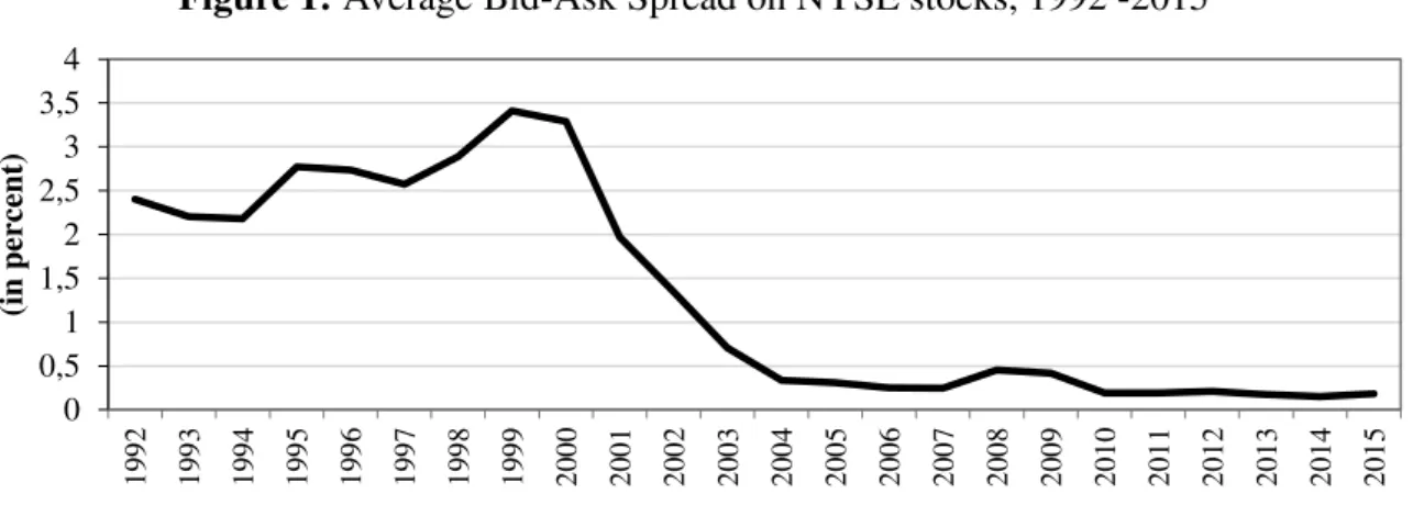
Over the last decades, stock bid-ask spreads have fallen dramatically across financial markets. In the New York Stock Exchange (NYSE) alone, average spreads have decreased by approximately 40 and 94 percent in the last 10 and 20 years, respectively (see Figure 11). Many practitioners refer to the reduction in tick size as one of the main reasons of these lower spreads. Narrower spreads are closely related to lower trading costs that can foster more trading activity and, as consequence, shorten investors’ holding periods. Given the short-term nature of much of the trading decisions today, the goal of this thesis is to study the impact of the decimalization on the holding periods of NYSE common stocks by institutional investors.
The historical decreasing trend in average spreads is linked to the decline in transaction costs faced by investors. Simply put, bid-ask spread is the difference between the price a buyer is willing to pay (bid price) and the price a seller is willing to accept (ask price) to sell a given stock. This price difference constitutes a hidden transaction cost that, along with brokerage commission, fees, and taxes, directly impacts the return for an investor. Consequently, a decrease in spreads is expected to decrease trading costs and can have a significant impact in trading frequency.
1 The data presented corresponds to the average of daily-bid ask spread over each year. Data for bid and ask prices were retrieved from the Center for Research in Security Prices (CRSP).
0 0,5 1 1,5 2 2,5 3 3,5 4 1 9 9 2 1 9 9 3 1 9 9 4 1 9 9 5 1 9 9 6 1 9 9 7 1 9 9 8 1 9 9 9 2 0 0 0 2 0 0 1 2 0 0 2 2 0 0 3 2 0 0 4 2 0 0 5 2 0 0 6 2 0 0 7 2 0 0 8 2 0 0 9 2 0 1 0 2 0 1 1 2 0 1 2 2 0 1 3 2 0 1 4 2 0 1 5 (in perc ent )
4 In the NYSE, the gradual decrease of the tick size, which is the minimum change in a security’s price, started in 1997 when the tick size changed from one-eighth to one-sixteenth of a dollar and continued in 2001 with the decimalization that further reduced minimum increments to one cent per share. This has prompted smaller spreads as they can be as small as the tick size. In practical terms, after the decimalization, if an investor bought 100 shares and immediately wanted to sell them, the total transaction cost due to the spread would be of at least $1, instead of $6.25 before 2001, and $12.5 before 1997.
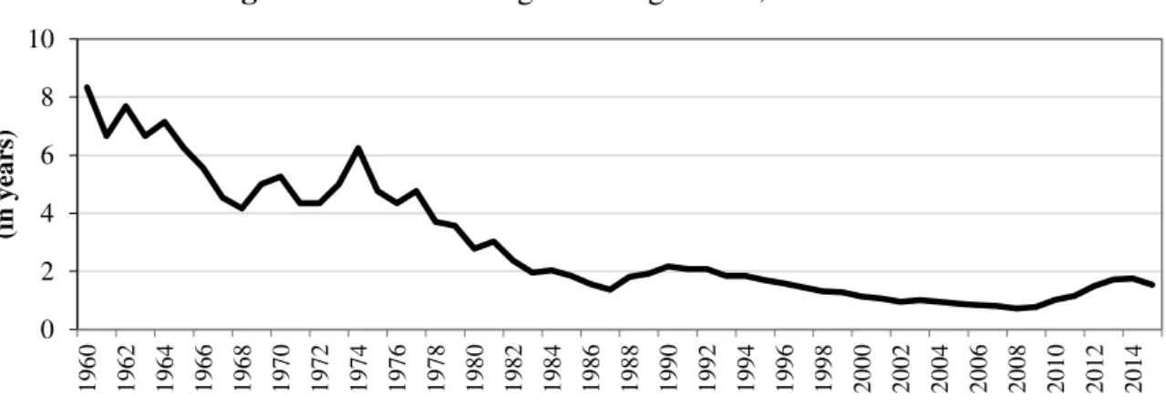
Along with the decline in bid-ask spreads, the increasing short-termism of investments decisions is also clear in the marketplace. Figure 22 presents an overview of the data regarding the average holding period of NYSE stocks. The data provides an initial benchmark for the behaviour of investors over time. Even though there are many variations before the 1990s, by looking at the overall trend, one can easily identify that stocks are being held for shorter periods in the last years. Evidently, there are other factors that have also influenced investor’s investment decisions over time, but still, the sizable decrease in bid-ask spreads begs the question of whether these narrower spreads have fostered shorter investment horizons.
2 Average holding period was calculated as the inversion of turnover which is commonly used as a simplified proxy for the average holding period. Data for turnover was collected from NYSE’s Transactions, Statistics, and Data Library.
0 2 4 6 8 10 1 9 6 0 1 9 6 2 1 9 6 4 1 9 6 6 1 9 6 8 1 9 7 0 1 9 7 2 1 9 7 4 1 9 7 6 1 9 7 8 1 9 8 0 1 9 8 2 1 9 8 4 1 9 8 6 1 9 8 8 1 9 9 0 1 9 9 2 1 9 9 4 1 9 9 6 1 9 9 8 2 0 0 0 2 0 0 2 2 0 0 4 2 0 0 6 2 0 0 8 2 0 1 0 2 0 1 2 2 0 1 4 (in y ea rs)
5 There is extensive literature about the implementation of the decimalization in the NYSE. These work studies find that the tick size reduction increased liquidity and influenced trading volume in the market. While it has been found that the smaller tick size has increased the overall trading volume in the market, to the best of our knowledge, there is no research dedicated to measuring the impact of the decimalization on the holding period of these stocks. Using a duration analysis, we study average holding periods by institutional investors pre- and post-decimalization while controlling for bid-ask spreads, returns, market value and
volatility of a firm’s stock, as well institutional investor’s type and country of residence. We
find evidence for shorter holding periods after the decimalization as institutional investors show an increase of 78.9 percent in their hazard rate. The negative effect on holding periods is
confirmed over different window sizes, and is shown to vary in size depending on investor’s
characteristics.
The structure of this thesis is as follows. Section 2 discusses previous literature related to the 2001 decimalization as well as other work studies regarding the determinants of holding periods. The data and methodology used are presented in Section 3, which is followed by the model results in Section 4. Finally, Section 5 provides some concluding remarks.
2. Literature Review
I. The Decimalization and its Impact in Market Behaviour
6 smaller pricing increments – tick size – to listed securities, in 1997 and 2001 (See Matheson (2011)).
This study will focus on the latter event which put an end to the tradition of pricing stocks under a fractional system. The decimalization has spurred a large number of academic literature that investigate the extent to which the tick size reduction affected liquidity and trading behaviour. When investigating the impact of the decimalization, many studies have found that that the smaller price increments have indeed been used in the market, therefore prompting smaller bid-ask spreads (e.g., Chakravarty, Harris, Wood (2001), Bacidore, Battalio and Jennings (2003), and Bessembinder (2003)).
Regarding the impact on trading volume, the evidence is mixed. Chakravarty, Wood, and Van Ness (2004) find that the introduction of penny increments had a negative impact in trading volume for all trade sizes. In a more recent study, however, Chakravarty, Van Ness, and Van Ness (2005) come to the conclusion that small order sizes are the ones trading more actively after decimalization, while trading activity has reduced for larger order sizes.
Since institutional investors are the main responsible for larger transactions, it is suggested that retailers were favoured at the expense of institutional traders. Yet, it should be considered that institutions are informed traders and, as such, may adapt their trading behaviour to these policy changes. In fact, Oppenheimer and Sabherval (2003) show that there is an overall decline in U.S. order size after the decimalization. Thus, it is likely that institutional investors were encouraged to break up their large orders into small blocks as a response to the new decimal pricing system. This is one of the main points where our study differs from previous
literature. By having access to institutional investor’s holdings, our results take into account all
7 II. The Determinants of Holding Period for Common Stocks
When studying the impact of decimalization on the holding period, it is important to take into consideration the many determinants that may influence holding periods so as to control for confounding factors.
Primary work studies related to the time length of investment decisions suggest the relationship between bid-ask spreads and investors expected holding periods. Amihuld and Mendelson (1986) and Constantinides (1986) find that as transaction costs rise, investors tend to trade less and increase their holding period so that they can amortize their costs over a longer period of time.
Atkins and Dyl (1997) reinforce the proposition that the holding period is an increasing function of transaction costs, and finds two additional associations, suggesting that holding
periods increase with firm size and decreases with a stock’s volatility. In their study, Atkins
and Dyl (1997) use a regression analysis that has caused several researchers such as Næs and Ødegaard (2008) and Dias and Ferreira (2004) to argue that, in the case of holding period, the appropriate econometric framework should be a duration analysis. This method is argued to be more complete as it can model one’s decision to terminate a relationship, in this case, a specific
stock’s holding period.
8 3. Data and Methodology
I. Institutional Investors and Individual Stocks Data
The data for institutional investors was obtained from the Thomson Reuters Institutional Holdings (13F) Database which reported, for each investor, information about the number of shares held in each stock at the end of each quarter. This database also provided additional
investors’ characteristics such as the type of institution and country of residence. The sample
period runs from June, 2000 to September, 2001.
For each institution and in every quarter, we calculate the investor’s relative holdings in each stock. This percentage is calculated over the total shares outstanding of the stock’s firm. Whenever there is a change in relative holdings from quarter 𝑡 + 1 to quarter 𝑡, a change in holdings is identified. In the end, holding period is expressed in quarters and corresponds to the difference between quarter 𝑡 and the initial quarter that same relative holding was recorded.
We exclude all left-censored observations, i.e., stock positions for which a change in holdings occurred prior to the stock entering the study. Also, the sample period is defined so that we can have a similar proportion of observations before and after the event. The final sample consists of 49% of observations before the event. Table 1 provides information on the holdings of institutional investors. Our dataset contains a total of 401,190 quarterly holdings in 2,601 NYSE-listed stocks by 2,029 institutional investors that are actively trading during the sample period. The average holding period for all investors is 1.198 quarters before the decimalization, and 1.251 quarters afterwards.
9 the decimal pricing system. The same results are found for institutions from different countries, except from the Rest of the World.
Stock characteristics are of great importance and should be included in the model since they are expected to influence individual investment lengths. By adding these variables, we control for other factors that may have affected holding period around the decimalization. For each stock held by institutional investors, stock characteristics were obtained from the Center for Research in Security Prices (CRSP). The original data includes daily bid and ask prices, stock returns and shares outstanding for all NYSE-listed issues trading from June 1, 2000 to September 30, 2001. From this sample, we exclude all stocks that were part of the decimal pilot so that our results solely display the decimalization effect.
In line with the disposition effect presented by Shefrin and Statman (1985), investors are expected to react more quickly to positive than negative returns. That is, as they believe prices eventually convert to the mean, their holding periods are expected to decrease as returns increase. Stock return in each quarter is estimated through the annualized return that is calculated using the daily observations provided by CRSP. These returns include cash adjustments.
We also include stock’s return volatility in our model, which is estimated by the
annualized sample standard deviation of daily returns over each quarter. As volatility is mainly related to information asymmetry, its increase is expected to induce more trading and, as consequence, shorten holding periods.
10
𝐵𝑖𝑑 − 𝐴𝑠𝑘 𝑆𝑝𝑟𝑒𝑎𝑑𝑖𝑇 = [∑ 𝐴𝑠𝑘𝑖𝑡 − 𝐵𝑖𝑑𝑖𝑡
(𝐴𝑠𝑘𝑖𝑡 + 𝐵𝑖𝑑𝑖𝑡
2 )
𝑁
𝑡=1
] /𝑁 , (1)
where 𝐴𝑠𝑘𝑖𝑡 and 𝐵𝑖𝑑𝑖𝑡 are the ask and bid prices for stock 𝑖 in day 𝑡, and 𝑁 the total number of trading days for stock 𝑖 in quarter 𝑇.
Following Atkins and Dyl (1997), we also add the market value of the firm’s common
stock as a control variable, given that it is expected to negatively impact holding periods. This variable is calculated at the end of each quarter 𝑇 and for each stock 𝑖 as the product of total shares outstanding and share price.
II. Econometric Framework
Trading volume in equity markets is usually a good indicator of stocks’ holding period. In fact, when studying the impact of transaction costs on holding periods, Atkins and Dyl (1997) use the ratio between shares outstanding and trading volume as a proxy for average holding periods. Although being a simple approach that is easy to implement in a regression analysis, the total trading volume does not account for the fact that some stocks may trade very infrequently, thus having longer holding periods than other stocks that trade more often. Neither does it allow for cross-sectional comparisons at the individual level, such as across investors and stocks. Moreover, the use of a regression analysis is not appropriate for studying holding periods since they express a survival time, e.g., the duration of time over which a change in holdings is not observed. A traditional regression is not effective because data is often censored (incomplete information) and not normally distributed. To this extent, in our model specification, we follow the contemporary work of Næs and Ødegaard (2008) and Dias and Ferreira (2005), and use a duration (or survival) analysis.
11 of unemployment duration. Duration analysis can be used to estimate the survival function,
𝑆(𝑡), or the hazard function, 𝜆(𝑡). The survival function expresses the probability distribution of surviving beyond a given time 𝑡, while the hazard function is a conditional failure rate that expresses the probability per unit of time for a failure to occur, given that it has not occurred up until a given time 𝑡. The relationship between the two functions is as follows:
𝜆(𝑡) = lim∆𝑡→0𝑃(𝑡 ≤ 𝑇 < 𝑡 + ∆𝑡 |𝑇 ≥ 𝑡)∆𝑡 =𝑓(𝑡)𝑆(𝑡) , (2)
where 𝑓(𝑡) expresses the density function of survival time. In our analysis, given that
investors’ holding is only available at the end of each quarter, this rate is approximated to the
probability of the event (e.g., change in holdings) happening in quarter 𝑡, given that it has not occurred since a base period (e.g., the quarter with the last recorded change in holdings).
One of the most important applications of the duration analysis comes from the
modelling of hazard function under the Cox’s proportional hazards framework. The
proportional hazards technique models 𝜆(𝑡) while considering several explanatory variables simultaneously.
Following Dias and Ferreira (2005), we call 𝑡 the calendar time in quarters, and 𝑡̅̅̅𝑖𝑗 the calendar time at which investor 𝑖 first reaches a given position in stock 𝑗. Thus, the investor’s holding period in quarters corresponds to 𝜏 = 𝑡 − 𝑡̅̅̅𝑖𝑗. According to the Cox regression model, the hazard rate in quarter 𝑡 for stock 𝑖 and investor 𝑗 can be modelled as:
𝜆𝑖𝑗(𝑡̅̅̅ + 𝜏, 𝜏) = 𝜆𝑖𝑗 0(𝑡̅̅̅ + 𝜏, 𝜏)× exp(𝑥𝑖𝑗 𝑖′𝛽𝑖+ 𝑤𝑗𝑡′𝛽𝑗) , (3)
where 𝜆0 is the baseline hazard function3, 𝑥𝑖 the vector of fixed investor characteristics, and 𝑤𝑖𝑗 the vector of time-varying stock characteristics. The baseline hazard function and the
12
covariates’ coefficients are estimated using Breslow’s partial log-likelihood function. This
method is semi-parametric, given that 𝜆0 is an unspecified function under the Cox model.
A very important aspect underlining the Cox model is its assumption of proportional hazards. It is assumed that two different strata (i.e., two different subjects A and B who differ in their individual stock and investor characteristics) have hazard functions that are proportional over time. Given the proportionality assumption, the Cox model estimates a relative hazard rate, which is called hazard ratio, 𝐻𝑅.
𝐻𝑅𝐴,𝐵 =𝜆𝑖𝑗 𝐴(𝑡
𝑖𝑗
̅̅̅ + 𝜏, 𝜏) 𝜆𝐵𝑖𝑗(𝑡
𝑖𝑗
̅̅̅ + 𝜏, 𝜏) = exp [(𝑥𝑖𝑡𝐴 − 𝑥𝑖𝑡𝐵)
′
𝛽𝑖] . (4)
If the hazard ratio is greater than 1, the risk of changing relative holdings is increased for subject A compared to subject B. It is important to note that holding periods are intrinsically related to hazard rates, meaning that in this case subject A would be expected to show a shorter holding period.
When examining the proportionality assumption of our fixed covariates, we consider one common approach suggested by Cox. For each fixed covariate, we create an artificially time-dependent variable, which is added to the model, as follows:
𝜆𝑖𝑗(𝑡̅̅̅ + 𝜏, 𝜏) = 𝜆𝑖𝑗 0(𝑡̅̅̅ + 𝜏, 𝜏)× exp (𝑥𝑖𝑗 𝑖′𝛽𝑖+ 𝑤𝑗𝑡′𝛽𝑗+ 𝛾𝑥𝑖′𝑔(𝑡)) . (5)
If the proportionality assumption holds for the fixed covariates, there should be no change in their impact on outcome over time. Therefore, the time-dependent variable, 𝑥𝑖′𝑔(𝑡), should be statistically insignificant.
4. Results
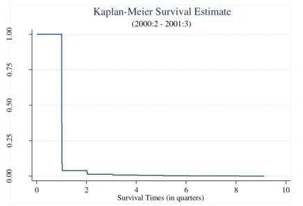
13 rates from 2000:2 to 2001:3 using the Kaplan-Meier estimator. This method is appropriate because it considers the presence of right-censored observations in our dataset (i.e., the existence of observations/funds that might not experience failure/change in holdings before the end of the study).
Figure 3: Survival Function for Holding Periods
Figure 3 plots the overall survival function of holding periods, with no covariates involved, for the entire sample period. The survival rate drops substantially in the first quarter, suggesting a fast increase in the hazard rate after an investor holds a stock during a whole quarter. This strong decline is likely related to the fact that, in many cases, institutions do not hold a stock for an entire quarter. As expected, changes in holdings are most likely to occur in the first periods. At longer periods of time, the survival rate approaches zero survival probability suggesting that fewer investors keep the same position. As we are interested in testing whether the holding period changed after the decimalization, we test the equality of survival times pre- and post-decimalization. To formally test this difference, we first estimate the survival function before and after the decimalization event, and then perform the log-rank test, which tests the null hypothesis that there is no difference between the two population
0.
00
0.
25
0.
50
0.
75
1.
00
0 2 4 6 8 10
Survival Times (in quarters)
(2000:2 - 2001:3)
14 survival curves. After performing this test, we find that in fact there is a statistically significant difference between the two survival curves (p < 0.001).
As a way of fully understanding the impact of the decimalization, we follow the Cox proportional hazards model approach to estimate the size of the difference in the holding periods pre- and post-decimalization. For this purpose, we study different model specifications. First, we estimate our base model which contains all control variables used in our study. Next, the base model is extended to include the event effect of the decimalization, which is again estimated through different window sizes as a way of validating our results. The effect of the decimalization is finally compared among institutions depending on their type and country of residence.
In all model specifications estimated in this study, we start by checking the proportionality assumption when fitting the Cox model to ensure the validity of our results. After adding a time-dependent variable for each fixed covariate, we check if they are statistically significant. Whenever the time-dependent variable is significant, we have a problem of non-proportionality. As a solution to this problem, we keep the time-dependent variable in the model, and relax the PH assumption by extending the Cox model. In the case of the time-varying covariates (bid-ask spread, annualized return, standard deviation of returns and market value), the hazards are clearly not constant over time given that they depend on the values of the covariates at each period 𝑡. As we are interested in studying the overall impact of decimalization in holding periods and since the hazard model is reasonably robust, we follow
Allison (2005) by interpreting the results of these variables’ coefficients as their “average”
effect over the period of observation.
15 model, we group the data depending on their stock. By doing this, we adjust standard errors, and account for the correlation that may exist between them.
I. Description of the Base Model
Table 3 presents the hazard ratios estimated for the different model specifications. The estimates for the base model are in column (1), and correspond to the main sample period from 2000:2 to 2001:3. This model includes only the control variables: bid-ask spread, annualized return, standard deviation of returns, market value and investors characteristics that are divided by type of institution and country of residence.
In the base model, the bid-ask spread is statistically significant and has an estimated hazard ratio of 0.9161, meaning that an increase of 1 percent in the spread relates to a decrease of 8.39 percent in the hazard rate, ceteris paribus. If the hazard rate decreases with the spread, so does the probability of changing holdings. Thus, this finding is in accordance with Dias and Ferreira (2005) and Atkins and Dyl (1997) as it translates a negative relation between spread and holding periods. Holding periods are also found to increase as stock returns increase. This finding is contrary to the disposition effect theory, which states that investors sell winners more quickly than they sell loser stocks. In fact, our results are consistent with O’Connell and Teo (2009), who find that large institutional investors, unlike individual investors, are more likely to sell their holdings after experiencing losses. Finally, stock returns’ volatility and firm size are estimated to have a negative effect on holding periods. These results are in line with previous literature, suggesting that investors are prone to trade more frequently in relatively larger firms and for stocks with higher volatility. Even though the effect of these variables on holding period appears to be small (hazard ratio close to 1), it should be noted that the
coefficients are in accordance with the covariates’ units, i.e., they translate a change of 1 percent
16
The role of institutional investors’ characteristics will be analysed further in this study
using a stratified Cox model.
II. Evidence for Shorter Holding Periods after the Decimalization
As a way of assessing the difference in holding periods pre- and post-decimalization, we extend our model specification to include a dummy variable for the decimalization event that takes the value of 0 before the decimalization event, and 1 thereafter. The interpretation of the event variable becomes simple since a hazard ratio greater than 1 will signal a higher rate of transition in holdings, and consequently shorter holding periods post-decimalization. Column (2) of Table 3 presents our results for the full model. While controlling for possible confounding effects, we find that after the decimalization institutional investors present a transition rate that is 78.9 percent higher than before the reduction in tick sizes. Consistent with our hypothesis, this result provides evidence for narrower holding periods among institutional investors. This increased hazard rate can be illustrated in the example of Capital City Trust
Company’s holdings on Oklahoma Gas & Electric (OGE) stock. For this specific case, the
investor keeps the same stock position in all periods before the decimalization. After the tick size reduction, however, stock positions are changed 33% of the time.
17 decrease this rate of transition. For instance, the hazard ratio is suggested to increase by “only” 61.35 percent, if one considers 6 quarters pre- and post-decimalization. The ability of institutional investors to adjust their trading strategies over time may explain this interesting behaviour in the long-term. Table 4 summarizes the results for all windows going from small (column (1)) to large (column (4)). As it can be seen, the effect of the decimalization is robust to different window sizes.
III. Evidence for Consistency in Results across Institutional Investors
From the previous section, there is clear evidence of portfolio rebalancing after the introduction of decimal pricing. However, it is not clear whether this phenomenon is consistent across different types of institutions and countries or if it is mostly due to the strong contribution of a specific type of investor. For that reason, we further extend our study and estimate a stratified Cox regression model. That is, we divide the overall sample into subgroups according
to institutional investors’ characteristics, which allows the baseline hazard to differ across them.
Here, our main goal is to assess the impact of the decimal system across different type of institutions and countries. The results of these models estimation are presented in Table 5.
18 When assessing the hazard of investors from different countries, the discrepancy in results is noticeably strong. The largest impact seems to be on investors from the United Kingdom, who show a hazard rate that is 98.5 percent larger than before the decimalization. Following the U.K., American investors also show a strong reaction, with a hazard 78.9 percent higher. Holding periods of investors from the Euro-zone, on the other hand, are far less affected by the decimal pricing, showing an increase in the hazard rate of only 17.7 percent. In fact, this difference in results may relate to the barriers of access to information, as the different levels of market transparency experienced by domestic and foreign investors is likely to play a role in the way they adjust their equity holdings after the decimalization.
5. Conclusion
In this research, we use a duration approach to study the impact of the NYSE decimalization on the holding period of common stocks by institutional investors. The impact on holding periods is derived from the hazard ratio, that translates the rate at which investors change their equity holdings. Some previous literature finds that institutional investors’ trading volume has declined after the reduction of tick sizes. However, their results are only based on the overall trading volume of large size orders. It is in this way that our study differs from previous research. The use of duration analysis allows us to consider not only the determinants of holding periods, but also the duration-dependence that exists in this type of data. Also, since
we have information on institutional investor’s quarterly holdings, we can account for all their
dynamic trading behaviour (i.e., possible changes in order sizes after the event).
19 shown to be stronger for shorter-term data. The size of the effect depends on investor’s characteristics, but is always found to be in accordance with the expected increase in the hazard.
It is important to note that our analysis is based on quarterly data of institutional
investors’ stock holdings. As such, we may lose some important information regarding the
hazard rate at the very short end – for holding periods shorter than 3 months. The use of monthly or even daily data would allow us to define shorter window sizes, which would likely capture a greater portion of the true effect of the decimalization in holding periods.
Since this study addresses the trading behaviour of institutional investors in the face of a regulatory change, our results should be of interest to market participants as well as to policy makers. Institutional investors, for instance, may consider how this decrease in their holding period of common stocks may affect their tax cost, given that short-term gains usually face substantially higher taxation. For market regulators, on the other hand, it can be worthwhile to examine whether the old regulation continues to be appropriate in the face of a new market structure. For instance, transaction fees can decrease with the shortening of holding periods. Since these fee rates aim at recovering the cost incurred in regulation and supervision of a stock market, the fee per transaction can decrease as the trading volume in the market increases (See Section 31 Transaction Fees (2013)). The reduction in holding periods post-decimalization (i.e., the increase in transaction volume) means that each transaction must contribute less, therefore allowing for lower fee rates in the market.
20 6. References
Allison, Paul D. 1995. Survival Analysis Using SAS: A Practical Guide. Cary: SAS Institute.
Amihud, Y., and H. Mendelson. 1986. “Asset Pricing and the Bid-Ask Spread”. Journal of Financial Economics, 17: 223-250.
Atkins, A., and E. Dyl. 1997. “Transactions Costs and Holding Periods for Common Stocks”. Journal of Finance, 52: 309-325.
Bacidore, Jeffrey, Robert H. Battalio and Robert H. Jennings. 2003. “Order Submission Strategies, Liquidity Supply, and Trading in Pennies on the New York Stock Exchange”. Journal of Financial Markets, 6(3): 337-362.
Bessembinder, Hendrik. 2003. “Trade Execution Costs and Market Quality After Decimalization”. Journal of Financial and Quantitative Analysis,38(4): 747-777.
Chakravarty, Sugato, Stephen P. Harris and Robert A. Wood. 2001. “Decimal Trading and Market Impact”. Working Paper, University of Memphis.
Chakravarty, Sugato, Bonnie F. Van Ness, and Robert A. Van Ness. 2005. “The Effect of Decimalization on Trade Size and Adverse Selection Costs”. Journal of Business Finance & Accounting, 32(5-6): 1063-1081.
Chakravarty, Sugato, Robert A. Wood and Robert A. Van Ness. 2004. “Decimals and Liquidity: A Study of the NYSE”. Journal of Financial Research, 27: 75-94.
Constantinides, G. 1986. “Capital Market Equilibrium with Transaction Costs”. Journal of Political Economy, 94: 842-862.
Dias, Jorge D. and Miguel A. Ferreira. 2005. “Timing and Holding Periods for Common Stocks: A Duration-Based Analysis”. Working Paper, ISCTE Business School.
Matheson, Thornton. 2011. “Taxing Financial Transactions: Issues and Evidence”. IMF Working Paper No. 11/54, International Monetary Fund.
Næs, Randi, and Ødegaard, Bernt. 2008. “Liquidity and Asset Pricing: Evidence on the Role of Investor Holding Period”. Working Paper, Norges Bank.
O’Connell, Paul G. J., and Melvyn Teo. 2009. “Institutional Investors, Past
Performance, and Dynamic Loss Aversion”. Journal of Financial and Quantitative Analysis, 44(1): 155-158.
Oppenheimer, Henry R., and Sanjiv Sabherwal. 2003. “The Competitive Effects of US Decimalization: Evidence from the US-listed Canadian Stocks”. Journal of Banking and Finance, 27(9): 1883-1910.
Section 31 Transaction Fees. 2013. https://www.sec.gov/answers/sec31.htm (accessed December 27, 2016)
21 Table 1
Descriptive Statistics of Holding Periods Pre- and Post-Decimalization
Number of
Observations Mean Standard Deviation
Before After Before After Change (%) Before After Change (%)
TOTAL 772,043 788,252 1.198 1.251 4.4% 0.653 0.899 37.6%
Panel A: Type of Institution
Banks 72,816 134,250 1.270 1.279 0.7% 0.760 0.923 21.5%
Insurance Companies 25,982 24,989 1.156 1.229 6.3% 0.623 0.836 34.2%
Investment Companies and Their Managers 12,710 12,658 1.181 1.123 -4.9% 0.622 0.637 2.5%
Investment Advisors 57,115 69,203 1.203 1.265 5.2% 0.660 0.899 36.2%
All Others 603,420 547,152 1.191 1.247 4.7% 0.640 0.901 40.7%
Panel B: Country of Residence
United States 735,101 745,443 1.198 1.252 4.5% 0.654 0.901 37.9%
United Kingdom 16,907 17,247 1.161 1.196 3.1% 0.542 0.736 35.8%
Canada 10,288 13,913 1.177 1.242 5.5% 0.583 0.891 52.8%
Euro-zone 690 1,378 1.055 1.195 13.3% 0.203 0.593 192.3%
Rest of the world 9,057 10,271 1.311 1.269 -3.2% 0.864 1.013 17.2%
22 Table 2
Descriptive Statistics of Stock Characteristics Pre- and Post-Decimalization
Bid-Ask Spread Quarterly Return
Number of (Percent) (x100) (Percent)
Period Observations Mean Median Std. Dev. Mean Median Std. Dev.
Full Sample 14,262 1.839% 1.205% 2.056% 0.036 0.060 1.035
Pre-Decimalization 7,209 2.507 1.926 2.330 0.082 0.103 1.002
Post-Decimalization 7,053 1.157 0.752 1.440 -0.012 0.009 1.066
Std. Dev. of Returns Market Value
Number of (x100) (Percent) (Billions)
Period Observations Mean Median Std. Dev. Mean Median Std. Dev.
Full Sample 14,262 0.432 0.378 0.288 $ 4.436 $ 0.525 $ 19.731
Pre-Decimalization 7,209 0.445 0.393 0.302 4.612 0.505 20.972
Post-Decimalization 7,053 0.418 0.364 0.272 4.257 0.544 18.375
23 Table 3
Estimates for the Hazard Rates of Holding Periods (2000:2 – 2001:3)
(1) (2)
Decimalization (0=Pre, 1=Post) 1.7887**
(95% CI) (1.7784 - 1.7990)
Bid-Ask Spread 0.9161** 0.9773**
(95% CI) (0.9059 - 0.9265) (0.9754 - 0.9793)
Annualized Return 0.9408** 0.9453**
(95% CI) (0.9247 - 0.9571) (0.9426 - 0.9479)
Std. Dev. Of Returns 1.0699** 1.1333**
(95% CI) (1.0191 - 1.1231) (1.1206 - 1.1460)
Market Value 1.0010** 1.0010**
(95% CI) (1.0006 - 1.0013) (1.0009 - 1.0010)
Type of Institution
Insurance Companies 1.0888** 1.0844**
(95% CI) (1.0746 - 1.1032) (1.0692 - 1.0999)
Investment Advisors 1.0731** 1.0862**
(95% CI) (1.0561 - 1.0904) (1.0680 - 1.1048)
Investment Companies and Their Managers 1.0502** 1.0335**
(95% CI) (1.0401 - 1.0604) (1.0235 - 1.0436)
All Others (Pension Funds, Foundations) 0.9948 0.9963
(95% CI) (0.9868 - 1.0028) (0.9898 - 1.0028)
Country of Residence
United Kingdom 0.9925 0.9931
(95% CI) (0.9774 - 1.0079) (0.9776 - 1.0089)
Canada 1.0907 1.0075
(95% CI) (1.0742 - 1.1075) (0.9906 - 1.0246)
Eurozone 0.8689** 0.7813**
(95% CI) (0.8397 - 0.8991) (0.7468 - 0.8173)
Rest of the World 0.9760** 0.9188**
(95% CI) (0.9590 - 0.9933) (0.8993 - 0.9387)
Adjustment for Non-Proportionality
in Type of Institution No No
in Country of Residence Yes No
Log Likelihood -6045190.1 -6029875.1
Number of Observations 539,479 539,479
24 Table 4
Estimates for the Hazard Rates of Holding Periods
(1) (2) (3) (4)
Decimalization (0=Pre, 1=Post) 2.6110** 1.6269** 1.5827** 1.6135**
(95% CI) (2.5776 - 2.6449) (1.6008 - 1.6535) (1.5419 - 16247) (1.5840 - 1.6435)
Bid-Ask Spread 0.9707** 0.9782** 0.9568** 0.9586
(95% CI) (0.9684 - 0.9731) (0.9696 - 0.9868) (0.9465 - 0.9673) (0.9483 - 0.9691)
Annualized Return 0.9729** 1.0177** 0.9430** 0.9490**
(95% CI) (0.9693 - 0.9764) (1.0088 - 1.0266) (0.9317 - 0.9543) (0.9382 - 0.9600)
Std. Dev. Of Returns 1.0261** 1.1264** 1.2275** 1.2506**
(95% CI) (1.0116 - 1.0408) (1.0810 - 1.1737) (1.1767 - 1.2804) (1.1935 - 1.3104)
Market Value 1.0006** 1.0012** 1.0012** 1.0013**
(95% CI) (1.0006 -1.0007) (1.0008 - 1.0015) (1.0008 - 1.0015) (1.0009 - 1.0016)
Adjustment for Non-Proportionality
in Type of Institution No Yes No Yes
in Country of Residence No Yes Yes Yes
Log Likelihood -3591112 -6252675.2 -6734530 -6654314.9
Window Definition (y) 2000:3 - 2001:2 (2) 2000:1 - 2001:4 (4) 1999:4 - 2002:1 (5) 1999:3 - 2002:2 (6)
Number of Observations 325,388 558,582 602,767 596,667
25 Table 5
Estimated Holding Period Hazard Rates - By Country and Type of Institution
Hazard Ratio
Panel A: Type of Institution
Banks 1.842**
(95% CI) (1.799 - 1.886)
Insurance Companies 1.752**
(95% CI) (1.682 - 1.825)
Investment Companies and Their Managers 2.049**
(95% CI) (1.933 - 2.172)
Investment Advisors 1.686**
(95% CI) (1.644 - 1.728)
All Others 1.785**
(95% CI) (1.755 - 1.815)
Panel B: Country of Residence
United States 1.789**
(95% CI) (1.759 - 1.819)
United Kingdom 1.985**
(95% CI) (1.904 - 2.069)
Canada 1.767**
(95% CI) (1.676 - 1.864)
Euro-zone 1.177**
(95% CI) (1.064 - 1.303)
Rest of the world 1.493**
(95% CI) (1.413 - 1.578)