Decoherence and Loschmidt echoes: Quantum against Classical
Tomaˇz Prosen and Marko ˇZnidariˇc
Department of Physics, Faculty of Mathematics and Physics, University of Ljubljana, Jadranska 19, SI-1000 Ljubljana, Slovenia
JUNE 1, 2005; Received on 20 May, 2005
Some recent theoretical results on the stability of quantum dynamics against perturbations of the Hamiltonian - the so-called Loschmidt echoes and their relation to various decoherence measures are reviewed. We show that the representation of Loschmidt echoes in terms of the Wigner function can explain some seemingly paradoxical behavior of the quantum-classical correspondence.
I. INTRODUCTION
Studies of stability of quantum time evolution with respect to small variation in the Hamiltonian have attracted consider-able interest in recent years [1–5]. Quite remarkconsider-able is the fact that the problem has been practically intact until 2001, with exception of experimental studies of the group of Pastawski [6] in the mid 1990’s. However, one has to mention the pio-neering paper of Peres in 1984 [7], where he poses the ques-tion and suggests the overlap between quantum states of two nearby time-evolutions as a signature of chaos in quantum mechanics. However, as one understands today, his conjec-ture, that this overlap - now called the fidelity - decays faster for classically chaotic than for classically regular dynamics, generallyfails. The fidelity is also known as the Loschmidt echo since it can be equivalently interpreted, due to unitarity of quantum time evolution, in terms of an overlap between the initial state, and the state obtained after composing forward time evolution with the slightly perturbed backward evolution. The behavior of fidelity is also intimately connected to the scale of timet, perturbation strengthδ, and effective Planck constant . There are many different regimes and one has to be careful when discussing general results. For example, in classically chaotic systems there are basically two main regimes, depending on the non-dimensional ratioσ=δ/. If σ>1, then the drop of fidelity is very fast (within the so-called Ehrenfest time-scale), so one can use strict quantum-classical correspondence and direct semi-classical theories in order to explain fidelity decay. For classically chaotic systems, it has been found that fidelity exhibits perturbation independent ex-ponential decay ∝e−λt whereλis simply the classical Lya-punov exponent [1]. In the opposite regimeσ<1, one can use quantum time-dependent perturbation theory in order to derive the fidelity decay. Again, for chaotic systems, one usu-ally finds exponential decay [2–4]∝e−Γtwith the rateΓ ∝ δ2,
which is usually referred to as a Fermi golden rule regime. It is however interesting to note that the rateΓis typically smaller the stronger the corresponding classical chaos (or rate of dynamical mixing). This is apparently in contrast to any classical intuition. Therefore there is no direct correspon-dence between quantum fidelity and the corresponding clas-sical object, i.e. the clasclas-sical fidelity, beyond the Ehrenfest time.
In this paper we make a detailed illustration of the breakup of quantum-classical correspondence for fidelities (section III), after making a short review of the linear response
the-ory of quantum fidelity in section II. In section IV we quote a quantitative relation between quantum fidelity and a measure of decoherence and conclude.
II. LINEAR RESPONSE THEORY OF QUANTUM FIDELITY
We consider a general quantum Hamilton operatorHδ(t) which may depend explicitly on timet, as well as on some external parameterδ, like magnetic field, shape of potential well etc. Without essential loss of generality we shall assume that the parameter dependence is linear, namely
Hδ(t) =H0(t) +δV(t). (1)
LetUδ(t)be the propagator
Uδ(t) =Tˆexp
−i
Z t
0 d t′Hδ(t′)
(2)
where ˆT designates the time ordering.
If|ψis some arbitrary initial state, then we may define the time evolution, depending on the time variabletas well as on the perturbation parameterδof the Hamiltonian
|ψδ(t)=Uδ(t)|ψ. (3) Having the tools defined above, fidelity amplitude, with re-spect to the unperturbed evolution U0(t), is defined as the
overlap of the perturbed and unperturbed time-evolving states fδ(t) =ψ0(t)|ψδ(t)=ψ|U0(−t)Uδ(t)|ψ. (4) In the following we shall write the expectation value in a given initial state simply asA=ψ|A|ψ. Fidelity amplitude may now be compactly written in terms ofexpectation valueof the so-calledecho-operator
Mδ(t) =U0(−t)Uδ(t), (5) namely
fδ(t) =Mδ(t). (6) Usually one studies fidelityFδ(t), which is simply the absolute value square of the fidelity amplitude,
We note that one may also use a non-pure initial state, namely a statistical mixture described by a density matrix ρ, with
A= trρA. Writing the perturbation operator in the inter-action picture
˜
V(t) =U0(−t)V(t)U0(t) (8)
one can straightforwardly check, by differentiating Eq. (5), that the echo-operator solves the Heisenberg equation
d
dtMδ(t) =− i
[δV˜(t),Mδ(t)] (9) with the (effective) HamiltonianδV˜(t). Of course, the echo-operator is nothing else but a propagator in the interaction pic-ture, which can be written in terms of a formal solution of Eq. (9)
Mδ(t) =Tˆexp
−iδ Z t
0 d t′V˜(t′)
(10)
where ˆT denotes a time-ordering. The computation of fidelity becomes rather straightforward if one plugs the expression for the echo-operator (10) into the definition (6). In particu-lar, this approach is ideally suited for a perturbative treatment when the perturbation strengthδcan be considered as a small parameter. One can write explicit Born series for the echo op-erator, which has an infinite radius of convergence provided only that the perturbation operator V(t) is a bounded, uni-formly for allt:
Mδ(t) = 1+
∞
∑
m=1
(−iδ)m
mm!
Z t
0 d
t1dt2···dtm×
× TˆV˜(t1)V˜(t2)···V˜(tm). (11)
If we truncate the above series at second order,m=2, and plug into (7), we obtain
Fδ(t) =1−δ
2
2
Z t
0
dt′ Z t
0
dt′′C(t′,t′′) +O(δ4) (12)
where
C(t′,t′′) =V˜(t′)V˜(t′′) − V˜(t′)V˜(t′′), (13)
is just a 2-point time-correlation function of the perturbation. High-fidelity approximation (12) is usually called linear re-sponseexpression of fidelity.
We stress that the validity of the linear response formula (12) is by no means restricted to short times. The only con-dition is the high-fidelity namely, η:=1−Fδ(t) has to be small, and the error of linear approximation is typically of orderO(η2) =O(δ4).
Note that linear-response formula (12) already establishes a very important physical properties of the quantum echo-dynamics. One should observe an intimate connection be-tween fidelity decay and temporal-correlation decay, namely faster decay of correlation functionC(t′,t′′), as|t′−t′′|grows, implies slower decay of fidelity and vice versa. For exam-ple, for chaotic quantum systems in a semi-classical regime,
whose classical limit is chaotic and fast mixing, such that C(t′,t′′)decays faster than const/|t′−t′′|, the fidelity is ex-pected to decay as a linear function of time Fδ(t) =1− constδ2t, whereas for regular systems, with integrable
classi-cal limit,C(t′,t′′)is expected to have oscillating behavior with non-vanishingtime average, hence fidelity is expected to de-cay as quadratic function of timeFδ(t) =1−constδ2t2. This
implies one of the seemingly paradoxical conclusions of our analysis, namely that the fidelity of regular dynamics decays faster than of the chaotic one.
III. WIGNER REPRESENTATION OF FIDELITY, CLASSICAL FIDELITY AND QUANTUM CLASSICAL
CORRESPONDENCE
Now we wish to use a concept of quantum mechanics in phase space in terms of Wigner functions in oder to give a clear illustration of the behaviour of quantum fidelity, as well as its classical corresponence.
Let us assume that our system hasd-degrees of freedom, which in the classical phase space can be represented by a pointx= (q,p)in 2d-dimensional Euclidean space. Using the Wigner function of the pure stateψ(q) =q|ψ
Wψ(q,p) = (2π)−d Z
ddrψ∗(q−r/2)ψ(q+r/2)eir·p/, (14) which for two states|ψ,|ηsatisfies the principal property
|η|ψ|2= (2π)d Z
d2dx Wη(x)Wψ(x), (15) one can write the fidelity simply in terms of an overlap of time-evolving Wigner functions
Fδ(t) = (2π)d Z
d2dx WU(t)ψ(x)WUδ(t)ψ(x) (16)
= (2π)d Z
d2dx Wψ(x)WMδ(t)ψ(x) (17) The second identity trivially follows from the unitarity of quantum time evolutions. Since, due to (15), for pure states the Wigner function is L2 normalized to Rd2dxWψ2(x) = (2π)−d, one can write the deviation of fidelity from 1 as
1−Fδ(t) = (18)
(2π)d Z
d2dx WU(t)ψ(x)[WU(t)ψ(x)−WUδ(t)ψ(x)]
If hδ(x,t) is the Weyl-symbol corresponding to the Hamil-tonian operatorHδ(t), then the evolution of the Wigner func-tion is governed in terms of the Moyal equafunc-tion
d
dtWUδ(t)ψ(x) ={hδ(x,t),WUδ(t)ψ(x)}MB (19)
where
{a(x),b(x)}MB= (20)
−2sin
2
∂(a)
∂p ·
∂(b)
∂q −
∂(a)
∂q ·
∂(b)
∂p
is the Moyal bracket. The Moyal equation is a good start-ing point for understandstart-ing details of quantum classical correspondence, as expansion of Moyal bracket in powers of gives {a(x),b(x)}MB ={a(x),b(x)}PB+
O
(2) where{•,•}PB is just a classical Poisson bracket. Starting with a
state having positive Wigner function, Wψ(x)≥0 for allx, one can thus approximateWU
δ(t)ψ(x)with a classical density ρδ(x,t)solving the Liouville equation
d
dtρδ(x,t) ={hδ(x,t),ρ(x,t)}PB (21) and satisfying the initial condition ρδ(x,0):=Wψ(x). For chaotic systems, classical densities approximate the Wigner function for times up tot∗∝log(1/)/λwhereλis the clas-sical Lyapunov exponent. Such a time-scalet∗is sometimes known as the Ehrenfest time.
Actually, one can write (or define!) the classical corre-sponding quantity to fidelity in terms of the classical densities ρδ(x,t), simply by substituting Wigner functions by classical densities, and using the appropriateL2normalizations,
Fδcl(t) =
R
dxρ0(x,t)ρδ(x,t) R
dxρ2 0(x,0)
(22)
=
R
dxρ0(x,0)ρ0(xE(x,t),0)
R dxρ2
0(x,0)
(23) We note that ρ0(xE(x,t),0) is the classical density
gov-erned by the classical echo-dynamics, composing perturbed Liuovillian dynamics with an unperturbed backward Li-ouvillian dynamics, and xE(x,t) are its characteristics
-echo-trajectories. Note an interesting fact [8], namely that the echo-flow xE(x,t) satisfies canonical Hamilton’s equations
with explicitly time-dependent classical “Hamiltonian” hE(x0,t) = δv(x(x0,t),t) where v(x,t) is the Weyl-symbol
of the perturbation part of the Hamiltonian in the classical interaction picture. For strictly hyperbolic, i.e. Anosov, classical systems, classical fidelity Fδcl(t)has been shown to exhibit a cascade of exponential decays with exponents given by the sums of the leading classical Lyapunov exponents. For systems of one-degrees of freedom (or two degrees of freedom if the system is explicitly time-independent), this is always the one (non-negative) Lyapunov exponent.
Based on the quantum-classical correspondence we ex-pect Fδ(t) =Fδcl(t) for t ≪t∗ due to point-wise agreement between Wigner functions and classical densities. After the Ehrenfest time, the quantum Wigner function starts to develop negative values and becomes an increasingly erratic object [9], in particular for non-integrable systems. As a consequence, at this time scale quantum fidelity Fδ(t)starts to deviate from the classical fidelityFδcl(t)which continues to decay with Lyapunov rates for chaotic systems. On the other hand, fort≫t∗, one can use the correlation function formula (12), or Fermi golden rule, to predict decay of quantum fidelity, which now decays with a slower rate (for σ<1) depending quadratically on the strength of perturbation.
Quite paradoxically, for t >t∗, the dependence on the strength of chaos of Fδ(t) and Fcl
δ (t) is just the opposite
than for t <t∗. While for t <t∗ both objects (quantum and classical) follow intuitive behavior (more chaos lower fidelity), on the contrary fort>t∗the quantum fidelityFδ(t) behaves just the opposite in the sense (more chaos - faster decay of temporal correlations - higher fidelity).
In order to illustrate all these behaviors in as intuitive way as possible we provided cartoons in the classical phase space of Wigner functions and classical densities, and the corresponding fidelities. For the purpose of numerical demonstration we choose a kicked top [10], a system of a single quantum spinJwith time-dependent Hamiltonian
Hδ(J,t) = (α+δ)J
2 z
2J2+γ
∞
∑
k=−∞
δ(t−k)Jy
J, (24)
and we fix=1/J=0.01. Perturbation is chosen simply as a variation of the parameterαwith the strengthδ=0.04, while the parameterγis fixed toγ=π/2. The classical phase space is now a unit spherej,j·j=1, which we parameterize with two spherical anglesϕ,ϑ∈[0,2π]×[0,π], as jx=sinϑcosϕ, jy=sinϑsinϕ, jz=cosϑ. We chose two different values of
the parameter alpha: α=1 where the corresponding classi-cal dynamics is almost regular (KAM), andα=4 where the corresponding classical dynamics is predominantly chaotic -almost ergodic. We compute the Wigner functionWψ(ϕ,z), wherez=cosϑ, of a quantum state of angular momentum us-ing a prescription due to Agarawal [11]. Note that(ϕ,z)are canonical coordinates in the sense of preservation of phase space area under dynamics.
As for the initial state we choose themost classicalstate, namely SU(2) coherent state |ϑ∗,ϕ∗ centered at the point
(ϕ∗,z∗=cosϑ∗)in the classical phase space
|ϑ∗,ϕ∗ =
J
∑
m=−J
2J J+m
1/2
cosJ+m
ϑ∗ 2
× sinJ−m
ϑ∗
2
e−imϕ∗|m. (25)
where|mare eigenstates ofJz. Note that the Wigner
func-tions of coherent states - which we shall take as initial Louivillian densities for the corresponding classical dynamics -are positive almost-Gaussian distributions centered around
(ϕ∗,z∗).
W
(
ϕ,
cos
ϑ
)
ρ
(
ϕ,
cos
ϑ
)
W
·
(
W
−
Wδ
)
ρ
·
(
ρ
−
ρδ
)
t=0
-1 -0.5 0 0.5 1t=1
t=2
t=3
t=5
t=10
FIG. 1: Wigner function against classical Liouville density for chaotic dynamicsα=4 of the kicked top, as a function of time, fort=
0,1,2,3,5,10 kicks. Rectangular phase space(ϕ,cosϑ)∈[0,2π]×[−1,1]parameterizes the unit sphere. Both densities start from a nearly-Gaussian packet corresponding to a coherent state sitting at ϕ∗=π/√2,ϑ∗=π/√3. Second frame on the top shows the corresponding classical phase space portrait. The first column is the quantum Wigner function, the second column is the corresponding classical Liouville density, the third and the fourth columns are the corresponding quantum and classical quantities which upon integration give the fidelities. Color (grey) scale indicates the density value (dark=negative,bright=positive).
Wigner function for such an increasingly random state ap-proaches a Gaussian and it’s nodal line/domain structure re-sembles that of an eigenfunction of a Laplacian in a ’chaotic’ billiard domain [9]. This is illustrated by zoom-in of the Wigner function and Liouville density evolutions in Fig. 2.
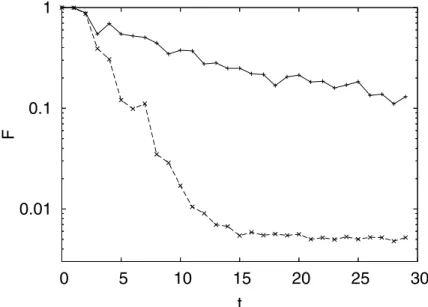
In Fig. 3 we show the corresponding curves of quantum and classical fidelity as a function of time. We note that up to the Ehrenfest time t∗, which is in this case around 3 kicks, the two quantities agree, and after that they strongly deviate. Af-tert∗one can argue that the double integral of time-correlation function (13) in formula (12) starts to behave asymptotically as ∼σt whereσ ∝ δ2 is a certain diffusion constant. This
is consistent with oscillating behavior of the Wigner function,
which is necessary in order to prevent faster - Lyapunov decay as it happens for the classical fidelity [8]. In a semi-log scale (Fig. 4) one can clearly see asymptotic exponential decays, for the quantum curve the rate is determined by Fermi Golden rule and for the classical curve by the Lyapunov exponent. The former scales with perturbation strength as∝ δ2while the
latter isδ-independent. This a clear manifestation of the qual-itativebreakdown of quantum-classical correspondence at the Ehrenfest (log-time) barriert∗. Beyondt∗quantum and clas-sical fidelities behave just in the opposite ways with respect to a degree of chaoticity of the underlying classical system.
t=2
t=3
t=5
t=10
W
ρ
W
(
ϕ,
cos
ϑ
)
ρ
(
ϕ,
cos
ϑ
)
W
·
(
W
−
W
δ)
ρ
·
(
ρ
−
ρ
δ)
t=2
t=3
t=5
t=10
FIG. 2: Zoom-in of Wigner function against classical Liouville density for chaotic dynamicsα=4. A region of the phase-space area of one Planck cell 2π(indicated above by small rectangles) is magnified in snapshots below. Again, the same representation is used as in fig. 1. Curves in Wigner function plots are nodal lines.
Loschmidt echo, namely equivalence between representations (16,22) and (17,23). Therefore, fidelity of an initial Gaussian wave-packet (coherent state) can be computed as an overlap of the initial Gaussian with the Wigner function (Liouville den-sity) after echo-dynamics. In fig. 5 we show the corresponding echoed Wigner functions and echoed Lioville densities, which again exhibit significant deviation (due to oscillatory behavior in the Wigner function) at aroundt∗.
Second, for completing the story, we make the same numer-ical experiments in the regime where the classnumer-ical dynamics is quasi-regular,α=1. Since here we have alinearinstead of an exponential divergence of classical packets, one expects the breakdown time to scale ast∗∝−1/2. In fig. 6 we show an analogous plot to fig. 1. Note that quantum Wigner func-tion and classical Liouville density for short times are here
hardly distinguishable in contrast to classically chaotic dy-namics. This fact is also illustrated by plotting in fig. 7, in comparison, quantum and classical fidelity curves for the regular case.
IV. RELATION TO DECOHERENCE MEASURES AND CONCLUSIONS
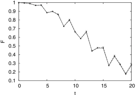
0
0.1
0.2
0.3
0.4
0.5
0.6
0.7
0.8
0.9
1
0
5
10
15
20
F
t
FIG. 3: Quantum fidelity (full curve) against classical fidelity (dashed) for classically fully chaotic dynamics,α=4. We observe clear deviation of the two curves at the log-time (or Ehrenfest time)t∗≈3.
0.01
0.1
1
0
5
10
15
20
25
30
F
t
FIG. 4: The same as in previous figure (3) but in semi-log scale. One may observe exponential decays.
In addition, there is also a link between fidelity and deco-herenceas expressed in terms of a purity of a reduced density matrix. Let us assume that we want to describe a compos-ite quantum system, which is a direct product of the central system
H
cand the environmentH
e, using a unitary quantum evolution on the product Hilbert spaceH
c×H
e. Decoherence is then directly related to the loss of purity of reduced den-sity matrixρc(t) =tre|ψ(t)ψ(t)|. The purity is quantified as I(t) =trc[ρc(t)]2and is equal to 1 for pure states and∼1/Nfor maximally mixed states, whereNis the dimension of the smaller of the Hilbert spaces
H
c, andH
e. The rate of deco-herence can thus be measured in terms of decay ofI(t)down from 1.One can show a strict inequality between purityI(t) and quantum fidelityF(t)as defined for evolving the same initial state with two dynamics: the coupled system (central system Hamiltonian plus environment Hamiltonian plus coupling) as compared to the uncoupled system (total Hamiltonian without the coupling). Namely the strong result [12] shows that
Classical
Quantum
ρ
(
ϕ,
cos
ϑ
)
zoom
W
(
ϕ,
cos
ϑ
)
zoom
t=0
t=1
t=2
t=3
t=5
t=9
FIG. 5: Wigner function and classical densities of the echo-dynamics of classically chaotic dynamics. Quantum (first column, magnified in second column) against classical (third column, magnified in fourth column). All the parameters are the same as in fig. 1.
decay drastically slower [13].
In this paper we have reviewed recent theoretical ap-proaches to describe decay of quantum fidelity in dynamical systems, and in addition provided clear phase space picture and illustration of the approach in terms of quantum Wigner functions. It is clear that seemingly paradoxical behavior of quantum fidelity with respect to the classical correspondent is a consequence of the breakdown of quantum classical corre-spondence in the Wigner function at the Ehrenfest time.
V. ACKNOWLEDGMENTS
We thank T.H.Seligman and G.Casati for useful discus-sions. The work has been financially supported by the grant P1-044 of the Ministry of Education, Science and Sports of Slovenia, and in part by the ARO grant (USA) DAAD 19-02-1-0086.
[1] R. A. Jalabert and H. M. Pastawski, Phys. Rev. Lett.86, 2490 (2001).
[2] T. Prosen, Phys. Rev. E65, 036208 (2002).
[3] Ph. Jacquod, P. G. Silvestrov, and C. W. J. Beenakker, Phys. Rev. E64, 055203 (2001).
W
(
ϕ,
cos
ϑ
)
ρ
(
ϕ,
cos
ϑ
)
W
·
(
W
−
W
δ)
ρ
·
(
ρ
−
ρ
δ)
t=0
-1 -0.5 0 0.5 1t=1
t=3
t=5
t=10
t=20
FIG. 6: Wigner function against classical density evolutions for regular dynamics. Everything is the same as in fig.1 except now forα=1.
(2002).
[5] F. M. Cucchietti, H. M. Pastawski, and D. A. Wisniacki, Phys. Rev. E65, 045206(R) (2002); S. Tomsovic and N. Cer-ruti, Phys. Rev. Lett.88, 054103 (2002); G. Benenti and G. Casati, Phys. Rev. E 66, 066205 (2002); F. M. Cucchietti et al. Phys. Rev. E 65, 046209 (2002); D. A. Wisniacki et al. Phys. Rev. E 65, 055206 (2002); D. A. Wisniacki and D. Cohen, Phys. Rev. E66, 046209 (2002); J. Emersonet al, Phys. Rev. Lett.89, 284102 (2002); G. P .Bermanet al, Phys. Rev. E66, 056206 (2002); W. G. Wang and Baowen Li, Phys. Rev. E66, 056208 (2002); T. Kottos and D. Cohen, Europhys. Lett.61, 431 (2003); D. A. Wisniacki, Phys. Rev. E67, 016205 (2003); P. G. Silvestrov, J. Tworzydlo, and C. W. J. Beenakker, Phys. Rev. E.67, 025204 (2003); and many other references.
[6] H. M. Pastawski, P. R. Levstein, and G. Usaj,
Phys. Rev. Lett.75, 4310 (1995); P. R. Levstein, G. Usaj, and H. M. Pastawski, J. Chem. Phys.108, 2718 (1998).
[7] A. Peres, Phys. Rev. A30, 1610 (1984).
[8] G. Veble and T. Prosen, Phys. Rev. Lett.92, 034101 (2004).
[9] M. Horvat and T. Prosen, J. Phys. A: Math. Gen. 36, 4015 (2003).
[10] F. Haake, M. Ku´s, and R. Schar, Z. Phys. B65, 381 (1987).
[11] G. S. Agarwal, Phys. Rev. A24, 2889 (1981).
[12] M. ˇZnidariˇc, and T. Prosen, J. Phys. A: Math. Gen.36, 2463 (2003); see also T. Prosen, T. H. Seligman, and M. ˇZnidariˇc, Phys. Rev. A67, 062108 (2003).
042105 (2004).