R ´ENYI ENTROPY AND CAUCHY-SCHWARTZ MUTUAL INFORMATION APPLIED TO MIFS-U VARIABLE SELECTION ALGORITHM: A COMPARATIVE STUDY
Leonardo Barroso Gonc¸alves
1*and Jos´e Leonardo Ribeiro Macrini
2Received June 27, 2009 / Accepted March 17, 2011
ABSTRACT.This paper approaches the algorithm of selection of variables named MIFS-U and presents an alternative method for estimating entropy and mutual information, “measures” that constitute the base of this selection algorithm. This method has, for foundation, the Cauchy-Schwartz quadratic mutual informa-tion and the R´enyi quadratic entropy, combined, in the case of continuous variables, with Parzen Window density estimation. Experiments were accomplished with public domain data, being such method com-pared with the original MIFS-U algorithm, broadly used, that adopts the Shannon entropy definition and makes use, in the case of continuous variables, of the histogram density estimator. The results show small variations between the two methods, what suggest a future investigation using a classifier, such as Neural Networks, to qualitatively evaluate these results, in the light of the final objective which is greater accuracy of classification.
Keywords: variable selection, MIFS-U, entropy, mutual information, Shannon, R´enyi, Parzen Window, Information-Theoretic Learning, ITL.
1 INTRODUCTION
Variable selection has a fundamental importance in classification systems, such as Neural Networks (Agrawal, Imielinski & Swami, 1993; Battiti, 1994; Joliffe, 1986). In this paper, the Mutual Information Variable Selector under Uniform Information Distribution (MIFS-U) is focused (Kwak & Choi, 2002). The objective of this algorithm is to select variables that are relevant for the output variable and at the same time reduce the redundancy among input vari-ables. It as the name indicates is based on concepts of Information Theory, namely, entropy and mutual information (Cover & Thomas, 2006). When the variables involved are discrete, the computation of entropy and mutual information, based on the Shannon definition, is simple
*Corresponding author
1Departamento de Engenharia El´etrica, Pontif´ıcia Universidade Cat´olica do Rio de Janeiro, Rio de Janeiro, RJ, Brasil. E-mail: [email protected]
and direct, since the joint and marginal distributions can be estimated simply by counting the samples. However, when at least one of the variables in question is continuous, the computation that involves integration becomes difficult due to the limited number of samples. A solution is usually to insert the discretization of the data as a step of pre-processing, and to estimate the unknown density by the histogram. Not always, however, the discretization is made clearly and adequately. This paper shows a alternative method based on the Cauchy-Schwartz quadratic mutual information and the R´enyi quadratic entropy, this combined with the Parzen Window density estimator (Silverman, 1986), and in this way the computations become direct without need of a pre-processing step. Initially, this paper shows a introduction to information theory based on the Shannon and the R´enyi entropies and additionally shows the Cauchy-Schwartz mutual information, concept used in Information-Theoretic Learning (ITL) (Pr´ıncipe, 2000; Pr´ıncipe, Fisher & Xu, 1998). Next, the MIFS-U variable selector and the estimation methods of entropy and mutual information are shown. Finally, both methods are applied in datasets and the results are compared in order to obtain an initial notion of the performance of the proposed method.
2 INFORMATION THEORY
Information theory was developed by Shannon in communication engineering applications in the early 1940s. This theory, due to its innovative character and mathematical elegance, had great impact not only in engineering but also in several areas such as statistics and economy.
This section summarizes, in a descriptive way, theoretical foundations of information theory. For demonstrations and explanations on the subject matter, see, in particular, reference Cover & Thomas (2006).
2.1 Shannon Entropy and Shannon Mutual Information
The uncertainty characterizes the information gain that the occurrence of an event can cause. Therefore, such uncertainty can be translated into the probability of occurrence of its event. An event whose occurrence is right doesn’t bring any increment of information, because the whole information is already contained in its occurrence certainty. In this way, it can be said that the determination of the amount of information produced by the occurrence of an event is determined by the amount of “surprise” that such occurrence brings.
The entropy in information theory corresponds therefore to the probabilistic uncertainty associ-ated with a probability distribution.
Definition 1– TheShannon entropy H(X)of a discrete random variable X, with a probability mass function fx(x),x∈X (the domain set of the variable), is defined by
H(X)= −X x∈X
fx(x)log fx(x) (1)
It results from the own definition thatH(X)≥0. It is commom to denote the above quantity by
Definition 2– The(Shannon) joint entropy H(X,Y)of a pair of discrete random variables(X,Y) with a joint probability distribution fx yis defined as
H(X,Y)= −X x∈X
X
y∈Y
fx y(x,y)logfx y(x,y) (2)
Definition 3– The(Shannon) conditional entropy H(Y|X)(that is, ofY given the knowledge of
X)is defined as
H(Y|X)= −X x∈X
X
y∈Y
fx y(x,y)log fy|x(y|x) (3)
Definition 4– TheKullback-Leibler relative entropy(or,(asymmetrical) divergence) between two probability mass functions f andgis defined as
DK L(fkg)=X x∈X
f(x)log f(x)
g(x) =Ef
log f(x)
g(x)
(4)
DK L(fkg)≥0 with equality if and only if f(x)=g(x), for everyx∈X.
The Kullback-Leibler relative entropy (or, divergence) is a similarity measure between strictly positive functions, it is also referred as “distance” between distributions, however, it is not a true distance since it is not symmetric and does not satisfy the triangle inequality. It is very used in the comparison between two functions. In that case, the functiong represents the reference function. The Kullback-Leibler divergence is intimately related with the Shannon entropy.
Definition 5– The(Shannon) mutual information I(X;Y)between two discrete random vari-ablesX andY, with a joint probability mass function fx y(x,y)and marginal probability mass functions fx(x)and fy(y)is given by the relative entropy between the joint distribution and the
product of the marginal distributions:
I(X;Y)=X x∈X
X
y∈Y
fx y(x,y)log
fx y(x,y)
fx(x)fy(y)
=DK L(fx y(x,y)kfx(x)fy(y))≥0 (5)
with equality if and only if fx y(x,y)= fx(x)fy(y)(that is, ifX andY are independent).
Starting from Eq. (5), it can be said that the mutual information is a measure of statistical inde-pendence. The higher the mutual information, the stronger the association between the variables.
Next, the concept of differential entropy is introduced that it is the entropy of a continuous random variable. The differential entropy is similar in many forms to the entropy of a discrete random variable, but there are important differences, and it is therefore necessary to pay attention to the usage of that concept. Note that unlike the discrete case, the differential entropy can be negative but, as it will be seen, the differential version of the mutual information will always be non-negative.
Definition 6– TheShannon differential entropy h(X)of a continuous random variableX, with a probability density function fx(x),x ∈X (the support set of the variable), is defined by
h(X)= − Z
X
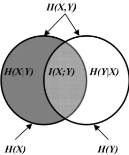
Figure 1– The relation between the entropy and the mutual information.
Definition 7– The(Shannon) joint differential entropy h(X,Y)of a pair of continuous random variables(X,Y), with joint density fx y, is defined as
h(X,Y)= − Z
Y
Z
X
fx y(x,y)log fx y(x,y)d x d y (7)
Definition 8– The(Shannon) conditional differential entropy h(X|Y)is defined as
h(X|Y)= − Z
Y
Z
X
fx y(x,y)logfx|y(x|y)d x d y (8)
Definition 9– TheKullback-Leibler relative entropy (or,(asymmetrical) divergence) between two densities f andgis defined as
DK L(fkg)= Z
X
f(x)log f(x)
g(x)d x =Ef
log f(x)
g(x)
(9)
DK L(fkg)≥0 with equality if and only if f =g almost everywhere.
Definition 10– The (Shannon) mutual information I(X;Y)between two continuous random variablesXandY, with joint density fX Y and marginal densities fXand fY is defined by
I(X;Y)= Z
Y
Z
X
f(x,y)log fx y(x,y)
fx(x)fy(y)
d x d y=DK L(fx y(x,y)kfx(x)fy(y))≥0 (10)
Although, unlike the entropy for discrete random variables, the differential entropy cannot be interpreted as a randomness (or uncertainty) measure, the mutual information has the same interpretation as in the discrete case.
2.2 R´enyi Entropy and R´enyi Mutual Information
Definition 11– The orderα R´enyi entropy HRα(X)of a discrete random variable X, with a
probability mass function fx(x),x∈X, is defined as
HRα(X)= 1
1−αlog
X
x∈X
The Shannon entropy appears as a special case of the R´enyi entropy by taking the limit of it as α→1.
Of particular interest is R´enyi’s entropy of order two, which is called theR´enyi quadratic entropy.
Definition 12– Theorderαdifferential R´enyi entropy hRα(X)of a continuous random variable
X, with a probability density function fx(x), is defined as
hRα(X)=
1 1−αlog
Z
X
fxα(x)d x
(12)
Again, of particular interest is whenα=2, and it is denoteddifferential R´enyi quadratic entropy.
Definition 13– TheR´enyi relative entropy(or,(asymmetrical) divergence)of orderαbetween two probability mass functions f andgis defined as
DRα(fkg)=
1 α−1log
X
x∈X
g(x)
f(x)
g(x)
α = 1
α−1log X
x∈X
fα(x)g1−α(x),
for α >0 and α6=1
(13)
DRα(fkg) ≥ 0 with equality if and only if f(x) = g(x), for every x ∈ X. Note that the
Kullback-Leibler divergence is obtained in the limit asα→1.
Definition 14– TheR´enyi relative entropy(or,(asymmetrical) divergence)of orderαbetween two densities f andg(Neemuchwala, 2005) is defined as
DRα(fkg)=
1 α−1log
Z
X
g(x)
f(x) g(x)
α
d x= 1
α−1log Z
X
fα(x)g1−α(x)d x,
for α >0 and α6=1
(14)
DRα(fkg)≥0 with equality if and only if f =g almost everywhere.
The R´enyi divergence may also be used as a measure of mutual information between random variables, by considering the divergence between the joint distribution and the product of marginal distributions, according to the following definitions which are based only on the quad-ratic divergence (of order 2), being simply represented byIR(X;Y).
Definition 15– TheR´enyi mutual information IR(X;Y)between two discrete random variables X andY, with a joint probability mass function fx y(x,y)and marginal probability mass func-tions fx(x)and fy(y)is given by the relative entropy between the joint distribution and the
product of the marginal distributions:
IR(X;Y)=logX
x∈X
X
y∈Y
fx y2(x,y)
fx(x)fy(y)=DR2(fx y(x,y)kfx(x)fy(y))≥0 (15)
Definition 16– TheR´enyi mutual information IR(X;Y)between two continuous random vari-ables X andY, with joint density fx y(x,y)and marginal densities fx(x)and fy(y)is defined by
IR(X;Y)=log Z
Y
Z
X
fx y2(x,y)
fx(x)fy(y)
d x d y=DR2(fx y(x,y)kfx(x)fy(y))≥0 (16)
with equality if and only if fx y = fxfyalmost everywhere(that is, ifXandY are independent).
The R´enyi mutual information, unlike the Shannon mutual information, can not be expressed in terms of R´enyi entropies (Jenssen, 2005). However, the Cauchy-Schwartz mutual information, which is introduced in the next section, can be expressed, as will be seen, by R´enyi quadratic entropy.
2.3 Cauchy-Schwartz Mutual Information
Principeet al.(2000) defined a measure of divergence between probability density functions (or probability mass functions) based on the Cauchy-Schwartz inequality between vectors.
Definition 17 – The Cauchy-Schwartz (simetrical) divergence between two probability mass functions f(x)andg(x)is defined by
DC S(fkg)= −log
P
x∈X
f(x)g(x)
s P
x∈X
f2(x) P x∈X
g2(x)
(17)
DC S(fkg)≥0 with equality if and only if f(x)=g(x), for everyx∈X.
Developing the previous equation, one gets
DC S(fkg)= −logX
x∈X
f(x)g(x)−1
2 −log X
x∈X
f2(x)
! −1
2 −log X
x∈X
g2(x)
! (18)
Expressing the second member of Eq. (18) through the R´enyi entropy, the following is obtained:
DC S(fkg)=hR2(f ×g)− 1
2hR2(f)− 1
2hR2(g) (19)
where
• hR2(f)is the R´enyi quadratic entropy with respect to f.
• hR2(g)is the R´enyi quadratic entropy with respect tog.
• hR2(f ×g)can be interpreted as thecross-entropybetween f andg.
Definition 18– TheCauchy-Schwartz (simetrical) divergencebetween two densities f andgis defined by
DC S(fkg) = −log
R
X f(x)g(x)d x
q R
X f2(x)d x
R
Xg2(x)d x
DC S(fkg)≥0, with equality if and only if f =g almost everywhere, and the integrals involved are all quadratic forms of probability density functions.
In a similar way, Eq. (19) is also obtained by developing the previous equation.
Definition 19 – The Cauchy-Schwartz mutual information IC S(X;Y) between two discrete random variablesX andY, with a joint probability mass function fx y(x,y)and marginal
prob-ability mass functions fx(x)and fy(y)is given by the divergence between the joint distribution and the product of the marginal distributions:
IC S(X;Y)=hR2(fX Y× fXfY)− 1
2hR2(fX Y)− 1
2hR2(fXfY)=DC S(fx ykfxfy)≥0 (21) with equality if and only if fx y(x,y)= fx(x)fy(y)(that is, ifX andY are independent).
Definition 20– TheCauchy-Schwartz mutual information IC S(X;Y)between two continuous random variablesX andY, with joint density fx y(x,y)and marginal densities fx(x)and fy(y)
is given by Eq. (21), with equality if and only if fx y = fxfy almost everywhere(that is, if X
andY are independent).
3 MUTUAL INFORMATION VARIABLE SELECTION UNDER UNIFORM
INFORMATION DISTRIBUTION (MIFS-U)
Input variable selection plays an important role in classifying systems such as neural networks (NNs). A input variable can be classified as relevant, irrelevant or redundant and from the view-point of managing a dataset which can be huge, reducing the number of variables by selecting only the relevant ones is desirable. In doing so, higher performances with lower computational effort is expected (Kwak & Choi, 2002).
Hosmer & Lemeshow (1989) highlight the importance of variable selection, because with a smaller number of variables, the model tends to be more generalizable and robust.
Problems of variable selection has been tackled by several researchers such as Battiti (1994), Joliffe (1986) and Agrawalet al.(1993). One of the most popular methods for dealing with this problem is the principal component analysis (PCA) method (Joliffe, 1986). However, when the maintenance of the original variables is wanted, this method is not adequate.
The algorithm approached in this paper, that is the MIFS-U – Mutual Information Feature (Vari-able) Selector under Uniform Information Distribution – was presented by Kwak & Choi (2002), with the objective of overcoming the limitation of variable selector proposed by Battiti (1994), producing better performance of the variable selection procedure. Such algorithm can be used in any classifying systems for its simplicity whatever the learning algorithm may be. But the performance can be degraded as a result of errors in estimating the mutual information.
3.1 The FRn-k Problem and the Ideal Selection Algorithm
select-ing the most relevantkvariables from a set ofnvariables and Battiti (1994) named it as “feature reduction – FR” problem. Such process is described as follows:
[FRn – k]: Given an initial set of n variables, find the subset withk<n variables that is “max-imally informative” about the class (output variable). The problem of selecting input variables can be solved by computing the mutual information (MI) between input variables and output classes. If the mutual information between input variables and output classes could be exactly obtained, the FRn – k problem could be reformulated as follows:
[FRn – k]: Given an initial set F withn variables and the output variable D, find the subset
S ⊂F withkvariables that minimizesH(D|S), that is, that maximizes the mutual information
I(D;S). The selection method here adopted is known as “greedy selection”. In this method, from the empty set of selected variables, the best input variable of the current state is added one by one. Thisideal selection algorithmusing mutual information is realized as follows:
1) (Initialization) setF ←“initial set ofnvariables”,S←“empty set.”
2) (Computation of the MI with the output class),∀φi ∈ F, computeI(D;φi).
3) (Selection of the first variable) find the variable that maximizes I(D;φi), set F ← F\ {φi},S ← {φi}.
4) (Greedy selection) repeat until desired number of variables are selected:
a) (Computation of the joint MI between variables),∀φi ∈ F, computeI(D;φi,S).
b) (Selection of the next variable) choose the variableφi ∈ F that maximizes I(D;
φi,S), and setF ←F\{φi},S← {φi}.
5) Output the setScontaining the selected variables.
In practice, the realization of this algorithm is unviable due to the high dimensionality of the vector of variables in the computation of I(D;φi,S), since the objective is to select k(k < n)variables, and therefore the vector S (composed of the variables already selected), reaches dimension(k−1).
3.2 The MIFS-U Variable Selector
The ideal algorithm (Battiti, 1994) tries to maximize I(D;φi, φs)(area II, III and IV in Fig. 2)
and, according to Kwak & Choi (2002), this can be rewritten as
I(D;φi, φs)=I(D;φs)+I(D;φi|φs) , (22)
where I(D;φi|φs)represents the remaining mutual information between the output class Dand
the variableφi for a givenφs. This is shown as area III in Figure 2, whereas the area II plus
area IV represents I(D;φs). Since I(D;φs)is common for all the candidate variables to be
to find the variable that maximizes I(D;φi|φs)(area III). However, calculating I(D;φi|φs)
requires as much work as calculatingI(D;φi;φs). SoI(D;φi|φs)is approximately computed
with I(φi;φs)and I(D;φi), which are relatively easy to calculate. The conditional mutual
information can be represented as
I(D;φi|φs)=I(D;φi)− {I(φi;φs)−I(φi;φs|D)} (23)
where I(φi;φs)corresponds to arera I and IV, and I(φi;φs|D)corresponds to area I. So the
term I(φi;φs)−I(φi;φs|D)corresponds to area IV. The term I(φi;φs|D)means the mutual
information between the already selected variableφs and the candidate variableφi for a given
classD.
If conditioning by the classDdoes not change the ratio of the entropy ofφsand the mutual
infor-mation betweenφi andφs, that is, if the following relations holds (condition of the algorithm):
H(φs|D) H(φs)
= I(φi;φs|D) I(φi;φs)
(24)
I(φi;φs|D)can be represented as
I(φi;φS|D)=
H(φs|D) H(φs)
I(φi;φs) (25)
Using the equation above and Eq. (23), the following is obtained:
I(D;φi|φs)=I(D;φi)−
I(D;φs) H(φs)
I(φi;φs). (26)
Assuming that each region in Figure 2 corresponds to its corresponding information, the condi-tion presented in Eq. (24) is hard to satisfied when informacondi-tion is concentrated on one of the following regions: H(φs|φi;D),I(φs;φi|D),I(D;φs|φi)or I(D;φs;φi). It is more likely that
condition (24) hods when information is distributed uniformly throughout the region of H(φs)
in Figure 2. Because of this, the algorithm is simply called the MIFS-U algorithm.
Then the revised step 4 of the ideal selection algorithm takes the following form:
4) (Greedy selection) repeat until desired number of variables are selected:
a) (Computation of entropy)∀φs ∈S, computeH(φs), if is not already available.
b) (Computation of the MI between variables), for all couples of variables(φi, φs)with
φi ∈F andφs ∈ S, computeI(φi;φs), if it is not yet available.
c) (Selection of the next variable) choose a variableφi ∈ Fthat maximizesI(D;φi)−
βP
φs∈S(I(D;φs)/H(φs)) I(φi;φs)and setF ←F\ {φi},S← {φi}.
φ φ
φ
φ
φ
φ
Figure 2– The relation between input variables and output classes.
the mutual information with the output. Asβgrows aumenta, it excludes the redundant variables more efficiently. In generalβ can be taken as 1 (Breimanet al., 1984). In this case there is a balance in terms of weight between the redundancy of the candidate variable and the mutual information between this variable and the output. So, for all the experiments in this paper,β =1 is adopted.
Kwak & Choi (2002) point out that the MIFS-U algorithm can be applied to large problems without excessive computational efforts.
4 ESTIMATION METHODS OF ENTROPY AND MUTUAL INFORMATION
without need of a pre-processing step. From now on this method will be called Cauchy-Schwartz/Parzen-Rosenblatt Method.
4.1 Shannon/Histogram Method
In the case of continuous variables, to avoid adopting a parametric model for the unknown den-sity, a common solution is to apply non-parametric density estimation methods. The oldest and the most widely used density estimator is the histogram (Silverman, 1986). In this paper, the rel-ative frequency histogram is actually used, not the density histogram, where the only difference is that the latter is normalized to integrate to 1 (Scott, 1992).
As all the continuous variables are normalized in the interval [−1,1], the interval is simply divided into 20 subintervals of equal width(h =0,1). Each subinterval is interpreted as a class and each computed relative frequency is taken as a probability. In other words, a discretization – a continuous variable becomes discrete – is done. Then there are no more obstacle to the necessary computations, and the Shannon entropy definition, widely used in the literature, can be easily applied.
In order to maintain a harmonic nomenclature, a specific class of a discretized continuous vari-able or a (distinct) value of a discrete varivari-able will simply be represented byx(and the set of such values or classes will be represented by X), and therefore, this distinction is no longer needed.
So the following can be written:
ˆ
fx(x)= 1 n
n X
i=1
ξ(xi,x) ,∀x∈X. (27)
whereξx(xi)is the Indicator Function, that is,
ξ(xi,x)= (
1 , if xi ∈x(class)
0 , otherwise (Discretized Continuous Variable)
or
ξ(xi,x)= (
1 , if xi =x(value)
0 , otherwise (Discrete Variable)
and the joint distribution of two (discrete or discretized continuous) variables is the following:
ˆ
fx y(x,y)= 1 n
n X
i=1
ξx(xi)ξy(yi) ,∀x∈X,∀y∈Y. (28)
Therefore, considering the discretization of continuous variables as a step of pre-processing of the data, the necessary computations for the MIFS-U algorithm are merely the following ones:
• Entropy of a discrete variable (EntD),
EntD – Shannon Entropy of a discrete variable
ˆ
H(X)= −X x∈X
ˆ
fx(x)log fxˆ(x) (29)
MI-DD – (Shannon) Mutual Information between two discrete variables
ˆ
I(X;Y)=X x∈X
X
y∈Y
ˆ
fx y(x,y)log fx yˆ (x,y)
ˆ
fx(x)fyˆ(y) (30)
4.2 Cauchy-Schwartz/Parzen-Rosenblatt Method
In the context of variable selection in nonlinear systems, the estimation of the mutual informa-tion between variables directly from the data, where at least one of them is continuous, without hypotheses about theprioridistribution of the data, has vital practical importance. This can be reached using the Cauchy-Schwartz divergence, which is a substitute of the Kullback-Leibler divergence, integrated with the Parzen Window estimator.
The Kullback-Leibler divergence, based on the Shannon entropy, is, in its simplicity, an usual measure of mutual information between two random variables. However, neither this nor the equivalent for the R´enyi entropy can be integrated with the Parzen Window estimator (Pr´ıncipe et al., 1998). Xuet al.(1998) presented a method that combines the Cauchy-Schwartz Divergence with Parzen Windowing for estimating the mutual information directly from the data.
4.2.1 Parzen Window Density Estimator
According to Scott (1992), given a set of samples of fx{x1,x2, . . . ,xn}, the Kernel Density Estimator – or the Parzen Window Estimator – may be written compactly as
ˆ
fx(x)= 1 n
n X
i=1
K(x−xi,h) (31)
whereh=h(n) >0 is the window width or smoothing parameter.
So fxˆ(x)can be seen as an “average of curves” centered at the samples.
The Kernel FunctionK(∙)is usually non-negative and with unitary integral, that is, a probability density function (Silverman, 1986). Furthermore, often K(∙)is chosen to be a symmetric and unimodal density.
For the later use in this paper, the Gaussian Kernel Function will be considered, defined below.
G(w, φ)=(2π φ)−12 exp −ω 2
2φ
!
(32)
The choice of the window width affects the density estimate much more than the choice of the Kernel Function (Scott, 1992). So the choice of the Kernel Function is not crucially impor-tant. However, the Gaussian Function has a property that will be extremely advantageous in the context of this paper.
There exist several methods for selecting the window widthh, each having its properties (Wand & Jones, 1995). The method here used is known as “Normal Reference Rule”, and the window width is given by
hot =1,06σn−1/5 (33)
The standard deviationσ can be estimated, starting from the data, by the sample standard devi-ationsor by a robust measure like the interquartile range. In this paper, a commitment solution between both estimators is used, similar to the form presented by Silverman (1986):
ˆ
hot=0,9 min(s,Iqˆ )n−1/5 (34)
In the bivariate case, using a single window width for both variables and taking the same consid-erations in regard to the estimation of the standard deviation in the univariate case, the following is adopted in this paper:
hot ≈0,85 min
s12+s22
2 !−12
,
ˆ
Iq(1)+ ˆIq(2)
2
n− 1
6 (35)
4.2.2 Necessary Computations for the MIFS-U Algorithm
The types of computation required for the MIFS-U algorithm are presented below, using indis-tinctly the notationhR2in the representation the R´enyi entropy, whether differential or not.
EntD – R´enyi Entropy of a discrete variable
ˆ
hR2(X)= −log X
x∈X
ˆ
fx2(x) (36)
EntC – R´enyi Entropy of a continuous variable
Estimating the density through the Gaussian Kernel Function
ˆ
fx(x)= 1 n
n X
i=1
G(x−xi, σ2)
!
(37)
and applying the property of the integration of the product of Gaussian kernels, shown below,
Z
G x−ai, σ12G x−aj, σ22
d x=G ai−aj, σ12+σ22
the R´enyi quadratic entropy is easily estimated by
ˆ
hR2(X) = −log 1 n2 n X
i=1
n X
j=1
G xi−xj,2σ2
(39)
Thus, the R´enyi quadratic entropy can be estimated as a sum of local interactions, as defined by the kernel, over all pairs of samples.
MI-DD – (Cauchy-Schwartz) Mutual Information between two discrete variables
IC S(X;Y)=hR2(fX Y × fXfY)− 1
2hR2(fX Y)− 1
2hR2(fXfY) (40)
where
ˆ
hR2(fx yˆ × ˆfxfyˆ) = −log X
Y
X
X
ˆ
fx y(x,y)fxˆ(x)fyˆ(y) (41)
ˆ
hR2(fx yˆ )= −log X
Y
X
X
ˆ
fx y2(x,y) (42)
ˆ
hR2(fxˆ fyˆ)= −log X
Y
X
X
ˆ
fx2(x)fˆy2(y) (43)
MI-CC – (Cauchy-Schwartz) Mutual Information between two continuous variables
As seen, the entropy of a single variable is easily evaluated as interactions between pairs of samples. This concept will now be extended to mutual information between variables. Thus, in the continuous case, Eq. (40) is the second member of the equation given by
ˆ
hR2(fx yˆ × ˆfxfyˆ)= −log Z
Y
Z
X
ˆ
fx y(x,y)fxˆ(x)fyˆ(y)d x d y
= −log 1 n3 n X
i=1
n X
j=1
G(xi−xj,2σ2)
n X
l=1
G(yi−yl,2σ2)
! (44) ˆ
hR2(fx yˆ )= −log Z
Y
Z
X
ˆ
fx y2(x,y)d x d y
= −log 1 n2 n X
i=1
n X
j=1
G(xi−xj,2σ2)G(yi−yj,2σ2)
(45)
ˆ
hR2(fxˆ fˆy)= −log Z
Y
Z
X
ˆ
fx2(x)fˆy2(y)d x d y
= −log 1 n4 n X
i=1
n X
j=1
G(xi−xj,2σ2)
" n
X
k=1
n X
l=1
G(yk−yl,2σ2)
#
MI-DC – (Cauchy-Schwartz) Mutual Information between a discrete variable(Y)and a contin-uous variable(X)
Consider the following definitions:
v=number of distinct values ofY in the sample.
yp=pth distinct value ofY in the sample.
np=number of samples ofXrelated to the valueypofY.
Here two different notations are used for the samples of X. A sample is written with a single subscript xi(1 ≤ i ≤ n)when the identification of the Y-value related to it is irrelevant. If it is relevant, xps indicates the sample of X, with index 1 ≤ s ≤ np, related to the value yp
(1≤ p≤v)ofY.
ˆ fy(yp)=
np n
v
X
p=1
np=n (47)
Estimating the densities through the Gaussian Kernel Function, in the case of the continuous vari-able, and using the property of the integration of the product of Gaussian kernels, the entropies appearing in Eq. (40) are estimated by
ˆ
hR2(fx yˆ × ˆfxfyˆ)= −log
v
X
p=1
Z
X
ˆ
fx y(x,yp)fxˆ(x)fyˆ(yp)d x
= −log 1
n3 v
X
p=1
" np
np
X
s=1
n X
i=1
G xps −xi,2σ2
# (48)
ˆ
hR2(fx yˆ )= −log
v
X
p=1
Z
Y
ˆ
fx y2(xi,y)d y= −log 1
n2 v
X
p=1
np
X
s=1
np
X
t=1
G xps−xpt,2σ2 (49)
ˆ
hR2(fxˆ fˆy)= −log
v
X
p=1
Z
X
ˆ
fx2(x)fˆy2(yp)d x
= −log 1 n4 v X
p=1
n2p n X
i=1
n X
j=1
G xi −xj,2σ2 (50) 5 EXPERIMENTS
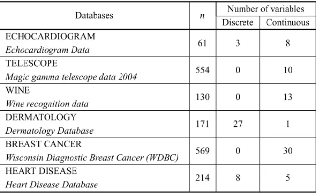
5.1 A Brief Description of the Databases
The databases were extracted from theUCI Machine Learning Repository
It is not in the scope of this study a specific analysis of the databases, since the use of the databases considered here has in view the mere comparison of the results regarding the selection order by the MIFS-U algorithm, considering the two estimation methods of entropy and mutual information presented in this paper.
In the subsequent table, it can be observed the following information:
• the number of complete samples considered in each database(n),
• the number of discrete and continuous variables (ignoring the output).
Table 1– Databases.
Databases n Number of variables
Discrete Continuous ECHOCARDIOGRAM
Echocardiogram Data 61 3 8
TELESCOPE
Magic gamma telescope data 2004 554 0 10
WINE
Wine recognition data 130 0 13
DERMATOLOGY
Dermatology Database 171 27 1
BREAST CANCER
Wisconsin Diagnostic Breast Cancer (WDBC) 569 0 30
HEART DISEASE
Heart Disease Database 214 8 5
5.2 Comparison of the Methods
The comparison of the results of the selection by the MIFS-U, regarding both estimation methods of entropy and mutual information presented in this paper, is shown in following tables. The val-ues are normalized to 1. The analysis focuses the first five selected variables. For simplification, the Shannon/Histogram and Cauchy-Schwartz/Parzen-Rosenblatt Methods will be respectively designated by the acronym SH and CSPR. It is worth to emphasize that the comments are based on the simple observation. For a more detailed analysis, it would be necessary the application of a classifier in order to investigate the accuracy of classification regarding both groups of selected variables by the MIFS-U.
would have little influence on the result (that is, the classification) that must be ascertained by application of a classifier.
Table 2– Comparative result of the selection by the MIFS-U – ECHOCARDIOGRAM. ECHOCARDIOGRAM Database
Order SH Method CSPR Method Var. MI with Output Var. MI with Output
1st 4 1.0000 4 1.0000
2nd 1 0.7424 1 0.8705
3rd 2 0.0275 10 0.2123
4th 3 0.0258 5 0.1324
5th 10 0.2963 9 0.1246
Table 3– Comparative result of the selection by the MIFS-U – TELESCOPE. Database TELESCOPE
Order SH Method CSPR Method Var. MI with Output Var. MI with Output
1st 1 1.0000 9 1.0000
2nd 9 1.0000 2 0.1874
3rd 8 0.9963 1 0.1441
4th 10 1.0000 7 0.1029
5th 6 0.9963 3 0.0661
Regarding the TELESCOPE database (Table 3), the selection made by the MIFS-U using the two methods is again practically the same in relation to the first three variables selected by the algorithm. Equally, the possibility exists that the remaining variables in the two sets of selected variables have similar contibution for the output, but this must be checked by application of a classifier. It is noteworthy that, using the SH method, the mutual information of each selected variable with respect to the output is practically the same, which does not happen using the CSPR method, reflecting a more discriminating power.
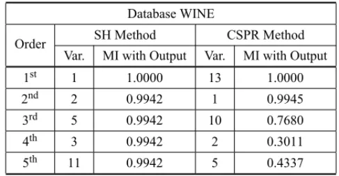
Table 4– Comparative result of the selection by the MIFS-U – WINE. Database WINE
Order SH Method CSPR Method Var. MI with Output Var. MI with Output 1st 1 1.0000 13 1.0000
2nd 2 0.9942 1 0.9945
3rd 5 0.9942 10 0.7680
4th 3 0.9942 2 0.3011
5th 11 0.9942 5 0.4337
Table 5– Comparative result of the selection by the MIFS-U – DERMATOLOGY. Database DERMATOLOGY
Order SH Method CSPR Method Var. MI with Output Var. MI with Output 1st 16 1.0000 16 1.0000 2nd 23 0.9820 18 0.9703 3rd 28 0.4910 17 0.8514 4th 27 0.0048 20 0.5053 5th 22 0.0048 7 0.6242
Regarding the DERMATOLOGY database (Table 5), the variable 16 was the first variable se-lected by the MIFS-U using both methods. However the variable 23, second variable sese-lected by the algorithm using the SH method, is one of the last ones classified using the CSPR method. The inverse happens with the variable 18. Although the mutual information of each one of these variables with respect to the output is significant, the possibility exists that these variables are redundant, what must be examined in more detail. For both methods, the mutual information between them is considerable, that is, 0,852(SH) and 0,771(CSPR).
Regarding the BREAST CANCER database (Table 6), the variables 23 and 28, although in in-verted order, were the first variables selected by the MIFS-U using both methods. It can be still observed that the other three variables, in relation to both methods, except the variable 14 in the SH case, have very low mutual information with the output, indicating probably a particular contribution of these variables.
Table 6– Comparative Result of the Selection by the MIFS-U – BREAST CANCER. Database BREAST CANCER
Order SH Method CSPR Method Var. MI with Output Var. MI with Output 1st 23 1.0000 28 1.0000 2nd 28 0.9520 23 0.8659 3rd 14 0.6463 20 0.0843 4th 17 0.2722 12 0.0268 5th 2 0.2969 29 0.1648
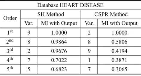
Table 7– Comparative Result of the Selection by the MIFS-U – HEART DISEASE. Database HEART DISEASE
Order SH Method CSPR Method Var. MI with Output Var. MI with Output
1st 9 1.0000 2 1.0000
2nd 8 0.9864 8 0.5806
3rd 2 0.9676 9 0.4194
4th 7 0.7022 1 0.3871
5th 5 0.6823 7 0.3065
6 FINAL REMARKS
about the unknown density – in almost all real world problems, the only information available is contained in the data collected. It should be always kept in mind that the process of variables selection must be as accurate as possible, but without losing its simplicity. In practice, simplicity becomes a paramount consideration. If such process involves complex techniques, it ends up becoming a problem in itself, rather than being a facilitator for a later stage of classification, through, for example, learning of an Artificial Neural Network (ANN).
Experiments were conducted, comparing the Cauchy-Schwartz / Parzen-Rosenblatt method (CSPR), presented in this paper, with the Shannon/Histogram method (SH), widely used, based on the Shannon entropy definition and that uses the discretization of continuous variables as a step of pre-processing of the data. The results, focusing on the set of the first five selected variables, were similar. As the comparison was purely speculative, a more careful analysis must be realized by applying a classifier (or more than one), so that the methods can be compared through the effective performance of the sets of selected variables by the MIFS-U algorithm. Besides, it is strongly recommended the participation of a professional in the field of knowledge concerning the databases covered in this paper, as it would certainly allow a better evaluation of the methods. Lastly, the CSPR method works directly with the data, providing, theoretically, greater accuracy. On the other hand, the SH method – that uses the discretization, which in principle could mask some relevant “information” from the data – is simpler, which explains its widespread use.
REFERENCES
[1] AGRAWALR, IMIELINSKI T & SWAMIA. 1993. Database minimng: A performance perspective.
IEEE Trans. Knowledge Data Eng.,5: December 1993.
[2] BATTITIR. 1994. Using mutual information for selecting features in supervised Neural net learning.
IEEE Trans. Neural Networks,5: 537–550.
[3] BREIMANLET AL. 1984.Classification and Regression Trees. Wadsworth, Belmont, CA.
[4] CAVALCANTE CC. 2001. Predic¸˜ao Neural e Estimac¸˜ao de Func¸˜ao Densidade de Probabilidades Aplicadas `a Equalizac¸˜ao Cega. Dissertac¸˜ao de Mestrado, DEE/UFC.
[5] COVERTM & THOMASJA. 2006.Elements of information theory. 2nded., Jonh Wiley & Sons, Inc., Hoboken, New Jersey.
[6] DUDARO & HARTPE. 1973.Pattern Classification and Scene Analysis. Jonh Wiley & Sons, Inc., New York.
[7] HARTLEYRV. 1928 Transmission of Information.Bell System Technical Journal,7: 535–563, July 1928.
[8] JOLIFFEIT. 1986.Principal Component Analysis. Springer-Verlag, New York.
[9] KULLBACKS. 1968.Information Theory and Statistics. Dover Publications, Inc., New York. [10] KWAKN & CHOIC. 2002. Input Feature Selection for Classification Problems.IEEE Trans. Neural
[11] MACRINIJLR. 2004. Estimac¸˜ao do Risco de Recidiva em Crianc¸as Portadoras de Leucemia Lin-fobl´astica Aguda Usando Redes Neurais. Tese de Doutorado, DEE/PUC-Rio.
[12] NEEMUCHWALAHF. 2005. Entropic Graphs for Image Registration. PhD thesis, University of Michi-gan.
[13] PRINCIPEJCET AL. 2000. Learning from examples with information theoretic criteria.Journal of VLSI Signal Proc. Systems,26(1/2): 61–77, August 2000.
[14] PRINCIPEJC, FISHERIII JW & XUDX. (1998).Information-Theoretic Learning. University of Florida, Gainesville.
[15] RODRIGUESTB. 2006. Selec¸˜ao de Vari´aveis e Classificac¸˜ao de Padr˜oes Utilizando Redes Neurais com Aplicac¸˜ao no Diagn´ostico de Doenc¸a Card´ıaca. Dissertac¸˜ao de Mestrado, DEE/PUC-Rio. [16] SCOTTDW. 1992.Multivariate Density Estimation.Jonh Wiley & Sons, Inc., New York.
[17] SHANNONCE & WEAVER W. 1949The Mathematical Theory of Communication. Univ. Illinois Press, Urbana, IL.
[18] SILVEIRAGB. 1992.Estimac¸˜ao de Densidades e de Func¸˜oes de Regress˜ao. UFRJ, Rio de Janeiro. [19] SILVERMAN BW. 1986.Density Estimation for Statistics and Data Analysis. Chapman and Hall,
London.
[20] VIOLAP & WELLSIII WM. 1997. Alignment by Maximization of Mutual Information. Interna-tional Journal of Computer Vision,24(2): 137–154.
[21] WANDMP & JONESMC. 1995.Kernel Smoothing. Chapman and Hall, London.
[22] XUD. 1999. Energy, Entropy and Information Potential for Neural Computation. PhD thesis, Uni-versity of Florida.