Umbilic and Tangential Singularities on Configurations of Principal Curvature Lines

www.scielo.br/aabc

Umbilic and Tangential Singularities on Configurations of Principal Curvature Lines

RONALDO GARCIA1 and JORGE SOTOMAYOR2

1_{Instituto de Matemática e Estatística – Universidade Federal de Goiás, Cx. Postal 131} 74001-970 Goiânia, GO, Brazil

2_{Instituto de Matemática e Estatística, Universidade de São Paulo, Cidade Universitária} 05508-900 São Paulo, SP, Brazil

Manuscript received on June 20, 2001; accepted for publication on October 18, 2001; contributed byJorge Sotomayor

ABSTRACT

In this paper is studied the relationship between quadratic tangencies of principal lines with the boundary of a surface and the Darbouxian umbilics of a smooth boundaryless surface which approximates it through the process of thickening and smoothing defined here.

Key words:tangential singularity, umbilic point, principal configuration.

1 INTRODUCTION

Consider a smooth i.e. C∞, compact, connected, oriented and regular surfaceSwith boundaryB embedded intoR3. Without loss of generality, we can assume that_Sis contained in a boundaryless

surface_Sˆ _{defined implicitly by a smooth functionf:}R3→Rsuch that

ˆ

S= {p∈R3:f =0}

and thatSandBare given in terms of a smooth functionb:R3→R_,by

S= {p∈ ˆS:b≥0}

and

B= {p∈ ˆS:b=0},

with∇f =0 onSˆ andTˆ = ∇f ∧ ∇b=0 onB.

The functionf is defined so that the positive orientation i.e. the positive unit normal map of

the surfaceSis given byN = _|∇∇f

f|. The positive orientation onBis defined by the unit tangent

vector fieldT = Tˆ

| ˆT|.

The principal configurationon the pair(S;B) consisting of the oriented surface S and the oriented boundaryBis defined by the quadruple

P_(S,B)=(U_S,C_S,F_1S,F_2S),

whereU_S is the set of_{umbilic points}of_S, i.e. points at which the principal curvatures coincide

i.e. dN ≡ −kI for somek,C_Sis the set of_{tangential singularities}on_Bat which_T is a principal

direction, that isdN (T )is collinear withT, andF_1SandF_{2Sare theminimalandmaximal principal} foliationsonS\U_S∪C_S. The leaves of these foliations are the arcs of minimal and maximal principal

lines onS\U_S∪C_S. The points onC_Sfurther split intoC_1S andC_2Saccording to which foliation

is tangent toB. The arcs ofF_iSthat touch_B\C_Sare closed at their extremes located on_B.

Examples can be given easily by choosingf andb. For instance, iff =1−x2−y2,Sˆ is a cylinder around thez-axis; since the orientation is towards the outside, its minimal principal lines

are the circular parallels and its maximal principal ones are the meridians, which are lines parallel to thez-axis. Takingb = r2−y2−z2, forr < 1, get two cylindrical disks. Each one has four

tangential singularities, two minimal and two maximal, all external. Forr >1, get a cylindrical

surface whose boundary consists of two sinusoidal closed curves, each of which carries two internal and two external minimal tangencies. Notice that there is no maximal tangential singularities in this example.

The examples above do not have umbilic points. By taking _Sˆ _{to be an ellipsoid with three} different axes, examples with umbilic points can be obtained.

The principal configuration P_(S,B) carries the extremal – maximal and minimal – bending

structure of a surface. In Surface Theory it is the natural analogous to thephase portraitwhich,

in Differential Equations and Dynamical Systems, carries the orbit structure of a vector field or flow (Melo and Palis 1982). For the case of boundaryless surfaces the principal configuration has been first studied by (Gutierrez and Sotomayor 1982, 1991) from the point of view of Structural Stability under small deformations ofS. It, however, has deep roots that goes back to the classical works of Monge, Dupin and Darboux, (Darboux 1896) and (Gutierrez and Sotomayor 1991). See also (Gutierrez and Sotomayor 1998), for a survey on Charathéodory conjecture on umbilic points on convex surfaces and recent developments on structural stability. For an extension of principal configurations to surfaces inR4, see the paper (Garcia and Sotomayor 2000).

The reader is referred to (Spivak 1980) for the basic general properties of lines of curvature and umbilic points.

A number of natural mathematical questions could be raised now aboutP_(S,B)and its

depen-dence on deformations of the pair(S,B), i.e. on deformations of the functionsf andb. This would

of a surface with boundary will be considered in this paper.

Here will be given a first step towards the extension to surfaces with boundary(S,B)of the

analysis and stability properties of principal configurations known for boundaryless surfaces. This is done by comparison with the principal configuration of a suitable deformationSǫ,δ, obtained through the operations ofǫ-thickening andδ-smoothing applied to the surface with boundary.

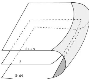
Theǫ-thickeningofSis the tubular neighborhoodTSǫofS:

TSǫ = {q ∈R3: |q−p|≤ǫ, p∈S}

Forǫsmall,Sǫ =∂TSǫis the envelope of the family of spheres of radiusǫand center ranging on S; it is aC1compact boundaryless surface oriented towards the exterior ofSǫ.

This surface is smooth on the complement of the curveBǫ,±which is the inverse image ofB

by the tubular projection π: ˆSǫ → ˆS. In factBǫ,± is the common border of the two connected

smooth surfaces with boundarySǫ,± = S±ǫN (with a connected component for each sign) and

half of the tube centered alongBand radiusǫ, defined parametrically by

Tǫ =B+ǫcosθ N+ǫsinθ N ∧T , 0≤θ ≤π.

See Figure 1 for an illustration of the surfaceSǫ.

Fig. 1 – Thickening of the surfaceS.

Theδ−smoothing ofSǫ is an embedding ofSǫintoR3whose image is a smooth surfaceSǫ,δ which coincides with the identity outside aδ−tubular neighborhood ofBǫ,±.

This surfaceSǫ,δis (not uniquely) defined by averaging the functions

Pǫ =(x−πSˆ(x))

2_−ǫ2_{, forx on b◦π} ˆ S≥0,

and

pǫ=(x−πB(x))2−ǫ2, forx on b◦πSˆ ≤0,

More precisely, take

Pǫ,δ =hδ,ǫPǫ+(1−hδ,ǫ)pǫ

and Sǫ,δ = Pǫ,δ−1(0) where h is a smooth decreasing function in the interval [0, δ] such that

h(n)_(0)=h(n)_{(δ)=0 for alln∈N,h(t )=1 fort ≤0 andh(t )=0 fort ≥δ.}

The principal configuration of the surface Sǫ outside Bǫ,± is known. On one portion it is

provided by that of theTube (Gutierrez and Sotomayor 1991); on the other, i.e. onS−ǫNand S+ǫN, it is obtained from that ofS by translation alongǫNand−ǫN. Notice that sinceSǫ is oriented by its outward normal, the minimal and maximal principal foliation are exchanged in the transition fromS−ǫNtoS+ǫN. For the sake of completeness, the principal configurations on theTubeand translated surfacesS±ǫN are reviewed and established in Section 2.

In this paper it will be proved that, with specific restrictions on the type of transition function

h (see section 3), from points ofC_S of quadratic tangencies of principal lines with_B, bifurcate

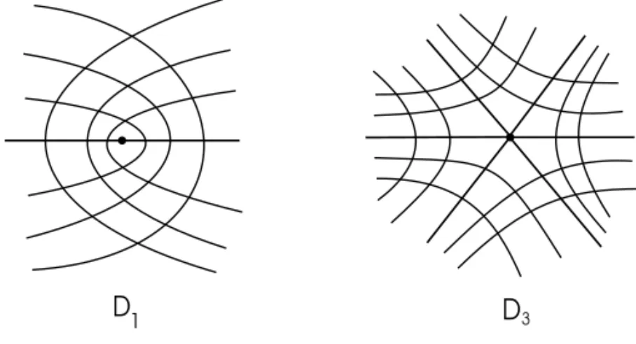
only Darbouxian umbilic points of typesD1andD3onSǫ,δ, forǫandδsmall. See (Gutierrez and Sotomayor 1982, 1991) and Section 4 for the basic properties of Darbouxian Umbilics.

The main result is the following.

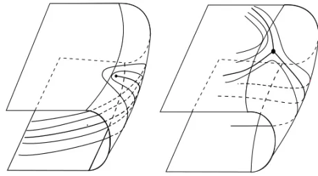
Theorem1. Consider a pointp0ofCSsuch that the minimal (or maximal) principal foliation has quadratic contact (internal or external cases) with the boundary at this point. Then, for appropriate transition functionh, there exists a regular curve of umbilics, tangent toN (p0)and intersecting transversally the surface Sǫ,δ at a point pǫ, for ǫ > 0 (or ǫ < 0) and δ small. This point is a

Darbouxian umbilic point for the surfaceSǫ,δ and it is of typeD1(external tangency case) orD3 (internal tangency case). See Figure 2.

Fig. 2 – Minimal principal foliation ofSǫ,δ: external and internal tangency.

This result expresses the bifurcation phenomenon of transition of tangencies into umbilics on principal configurations, under thickening and smoothing. For smallǫ andδ, tangencies are

transferred into umbilics, from∂StoSǫ,δ.

principal configurations. In the forthcoming paper (Garcia and Sotomayor 2001), is pursued the study of the transition fromP_(S,B)into periodic principal lines on_Sǫ,δ.

From the geometric point of view this work represents a contribution to the analysis of the smooth transition between the two possible principal configurations (one for each orientation) on surfaces with boundary, when passing from one orientation to the other. It is also related to the study of the transition on the phase portrait of a discontinuous differential equation (that of the maximal and minimal curvature lines, one on each side of the surface with boundary), when crossing a line of discontinuity (represented here by the boundary curveB). See the paper by (Sotomayor and Teixeira 1998) dealing with the regularization, i.e. the smoothing, of general discontinuous differential equations.

The fact that the differential equations of principal lines have a geometric realization, one on each side of the surface that carries them, makes it natural to express geometrically the smooth transition between them by means of the surface obtained with the operations of thickening and smoothing defined here.

2 PRINCIPAL CONFIGURATION OF Sǫ

This section provides a self sufficient presentation of the elementary properties of principal con-figurations on surfaces obtained through the thickening procedure from one with boundary.

Let(S,B)be a given surface with boundary, positively oriented by the normal unitary fieldN,

as above. Consider the family of parallel surfacesSǫgiven bySǫ:S+ǫN.

Near a connected component of the borderBwe consider a tube of radiusǫwith center ranging

alongS, as in Figure 1. This procedure defines a boundaryless surfaceSǫ of class onlyC1.

Proposition1. Letc: [0, l] →R3_{be a regular arclength parametrization of a connected} com-ponent ofB, such that{T , N ∧T , N}is a positive frame ofR3_{. Then the expression}

α(u, v)=c(u)+v(N ∧T )(u)+ ₁

2k

⊥

n(u)v

2_+o(v2_{)N (u), −δ < v < δ (1)}

wherek_n⊥is the normal curvature ofSin the direction ofN∧T, defines a localC∞chart on the surfaceSˆ defined in a small tubular neighborhood ofc.

Proof. The map α(u, v, w) = c(u)+v(N ∧T )(u)+wN (u)is a local diffeomorphism in a

neighborhood of the u axis. For each u, the curve v → v(N ∧ T )(u)+w(u, v)N (u) is the

intersection of the surfaceS with the plane spanned by{(N∧T )(u), N (u)}. Using Hadamard’s

lemma it follows that

w(u, v)= ₁

2k

⊥

n(u)v

2_+v2_{A(u, v)N (u)}

whereA(u,0)=0 andk⊥_n is the (plane) curvature of the curve in the plane spanned by{N∧T , N},

Remark1. A similar chart has proved to be useful in (Gutierrez and Sotomayor 1982), for the

study of periodic principal lines, and in (Garcia and Sotomayor 1997), for the analysis of asymptotic lines near parabolic curves.

According to (Spivak 1980), the Darboux frame{T , N∧T , N}alongBsatisfies the following system of differential equations:

T′ = kgN ∧T +knN

(N∧T )′ = −kgT +τgN

N′ = −knT −τg(N ∧T )

(2)

whereknis thenormal curvature,kgis thegeodesic curvatureandτgis thegeodesic torsionof the boundary curveB.

Proposition2. Consider a surfaceSand a connected component of the boundaryBparametrized

byc. Then the principal lines ofSare transversal tocat a pointc(u0)if and only ifτg(u0)=0. Assuming that(k_n⊥−kn)(u0)=(k2−k1)(u0) >0, a minimal principal curvature line has quadratic

contact withcat a pointc(u0)if and only ifτg(u0)=0andτg′(u0)=0.

The contact is internal (respectively external) ifτ_g′(u0) >0(respectivelyτg′(u0) <0).

Proof. Using the parametrization defined by equation 1 and the Darboux frame given by equation

2, it follows that:

E(u,0) = 1, F (u,0)=0, G(u,0)=1

e(u,0) = kn(u), f (u,0)=τg(u), g(u,0)=kn⊥(u)

Therefore the tangent vectorT (u)is a principal direction if and only ifτg(u)=0. From the differential equation of curvature lines

(F g−Gf )dv2+(Eg−Ge)dudv+(Ef −F e)du2=0,

see (Gutierrez and Sotomayor 1991) and (Spivak 1980), it follows that near a point of tangency the minimal principal curvature lines are the solutions of the following differential equation:

u′ = −(k⊥_n −kn)(u0)+ · · ·

v′ = τ_g′(u0)(u−u0)+ · · ·

Therefore,v(u)= −1 2τ

′

g(0)(kn⊥−kn)−1(0)(u−u0)2+ · · ·.

Remark 2. For the maximal principal lines the contact is internal (respectively external) if

(k⊥_n −kn)τg′(u0) <0 ( respectively(k⊥n −kn)τg′(u0) >0).

Proposition3. Consider a surfaceSparametrized near a connected component of the boundary

byαas in equation (1). LetSǫ,+be the parallel surface defined by

Then the principal configurations ofSandSǫ,+are the same, i.e., by a parallel displacement the principal curvature lines, the umbilic points and the tangencies are preserved.

Proof. Direct calculation in any chart(u, v)shows that the coefficients of the first and second

fundamental forms ofSandSǫ,+are expressed as follows:

Eǫ = (1−ǫK)E+(ǫ2H−2ǫ)e

Fǫ = (1−ǫK)F +(ǫ2H−2ǫ)f

Gǫ = (1−ǫK)G+(ǫ2H−2ǫ)g

eǫ = (1−ǫH)e+ǫKE

fǫ = (1−ǫH)f +ǫKF

gǫ = (1−ǫH)g+ǫKG

HereKandHare respectively the Gaussian and Mean Curvature of the surface_S. Therefore,

Fǫgǫ−Gǫfǫ = (1+ǫ2K−ǫH)(F g−Gf )

Eǫgǫ−Gǫeǫ = (1+ǫ2K−ǫH)(Eg−Ge)

Eǫfǫ−Fǫeǫ = (1+ǫ2K−ǫH)(Ef −F e)

Therefore, differential equations of the principal curvature lines ofSandSǫ,+are the same.

This ends the proof.

Remark3. As above, analogous identification of principal configurations, but taking into account

the exchange of maximal into minimal and vise-versa, holds for the surfaceSand that defined by negative translation: αǫ=α−ǫN.This is due to the orientation convention assumed.

Proposition4. Letc: [0, l] →R3_{be a parametrization by arclengthuof a connected component} ofBsuch that{T , N ∧T , N}is a positive basis ofR3_{. Then the expression below}

β(u, θ )=c(u)+ǫcosθ N (u)+ǫsinθ (N∧T )(u) (4)

is a regular parametrization of the tubeTǫof radiusǫcentered at the curvec.

The differential equation of the principal curvature lines is given by

du(dθ −τg(u)du)=0.

At the points whereτg(u0)= 0andτg′(u0) =0the contact between the maximal principal lines

and the curves defined byθ =0andθ =πis of quadratic type.

Proof. The tube centered atcand of constant radiusǫis clearly a regular surface forǫ >0 small.

Using the Darboux frame given by equation (2) and the parametrization (4), it follows that

βu = (1−ǫkncosθ −ǫsinθ )T −ǫτgcosθ N ∧T −ǫτgsinθ N

βθ = −ǫsinθ N+ǫcosθ N∧T

So the coefficients of the first fundamental form are given by:

E = (1−ǫkncosθ−ǫsinθ )2+(ǫτg)2

F = −ǫ2τg

G = ǫ2

As the tube is the envelope of an one parameter family of spheres of radiusǫcentered alongc

the circles parametrized byu=ct eare the minimal principal lines, see (Gutierrez and Sotomayor

1991) and (Spivak 1980). Here the positive orientation of the tube is defined by the exterior normal, having the circlesu=ct eprincipal curvaturek1= −1_ǫ. Therefore, the orthogonal family of curves, the other family of principal lines, is defined by the integral curves of the vector field

X=G_∂u∂ −F_∂θ∂ or equivalently by the differential equation dθ_du = −F

G =τg(u). A solution of the equation above has the following Taylor expansion

θ (u)=θ0+1 2τ

′

g(u0)(u−u0)2+ · · ·.

This ends the proof.

Proposition 5. Consider the boundaryless surface Sǫ obtained from a surfaceSby a parallel

displacement of distanceǫ in both normal directions, glued to each other by the half tubesTǫ of

radiusǫ >0centered along the boundaryBofS. Then for smallǫ, the surfaceSǫ =Sǫ,+∪Tǫ∪Sǫ,− is smooth outside the curvesB±ǫN and regular of classC1along these curves.

The principal foliations lines ofSǫare as follows:

1. The minimal principal lines ofSǫ, away from tangencies, are the minimal principal lines of Sǫ,+, together with the minimal principal lines of the tubesTǫ(semi circles) and the minimal

principal lines of the surfaceSǫ,−. These last mentioned curves are the parallel translation of

the maximal principal ones ofS.

2. The maximal principal lines of Sǫ, away from tangencies, are the maximal principal lines

of Sǫ,+, together with the maximal principal lines of the tubes Tǫ (curves defined by the

differential equationdθ −τgdu = 0) and the maximal principal lines of the surface Sǫ,−. These last mentioned curves are the parallel translation of the minimal principal ones ofS. See Figure 3.

Proof. In this situation the tubeTǫ is glued toSǫ,+ atθ =0 and toSǫ,−atθ = π. The tube is

oriented positively with normal exterior andSǫ,−has orientation opposite ofSǫ,+. The minimal

(respectively maximal) principal lines ofSǫ,−are obtained by parallel displacement of the maximal

(respectively minimal) principal lines ofSǫ,+.

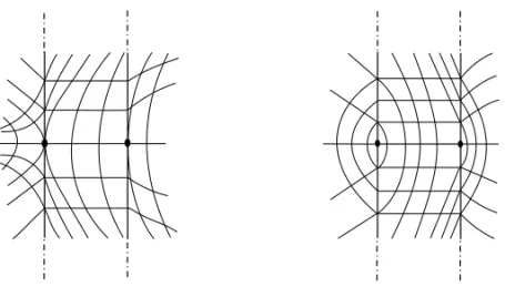
Fig. 3 – Piecewise Smooth Principal configuration ofSǫ: internal and external tangency.

(resp. maximal) tangencies with Bǫ when ǫ > 0 (resp. when ǫ < 0). The piecewise smooth leaves are defined by continuation of the principal lines on the tube and parallel surfaces, crossing throughSǫ,±. In this context the external,E, and internal,I, minimal tangencies give rise to local

configurations topologically equivalent to those aroundD1andD3umbilics.

Recall that the main result of this paper establishes that by a suitable smoothing the piecewise smooth principal configuration is deformed into a smooth one for which curves of ‘‘new’’ umbilics appear along arcs which are tangent toEandI. Furthermore, the umbilics are Darbouxian of types D1andD3, respectively. See Figures 2 and 3 for an illustration of the principal configuration in Sǫ,δandSǫ.

3 SMOOTHING OF SǫIN A LOCAL CHART

In this section will be studied the principal configurations of the smoothing of the surfaceSǫ by the operation ofδ−smoothing. To this end consider an appropriate local chart(u, v).

Proposition6. Letc: [0, l] →R3_{be a parametrization by arclengthuof a connected component} ofBǫsuch that{T , N∧T , N}is a positive frame ofR3. Then the expression

β(u, v)=c(u)+v(N ∧T )(u)+−ǫ+ǫ2−v2

N (u) (5)

defines a regular parametrization of the tubeTǫ of radiusǫcentered at the curvec−ǫN.

Proof. Direct by the parametrization of the circle in the plane{N∧T , N}.

Proposition7. Consider the surfaceSǫwith boundaryBǫ. Then the surfaceSǫhas the following

parametrization

βǫ(u, v) = c(u)+v(N ∧T )(u)+R(u, v, ǫ)N (u), 0< v < δ,

αǫ(u, v) = c(u)+v(N ∧T )(u)+S(u, v, ǫ)N (u), −δ < v≤0,

where,

R(u, v, ǫ) = −ǫ+ǫ2−v2, 0< v < δ

S(u, v, ǫ) =k_n⊥v 2

2 +a(u, ǫ)

v3

6 + · · ·, −δ < v≤0.

Herek⊥_n =k_n⊥(u, ǫ)is the normal curvature ofBǫ=B+ǫN anduis the arc length ofc.

Proof. Similar to that of proposition 1.

Remark4. The principal curvatures ofSandSǫ are related by:

k2(ǫ)= k2

1+ǫk2, k1(ǫ)

= k1 1+ǫk1

The extensions ofβǫandαǫ, given by equation 6, in a neighborhood ofc, i.e., for −δ < v < δ, it will be supposed in the following.

Lethbe a smooth function defined inRsatisfying the properties,_h|−∞,0) =1, h|δ,∞) = 0 andhdecreasing in the interval[0, δ].

An example of suchhis given by the following.

Let

ψ (v)=  



0, for v≤0

e−av, for 0< v≤δ

Definehby,

h(v)= ψ (δ−v)

ψ (v)+ψ (δ−v) (7)

Also consider the function

H (v)= −1+h+2vhv+ 1 2v

2_h

vv= −

(1−h)v 2

2

vv

that will appear in the proof of Theorem 1. See section 4 and equation 13.

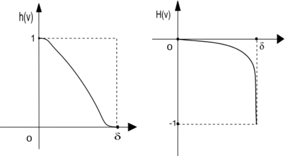
Proposition8. Consider the functionH (v)= −1+h+2vhv+₂1v2hvvdefined in the interval [0, δ]. Then for an appropriate transition functionhit follows thatH (v) <0for allv∈(0, δ].

Proof. Let

ψ (v)=  



0, for v ≤0

e−av, for 0< v ≤δ

Define

h(v)= ψ (δ−v)

ψ (v)+ψ (δ−v)

Plotting the graphs ofh andH it follows that fora > 0 small enoughhhas the properties

mentioned above andH|(0,δ)is negative. See Figure 4. This numerical assertion can be corroborated by an asymptotic analysis ina >0.

In fact, ashis strictly decreasing in the interval[0, δ]and is concave near 0, i.e.,hvv(v) <0, it follows thatH is strictly decreasing in an interval [0, ρ(a, δ)] withH (0) = 0 and having all derivatives equal to zero atv=0.

The functionH has the following asymptotic expansion ina.

H (v, a, δ)= −1

2 +

1 4

δ3−4vδ2+4v2δ−2v3

v(δ−v)3 a+o(a 2_).

In a compact interval[ρ(a, δ), δ]the function

Ha(v)= 1 4

δ3−4vδ2+4v2δ−2v3 v(δ−v)3 =

1 4

1

v +

vδ−v2−δ2 (δ−v)3

is negative ifδis small.

Therefore, it follows that fora >0 andδ > 0, both small, the functionH is negative in the

interval[0, δ], as asserted.

Fig. 4 – Transition functionhand functionH.

Remark5. The functionH (v)= − (1−h(v))v₂2

vvis proportional to the curvature of the plane curve C(v) = v, (1−h(v))v₂2. For an appropriated h as considered aboveH is negative if a >0 is sufficiently small.

Consider the parametrization of the surface Sǫ given by equation 6 and consider the

δ−smoothing

γ (u, v, ǫ)=αǫ(u, v)h v

ǫ2

+1−h v

ǫ2

Direct calculation shows that

γ (u, v, ǫ) =c(u)+v(N∧T )(u)

+

h(v ǫ2)

k_n⊥v

2

2 +a(u, ǫ)

v3

6 + · · ·

+ 1−h v

ǫ2

−ǫ+ǫ2−v2

N (u)

(9)

Now consider the rescalingv=ǫ2v¯ in the expression above and rewriting back(v= ¯v), it is

obtained that

γ (u, v, ǫ) =c(u)+ǫ2v(N ∧T )(u)+A(u, v, ǫ)N (u)

=c(u)+ǫ2v(N ∧T )(u)

+

ǫ4h(v)

k⊥_n v 2

2 +ǫa(u, ǫ)

v3

6 + · · ·

+ǫ[1−h(v)] −1+1−ǫ2v2

N (u).

(10)

The non unitary normal vector toSǫ is given by

¯

N =(N1, N2, N3)=N1T (u)+N2(N ∧T )(u)+N3N (u)

where,N1=(a2b3−a3b2)/ǫ2, N2=(a3b1−a1b3)/ǫ2,N3=(a1b2−a2b1)/ǫ2and

a1 = 1−ǫ2kgv−knA b1 = 0,

a2 = −τgA, b2 = ǫ2,

a3 = Au+ǫ2τgv, b3 = Av.

Let

a11 = ∂a1

∂u −kga2−kna3, a21 = −ǫ 2_k

g−knAv, a31 = 0,

a12 = ∂a2

∂u +kga1−τga3, a22 = −τgAv, a32 = 0,

a13 = ∂a3

∂u +kna1+τga2, a23 = ǫ 2_τ

g+Auv, a33 = Avv.

Therefore,

γuu = a11T +a12N∧T +a13N

γuv = a21T +a22N∧T +a23N

γvv = a31T +a32N∧T +a33N

The coefficients of the first fundamental form ofγ are given by:

E = γu, γu = a₁2+a₂2+a₃2

F = γu, γv = a1b1+a2b2+a3b3

The coefficients of the second fundamental form ofγ are proportional to the following

func-tions:

e = γuu, γu∧γv = a11N1+a12N2+a13N3

f = γuv, γu∧γv = a21N1+a22N2+a23N3

g = γvv, γu∧γv = a31N1+a32N2+a33N3

Direct calculation shows that:

E(u, v, ǫ) = 1−2ǫ2kgv+ǫ3kn(1−h)+ǫ4v2(τg2+k2g−knkn⊥h)+ǫ6(· · ·)

F (u, v, ǫ) = 1 12ǫ

5_v21

2τg(−1+h+vhv)+ 1 2ǫτ k

⊥

n(h+vhv)+ǫ2v(· · ·)

G(u, v, ǫ) = ǫ4

1+1 4ǫ

2_v2_(vh

v+2h−2)2+ǫ4v2(· · ·)

(11)

e(u, v, ǫ) =kn+ǫkgv

1−h−1 2vhv

+1 2ǫ

2_v

2τ′−kg(4kn+2kn⊥h+k

⊥

nvhv)

+ǫ3(· · ·)

f (u, v, ǫ) =ǫ2τg+ǫ4v

(k⊥_n)′v 1

2vhv+h

+τgv2(h−1+vhv)2

+ǫ6(· · ·)

g(u, v, ǫ) =ǫ3

−1+h+2vhv+ 1 2v

2_h

vv

+ǫ4kn⊥

h+2vhv+ 1 2v

2_h

vv

+ǫ5v(· · ·)

(12)

Therefore it is obtained:

L(u,0, ǫ) = (F g−Gf )(u,0, ǫ) = −ǫ6τg

M(u,0, ǫ) = (Eg−Ge)(u,0, ǫ) = ǫ4(k_n⊥−kn)

N (u,0, ǫ) = (Ef −F e)(u,0, ǫ) = ǫ2τg

It follows that:

L(u, v, ǫ) =ǫ6−τg+ǫ2v(· · ·)

M(u, v, ǫ) =ǫ3

−1+h+2vhv+ 1 2v

2_h

vv

+ǫ4

k_n⊥−kn+kn⊥

−1+h+2vhv+ 1 2v

2_h

vv

+ǫ5v(· · ·)

N (u, v, ǫ) =ǫ2τg+

ǫ4

4 v

(4h+2vhv)(k⊥n)

′_+τ

g(h2vv

3_−4v2_h

v+4v2hhv

−8vh+4v+4vh2−8kg)

+ǫ5(· · ·)

(13)

4 PROOF OF THE MAIN RESULT

Let 0 be an umbilic point of a C4 immersion α parametrized in a Monge chart (x, y)by α(x, y)=(x, y, h(x, y)), where

h(x, y)= k 2(x

2_+y2₎₊a

6x

3₊b

2xy

2₊ c

6y

3_+O(4)

The differential equation of principal curvature lines is given by:

−[by+P1]dy2+ [(b−a)x+cy+P2]dxdy+ [by+P3]dx2=0

wherePi,i=1,2,3, represent functions of orderO(x2+y2). Let

=P =4b(a−2b)3−c2(a−2b)2

Proposition9 (Gutierrez and Sotomayor 1982, 1991). Under the conditions above suppose that

the transversality conditionT =b(b−a)=0holds and consider the following situations:

D1) =P >0

D2) =P <0and

a b >1

D3) a b <1

Then each principal foliation has in a neighborhood of0, one hyperbolic sector in theD1case, one parabolic and one hyperbolic sector inD2case and three hyperbolic sectors in the caseD3. The umbilics are called Darbouxian of typesD1,D2andD3.

See Fig. 5 for illustrations ofD1andD3. The typeD2does not appear in this work.

Fig. 5 – Darbouxian umbilic pointsD1andD3.

Proof. Solving the equationN (u, v, ǫ)=0 it follows, by Implicit Function Theorem, that there exists a smooth functionu(v, ǫ)such thatN (u(v, ǫ), v, ǫ)=0 and

u(v, ǫ)=ǫ2ξ(v, ǫ), ξ(0)=0.

Therefore the equationM(u, v, ǫ)=0 is such thatM(u(v, ǫ), v, ǫ)=M(v, ǫ)=0. Applying the Implicit Function Theorem to this equation it follows that there exists a smooth function of the formǫ =ϕ(v),where

ϕ(v)= (1−h−2vhv−1/2v

2_h

vv)

(kn−kn⊥)(u0)

[1+ · · · ]

withM(v, ϕ(v))=0, ϕ(0)=0 and is a flat function atv=0. By the properties of the transition functionh, it follows thatϕis decreasing forv >0 small. So it follows thatv=ϕ−1(ǫ).

Returning to the original coordinates(u, v, ǫ), recalling thatv = ǫ2v¯ and sov¯ =ϕ−1(ǫ), it

follows thatv=ǫ2ϕ−1(ǫ). Therefore the curve of umbilic points is given by

U_(ǫ)=(ǫ2_ξ(ǫ2_ϕ−1_{(ǫ), ǫ), ǫ}2_ϕ−1_{(ǫ), ǫ).}

Direct calculation givesU′₍0₎=(0,0,1)=N (c(u0)).

Proposition10. Suppose thatτg(0) = 0,τg′(0) = 0and(kn⊥−kn)(0) >0. Then the curve of

umbilic pointsγ (U_{ǫ)is tangent to the normal vector N (c(u0))and is transversal to the surface} Sǫ,δ in a neighborhood of this point of tangencyc(u0). This intersection point is an umbilic point of typeD1orD3according toτ_g′(0) <0(external tangency) orτ_g′(0) >0(internal tangency). The principal configuration is regular nearc(0)−ǫN.

Proof. The umbilic points of the surfaceγ are given by equation 13,L(u, v, ǫ)=M(u, v, ǫ)=

N (u, v, ǫ)=0.

By Lemma 1, near an umbilic point(0, v1), it follows that

L(u, v, ǫ) = −ǫ6τ_g′(0)u+o(2)

M(u, v, ǫ) = ǫ(k⊥_n −kn)′(0)u+b(ǫ)(v−v1)+o(2), b(0)=b0 <0

N (u, v, ǫ) = τ_g′(0)u+o(2)

whereb0= ∂H

∂v(v1) <0.

The differential equation of curvature lines is given by,

−τ_g′(0)ǫ2u+o(2)dv2+ǫ2ǫk0u+b(ǫ)(v−v1)+o(2)dudv+

τ_g′(0)u+o(2)du2=0

wherek0=(k⊥n −kn)′(0).

By the classification of Darbouxian umbilic points, Proposition 9, it follows that the tangent to the umbilic separatrices are defined byu=λv, where

λτg′(0)λ2+ǫ3k0λ+ǫ2(b−τg′(0)ǫ2)

Therefore the discriminant of the equation above is given by

==ǫ2

−4bτ_g′(0)+4ǫ2(τ_g′(0))2+ǫ4k₀2 .

So, ifτ_g′(0) >0 it follows that= >0 and the umbilic point is of the typeD3.

On the other hand, ifτ_g′(0) <0 it follows that= <0 and the umbilic point is of the typeD1.

Near the pointc(0)−ǫN, since the orientation is exchanged it follows thatkn⊥(0, ǫ)−kn(0, ǫ) <0 and thenM(u, v, ǫ) = 0 in a neighborhood of this point. Therefore the principal foliations are

regular there.

Remark6. The main result of this paper shows that from a quadratic tangency the Darbouxian

umbilic of typeD2does not appear in the process of thickening and smoothing.

5 CONCLUDING REMARKS

A global result, relating quadratic tangencies, Darbouxian umbilic points and the Euler-Poincaré characteristic of the surface is given by the following proposition.

Proposition11. Consider a compact, oriented surfaceSwith regular boundaryBsuch that all

umbilic points of S are Darbouxian and the tangencies, internal and external, of the principal foliationsF_{1S and}F_{2S with the boundary at}C_{Sare quadratic. Then the following expression for} the Euler-Poincaré characteristic forSandSǫ,δ holds:

χ (Sǫ,δ)=2χ (S)=2

#(D1)+#(D2)−#(D3)+ #(E)−#(I ) 2

,

where #(Di), i = 1, 2, 3, is the number of umbilic points of typeDi and #(E), #(I ) are,

respectively, the number of external and internal tangencies of both principal foliations with the boundaryB.

Proof. The proof follows recalling thatχ (Sǫ,δ)=χ (Sǫ)=2χ (S)and thatχ (Sǫ,δ), by Poincaré-Hopf Theorem, is equal to the sum of the indices of the singularities of principal curvature line field

L_1S, see (Spivak 1980) and also (Garcia et al. 2000), and that near a point of quadratic tangency

bifurcate a Darbouxian umbilic point of type D1 or D3, according the tangency is external or

internal.

ACKNOWLEDGMENTS

RESUMO

Neste trabalho são estudadas as linhas de curvaturas principais de uma superfície com bordo e da superfície regular, sem bordo, obtida pelo processo de engrossamento e regularização. É analisada a relação entre as tangências quadráticas das folheações principais com o bordo e os pontos umbílicos Darbouxianos, da superfície sem bordo, que bifurcam dos referidos pontos de tangências.

Palavras-chave: configuração principal, pontos umbílicos, singularidade tangencial.

REFERENCES

Darboux G.1896. Leçons sur la Théorie des Surfaces, vol. IV. Sur la forme des lignes de courbure dans la voisinage d’un ombilic, Note 07, Paris: Gauthier Villars, 420p.

Garcia R and Sotomayor J.1997. Structural stability of parabolic points and periodic asymptotic lines, Matemática Contemporânea, 12: 83–102.

Garcia R and Sotomayor J.2000. Lines of Axial Curvature on Surfaces Immersed inR4, Differential

Geometry and its Applications, 12: 253–269.

Garcia R and Sotomayor J.2001. Periodic behavior of principal curvature lines on surfaces with boundary, in preparation.

Garcia R, Gutierrez Cand Sotomayor J.2000. Lines of Principal Curvature around Umbilics and Whitney Umbrellas, Tohoku Math J, 52: 163–172.

Gutierrez Cand Sotomayor J.1982. Structural Stable Configurations of Lines of Principal Curvature, Asterisque, 98-99: 185–215.

Gutierrez Cand Sotomayor J.1991. Lines of Curvature and Umbilic Points on Surfaces, Brazilian 18th Math. Coll., Rio de Janeiro: IMPA, 112p. Reprinted as Structurally Configurations of Lines of Curvature and Umbilic Points on Surfaces, Lima: Monografias del IMCA.

Gutierrez Cand Sotomayor J.1998. Lines of Curvature, Umbilical Points and Carathéodory Conjecture, Resenhas IME-USP, 3: 291-322.

Melo W and Palis J.1982. Geometric Theory of Dynamical Systems, New York: Springer Verlag, 320p.

Sotomayor J and Teixeira M. 1998. Regularization of Discontinuous Vector Fields, International Con-ference on Differential Equations (Equadiff 95), Word Scientific Publishing Co. p. 207-223.