DOI: http://dx.doi.org/10.1590/2446-4740.02815
*e-mail: [email protected]
Received: 21 September 2015 / Accepted: 10 February 2016
On the geometric modulation of skin lesion growth: a mathematical
model for melanoma
Ana Isabel Mendes*, Conceição Nogueira, Jorge Pereira, Rui Fonseca-Pinto
Abstract Introduction: Early detection of suspicious skin lesions is critical to prevent skin malignancies, particularly the melanoma, which is the most dangerous form of human skin cancer. In the last decade, image processing techniques have been an increasingly important tool for early detection and mathematical models play a relevant role in mapping the progression of lesions. Methods: This work presents an algorithm to describe the evolution of the border of the skin lesion based on two main measurable markers: the symmetry and the geometric growth path of the lesion. The proposed methodology involves two dermoscopic images of the same melanocytic lesion obtained at different moments in time. By applying a mathematical model based on planar linear transformations, measurable parameters related to symmetry and growth are extracted. Results: With this information one may compare the actual evolution in the lesion with the outcomes from the geometric model. First, this method was tested on predeined images whose growth was controlled and the symmetry known which were used for validation. Then the methodology was tested in real dermoscopic melanoma images in which the parameters of the mathematical model revealed symmetry and growth rates consistent with a typical melanoma behavior. Conclusions: The method developed proved to show very accurate information about the target growth markers (variation on the growth along the border, the deformation and the symmetry of the lesion trough the time). All the results, validated by the expected phantom outputs, were similar to the ones on the real images.
Keywords: Digital image skin processing, Melanoma, Segmentation, Dermoscopy, Linear transformations.
Introduction
Cancer and related diseases remain a major issue to the scientiic community. Due to the nature of the underlying process of carcinogenesis, several multicenter teams have been making efforts to further understand the process (at the molecular, cellular and tissue levels). The research in cancer provides evidence that an interdisciplinary approach brings empowerment to research, and this is an important contribution to what we know today about cancer and carcinogenesis.
Despite being the rarest among all skin cancers, the melanoma is one of the most deadly forms of the disease (Longo et al., 2012). Melanoma is a skin cancer derived from the melanocytes, cells that produce melanin, the skin coloration pigment.
The United States epidemiology of cancer laid skin cancer as the most common form of malignancy over the past three decades (Rogers et al., 2010; Stern, 2010). In particular the melanoma is also the most common form of cancer for young adults (25-29 years old) and the second most common form of cancer for young people (15-29 years old) (Bleyer et al., 2006).
European studies have documented an increase of melanoma incidence in the last few decades (Baumert et al., 2009; Downing et al., 2006; Holterhues et al., 2010; Sant et al., 2009; Tryggvadóttir et al., 2010). In the case of Portugal, the estimated incidence for 2012 was 7.5 per 100 000, mortality 1.6 per 100 000 and prevalence at one, three and ive years at 12.08%, 33.99% and 53.93% respectively (Ferlay et al., 2013).
Due to the high malignancy potential of melanoma, early detection of suspicious skin lesions is critical to prevent malignancy and to increase the treatment eficacy (Whiteman et al., 2011).
Dermoscopy is a non-invasive imaging technique used to obtain digital images on the skin surface by using a device known as dermoscope. It comprises a magnifying lens and a light source attached to a digital camera. This device allows the visualization of pigmented structures or vessels in the epidermis and supericial dermis (Zalaudek et al., 2010). Most dermoscopic structures are correlated with speciic histopathological markers, therefore dermoscopy can be regarded as a link between clinical (macroscopic) and histopathological (microscopic) morphology (Zalaudek et al., 2006b).
Dermoscopy has been successfully applied since the early 1990’s. Some examples of the irst works can be found in (Benelli et al., 1999; Dal Pozzo et al., 1999; Menzies et al., 1996; Skender-Kalnenas et al., 1995; Soyer and Kerl, 1993; Soyer et al., 1995). Digital image processing applied to dermoscopic images is an important tool to improve naked eye evaluation, increasing sensibility and speciicity to diagnose (Andreassi et al., 1999; Menzies et al., 1996; Piccolo et al., 2002). The use of image processing techniques enabled quantiication, pre-processing (enhancing contrast, alignment, among others), eliminate common artifacts (Abbas et al., 2011; 2013; Afonso and Silveira, 2012; Fonseca-Pinto et al., 2010) and extract quantitative features to classify structures (Andreassi et al., 1999; Soyer et al., 1995) to establish a measure of malignancy associated to the lesion, as proposed in (Abbas et al., 2013; Argenziano et al., 2011; Blum et al., 2003; Piccolo et al., 2014; Şavk et al., 2004; Zalaudek et al., 2006a). These techniques also allow the use of automated classiication of skin lesion, which is a valuable help to clinical practice (Cheng et al., 2013; Liu et al., 2012).
Among all features that we can extract from images, as a consequence of the carcinogenesis evolution, the lesion growth is of particular relevance. Although this is not the only symptomatic feature, the growth and growth rate pattern of the lesion is one of the most valuable signs of malignancy, and can be studied using mathematical models that quantify and classiies the growth pattern. The combination of image processing techniques with mathematical models is a strategy with an important role to map the progression of lesions.
This work presents an algorithm based on linear transforms that evaluates the evolution of the border of the skin lesions based on two main measurable markers: the symmetry and the geometric growth path of the lesion. These markers are obtained through the relation between two segmented dermoscopic images of the same melanocytic lesion, obtained at different moments in time.
After this introduction of the problem, the remaining sections of this article are organised as follows: In the methodology and image setting section, methodological questions related to the image pre-processing are presented and the steps of the mathematical model are described. Then, in the section of results, the model is applied to a set of images (phantoms and real images). The work ends with the discussion and conclusions section, presenting the analysis of the results and concluding with the future perspectives in the context of the mathematical modelling of growth lesions in skin cancer, suggesting in perspective an
individual signature model, in which growth and symmetry plays a pivotal role.
Methods
Dermoscopic images are obtained in the context of a clinical examination, and can be affected by some lack of time imposed by economic and human constrains. These and other aspects can affect the quality of the acquired image. Also the presence of hairs and air bubbles (when a luid is applied in the interface between the dermoscope and the skin) requires a pre-processing step to assemble the image to the segmentation. The segmentation, being the irst step in the image analysis, requires a robust methodology, since the remaining process depends on its accurate output.
A wide range of algorithms has been used for image segmentation, broadly categorized as pixel-based segmentation, region-based segmentation and edge detection (Joel et al., 2002; Mendonca et al., 2007; Sadri et al., 2013; Toossi et al., 2013; Wang et al., 2010).
The method used to segment images in this work was irstly proposed for dermoscopy in (Pereira et al., 2015), and uses the Multiscale Local Normalization (MLN) methodology. The use of a Gaussian kernel to the image in MNL overcomes the image perception dependence on the surroundings.
Matlab® software was used to implement the model presented in this work. It was used also in the construction of a set of binary images.
Real dermoscopic images used to test the methodology were obtained in the context of clinical practice by a dermatologist in a public hospital, with a previous informed consent to use these images for research purposes.
Image dataset
Image registration
According to what has been stated above, two images of the same lesion, obtained in two separate moments, were used to establish a marker of growth. It cannot be guaranteed that both images are captured exactly in the same conditions, i.e., the angle of incidence, light scattering and skin properties, among others. These different conditions may induce errors in the quantiication of growth, caused by non-aligned pairs of images. In order to minimize these errors, a process of image registration was performed.
In this step the goal is to obtain the best alignment between both images. Hence, both images are aligned by their centroids. Among all possible senses for best
alignment (mathematical, morphological, biological), taking into account the kind of images and the context of its acquisition, the global shape marker is used to achieve this matching, as described in the following.
The adjustment is performed by rotating the image taken in time one, It
1, over the image taken in time zero, It
0, and simultaneously calculating the standard deviation between them, deined by
( ) (2 )2 0
n
i i i i
i
x x y y
=
s = ∑ − ′ + − ′ (1)
where (x yi, i) and
( )
', ' i ix y are respectively the points of the border of It
0 and It1 obtained by the segmentation process.
The best adjustment is obtained by minimizing the standard deviation. In Figure 2 it is possible to observe an example of this adjustment in which (Equation 1) is minimized.
Border points
In order to optimize the process, an equally-spaced undersampling approach is performed on the border of the lesion It
0. This allows reducing the amount of data that the algorithm works, while preserving all the essential information, which basically is the lesion shape. For each of the selected points in It0, there must be a correspondent one in I
t1. Those matching points are selected to be the nearest points to the respective one in the border of I
t0 (see Figures 3a and b). In some cases, where the distance between border I
t1 candidates is abnormal (see Figure 3c), another approach is required. Normal/abnormal distances were classiied according to previous simulation studies in other melanocytic images (Ferlay et al., 2013) from different image databases. In abnormal distances cases, the points will be selected as the intersection between the I
t0 border and a line that passes through the centroid (x y0, 0)and the point ( )x y, in It
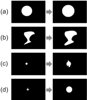
0. Figure 1. Phantom examples for growth simulation (a) preserving the
shape; (b) maintaining shape but not proportional in every direction; (c) and (d) changing shape.
Figure 2. Example of image registration. Left: Images It
Global growth rate
The Global Growth Rate (GGR) deined in (2) reports information about the overall lesion growth behavior computing relative measures between the undersampled points. This rate is deined by
( ) ( )
0
2 2
i i i i
x' x y' y
i
i
d
GGR
max
− + −
= (2)
where di0= (xi−x0) (2+ yi−y0)2 and 1,i= …,M for a sampling with M points where the points (x yi, i),
( )
' ',
i i
x y and (x y0, 0)are respectively points in the border of It
0, the corresponding points in the border of It1 and the centroid.
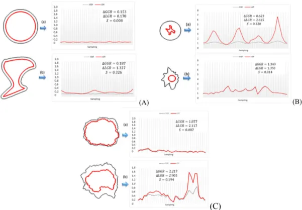
The different behavior of GGR is presented on Table 1A, where, T1 = 0 in lesions with absence of growth, for all i = 1,…,M, is obtained directly from the GGRi expression, because if there is no growth then the numerator in (Equation 2) is zero for every i. To detect growth, the values of GGRi, i = 1,…,M, must be different than zero for one sample of these values. The deviation of GGR={GGR :i i= …1 , , M}, denoted by ∆GGR, was also computed in order to verify if the lesion grows globally the same distance along each point on the border, and is given by (Equation 3).
( ) ( )
max GGR min GGR
GGR
GGR −
∆ = (3)
where GGR denotes the average of GGR.
In Table 1B, T2 = 0.2 is obtained by experimental results between predicted and labeled phantom behavior. For every ∆GGR below this number is assumed to represent a lesion with a non-signiicant variation of the GGR values, therefore being labeled as having
the same growth along the border. Otherwise, they are labeled as lesions with variation on the growth along a sample of points of the border.
Local growth rate
The Local Growth Rate (LGR) presented in (Equation 4) gives information on how the lesion grows locally and is given by
( ) (2 )2 0
'i i 'i i
i
i
x x y y
LGR
d
− + −
= (4)
If the lesion has a regular local growth behavior then it indicates absence of shape alterations. In other words, growth has been also proportional through time in every direction in relation to local dimensions. Otherwise, on the presence of irregular local growth, the lesion suffered deformation. If the deformation is small, it is not possible to detect alterations with naked eye, as presented in the example of Figures 5A and B.
This deformation is quantiied by the deviation of LGR={LGR ii : 1= … , , M}, denoted by ∆LGR, which is deined in (Equation 5).
( ) ( )
max LGR min LGR
LGR
LGR −
∆ = (5)
where LGR denotes the average of LGR.
In Table 1C, T3 = 0.2 is obtained by experimental results between predicted and labeled phantom behavior. For every ∆LGR bellow this number is assumed to have a non-signiicant variation of the LGR values, therefore being labeled as a lesion with maintained proportion. Otherwise, they are labeled as lesions with deformation.
Figure 3. Point detection approach in the border of image It
1. (a) and (b) by selecting the nearest points of It0, and (c) using radial lines as
reference. Those matching points are selected to be see Figure 3a and b. In some cases, where the distance between border I
t1 candidates is
Circularity
Circularity values deined in (Equation 6) inform about the circular type of the lesion in time zero, It
0 and it is denoted by S and deined by the statistical coeficient of variation (CV) of elements in the set of coeficients between local and global growth, CLG.
( ) CLG
S CV CLG
CLG s
= = (6)
where CLG denotes the average of elements of CLG,
s
CLG denotes the standard deviation of the elementsCLG, with CLG deined by CLG={CLGi :i= …1, ,M}, for
i i
i
LGR CLG
GGR
= .
As mention, circularity data informs about the circular type of the shape of the lesion in It
0 and cannot have negative values. If GGR and LGR curves results have similar behavior then the lesion in It
0 must have a circular type shape as both local and global distances produce the same results. In fact, the elements in the set CLG will mostly be 1. Therefore the value of S is closer to 0, which means there is no variability in the data in CLG. It is also possible to check information about the regularity of the shape of the lesion It
1, if in expressions (Equation 2) and (Equation 4) we
replace di0 by
(
') (
2 ')
21 0 0
i i i
d = x −x + y −y . In this case,
we analyze the circularity shape of the lesion It
Every lesion with circularity below this number is assumed to have a signiicant relation between LGR
and GGR, therefore it is labeled as a circular type shape lesion. Otherwise, it is labeled as a non-circular shape lesion.
Symmetry coeficients
Symmetry is widely used to access the potential evolution from naevus to melanoma in dermoscopy skin evaluations. In order to access the lesion symmetry as an overall marker, the Angular Coeficient of Symmetry (ACS) is computed for each pair of images (It
0 and It1). To calculate this coeficient an orthonormal reference system is considered whose origin coincides with the centroid of the image. Next it is obtained a symmetry linear transformation over the y-axis, as deined in (Equation 7).
' 1 0
' 0 1
x x
y y
−
=
(7)
where (x, y) are lesion points in the 1st and 4th quadrants. Next an overlapping between (x y′, ') and the lesion points on the 2nd and 3rd quadrants is obtained. Since the image is binary, after these overlapping, the inal result will display 0, 1 or 2 for pixel values. Pixels with 0 indicate non-lesion with non-lesion overlapping, pixels with 1 indicates lesion with non-lesion overlapping and for those pixels with value 2, this indicates lesion with lesion overlapping. The relevant information is given by the relation between the frequencies of the pixel value 2 over 1. The higher the relative presence of 2, the higher the symmetry response, which is deined in (Equation 8).
2 1 2 y z SC z z =
+ (8)
where zj = total number of values j in the 2nd and 3rd quadrants, j∈ 1, 2{ }.
The symmetry over the x-axis is obtained using a linear transformation deined in (Equation 9) by
' 1 0
' 0 1
x x
y y
=
−
(9)
where (x, y) are lesion points in the 1st and 2nd quadrants. In the following an overlapping between (x y′, ') and the lesion points on the 3rd and 4th quadrants is obtained. As in the former case a coeficient of symmetry SCx
is computed and deined in (Equation 10).
2 1 2 x z SC z z =
+ (10)
where zj = total number of values j in the 3rd and 4th quadrants, j∈ 1, 2{ }.
The symmetry coeficients were obtained through decile rotations of the image to complete 360 degrees. In each iteration of the process results for angles
10 , 20 , , 360
θ = ° ° … ° we calculate two values SCxθand .
y
SCθ Next, using the previous values at distinct angles, the ACSθi is given in (Equation 11) by
{
}
– , 10 , 20 , 30 , , 360 2
i i i i
i
x y x y
i
SC SC SC SC
ACSθ θ θ θ θ ° ° ° °
+ −
= θ ∈ … (11)
Finally, taking ACS
{
ASCi : i 1 0 , 20 , 30 , , 360}
° ° ° °
θ
= θ = … ,
a single value for Angular Coeficient of Symmetry is obtained by the average of the previous angular coeficients of symmetry, denoted by ACS.
ACS can be used for quantitative and qualitative proposes, depending on the goal. For a qualitative usage, a threshold value is set in order to deine the lesion as either symmetric or asymmetric, using the decision Table 1E. Otherwise, if the intent is to obtain a more discriminant measure, the value of ACS for each lesion may be used.
In Table 1E, T5 = 0.8 is obtained from experimental results between predicted and labeled phantom behavior. Every lesion with ACS above this number is assumed to have a signiicant symmetry along their rotation, therefore it is labeled as a symmetric lesion. Otherwise, it is labeled an asymmetric lesion.
The deviation of ACS, denoted by ∆ACS, and given by (Equation 12) was also computed in order to correlate this results with the ones obtained for the regularity of the shape in circularity. If the deviation of ACS is small, that means that the ACS along the lesion is fairly constant, therefore the lesion must have circular shape with possible small variations along the border. Otherwise, it means the lesion has a non-circular shape. So when facing lesions with these characteristics, the decision should match the obtained previously on the circularity.
( ) ( )
max ACS min ACS
ACS
ACS −
∆ = (12)
In Table 1F, T6 = 0.2 is obtained by experimental results between predicted and labeled phantom behavior. Every lesion with ∆ACS below this number is assumed to have a non-signiicant variation of their symmetry; therefore it is labeled as a circular type shape lesion. Otherwise it is labeled as non-circular type shape lesion.
Results
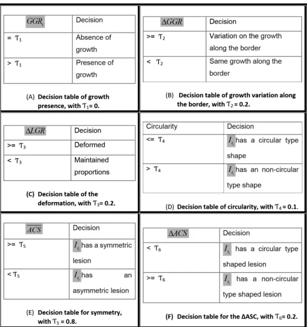
In Figure 4 there are two examples of lesions with absence of growth. There is a circular type shape phantom lesion in Figure 4a and a non-circular type shape phantom lesion in Figure 4b. This is just a preliminary step in order to validate the response of the proposed method on the absence of growth.
There is no growth when the GGR equals zero in every direction from their centroid, that is, when the GGR mean is 0 and the corresponding ΔGGR
is also 0. As expected in this case, GGR mean and ΔGGR values from the two examples in Figure 4 are both zero.
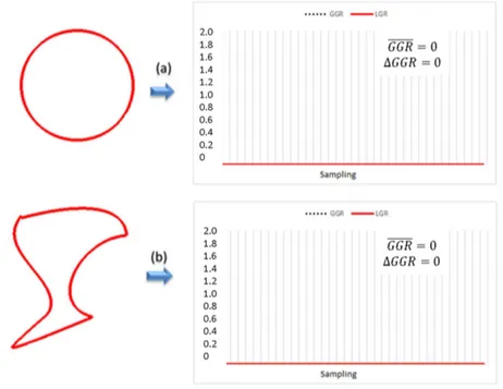
Figure 5A presents the same phantom lesions used in Figure 4, but in this case both lesions show the same growth along the border. It can be observed that GGR in both images is quite regular, and this is corroborated by ΔGGR which in both cases is less than 0.2. Although naked eye observation shows that both lesions maintained their proportions, a careful examination of ΔLGR value shows that this behavior is only found for Figure 5A-a. In fact, in Figure 5A-b the lesion has suffered deformation, this is conirmed by their ΔLGR higher than 0.2. The circularity values conirm what is visually suggested, that is the image
It
0 has a circular type shape in Figure 5A-a and a non-circular type shape in Figure 5A-b.
In Figure 5B there are two examples of lesions with abnormal cases of growth. In Figure 5B-a a non-circular type shape lesion grows into a circular
one, and in Figure 5B-b a circular type shape lesion grows into a non-circular form. It can be observed that GGR and LGR behavior in both images is quite irregular, which is conirmed by their ΔGGR and ΔLGR values above 0.2. This means that their absolute growth is irregular and their shape suffered deformation through time. Also in this case, the circularity values conirm what is visually suggested, that is image It
0 is a non-circular type shape in Figure 5B-a and a circular type shape in Figure 5B-b.
In Figure 5C there are two cases of real lesions that evolved over time, obtained from two patients in a routine dermatologist examination. It is observed that both images have variations on their growth along the border, as both ΔGGR is higher than 0.2.
Regarding the local growth, and analyzing ΔLGR, both these lesions have values above 0.2 showing a presence of deformation. Furthermore, it is clear that in Figure 5C-b we are in the presence of a substantial deformation.
Finally, in what concerns circularity of the lesion we show two cases in Figure 5C. In Figure 5C-a, even though we have the presence of small variations on the border, the shape is circular as conirmed by circularity <0.2. In Figure 5C-b we are in the presence of a non-circular type shape. These two results are consistent with the visual assessment.
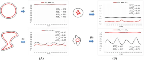
For global symmetry, this coeficient is close to 1 when the image is symmetrical or almost symmetrical
(referred to the orthonormal reference system considered). As regards the phantom evaluation, notice that the values of ACS never exceeded 1. So when the average values of ACS, represented by ACSt
0 and ACSt1, are above 0.8 (Table 1E), the image is assumed to be symmetrical, regardless of the angle of rotation of the orthonormal reference system considered. This can be observed in Figure 6A-a for
It
0 and It1, in Figure 6B-a for It1 and in Figure 6B-b for It
0. In the remaining phantom images, the lesions lack symmetry and the corresponding average values of the ACS decrease.
It is also calculated the deviation of the ACS in each case, denoted by ∆ACSt
0 and ∆ACSt1. Notice that, if the symmetry of the lesion is independent of the angle of rotation of the orthonormal reference system considered, these coeficients are closer to zero, and therefore the lesion has a circular type shape. Following Table 1F, this can be observed in Figure 6A-a for It
0 and It1, in Figure 6B-a for It1 and in Figure 6B-b for It
0. If the deviation of the ACS is higher than 0.2, as veriied in the rest of the phantoms, this means that there are some speciic positions (angles) of the orthonormal reference system considered for
which the lesion is more symmetric, and therefore it is not of a circular type.
In Figure 7 it is considered the case of two real lesions that evolved through time. When comparing the two images, it is possible to observe that Figure 7a is visually symmetrical while Figure 7b is not. That is relected on their ACS
ti, showing in Figure 7a a symmetric lesion and in Figure 7b lack of symmetry.
Finally, ∆ACS
ti is also consistent with the decision for circularity, as in Figure 7a it is presented an image with a deviation smaller than 0.2, therefore is assumed to be of a circular type shape, and in Figure 7b we have the opposite.
Discussion
Early diagnosis is important for the prognosis of melanocytic skin lesions and the measurements obtained through the proposed mathematical model increases the discriminating capability of the classical diagnosis when applied at the follow-up of the lesions. The ability to quantify the growth pattern of a certain lesion is important when accessing growing and growth rate.
The method developed proved to show very accurate information about the target growth markers (variation on the growth along the border, the deformation and the symmetry of the lesion trough the time). All the results, validated by the expected phantom outputs, were similar to the ones on the real images. Also the measurements of the circularity and the ∆ACS, which were derivate from the previous markers and both used to quantify the circular type of the shape of the lesions, not only have coincident qualitative results, but also have the expected response for all the images.
The assessment of these quantitative markers can be used to increase the eficacy of automatic classiication using machine learning algorithms. The use of growing factors and symmetry coeficients joint with texture analysis features is now being
considered and worked in our research group.
Acknowledgements
This work was partly supported by the Portuguese program CENTRO-07-ST24-FEDER-002022 / QREN. Figure 6. Symmetry factors. A: Symmetry for phantom lesions with regular absolute growth - (a) regular shaped and (b) irregular; B: Symmetry for phantom lesions with irregular absolute growth - (a) evolves from an irregular shape to one regular and (b) evolves from a regular shape to one irregular.
We have to acknowledge to Juliana Baptista MD, Dermatologist for her contribution in image acquisition.
References
Abbas Q, Celebi ME, Garcia IF, Ahmad W. Melanoma recognition framework based on expert definition of ABCD for dermoscopic images. Skin Research and Technology. 2013; 19(1):e93-102. http://dx.doi.org/10.1111/j.1600-0846.2012.00614.x. PMid:22672769.
Abbas Q, Celebi ME, Garcia IF, Rashid M. Lesion border detection in dermoscopy images using dynamic programming. Skin Research and Technology. 2011; 17(1):91-100. http:// dx.doi.org/10.1111/j.1600-0846.2010.00472.x. PMid:21226876. Afonso A, Silveira M. Hair detection in dermoscopic images using percolation. In: Proceedings of the IEEE Annual International Conference of the Engineering in Medicine and Biology Society ; 2012; San Diego, CA. IEEE; 2012. p. 4378-81.
Andreassi L, Perotti R, Rubegni P, Burroni M, Cevenini G, Biagioli M, Taddeucci P, Dell’Eva G, Barbini P. Digital dermoscopy analysis for the differentiation of atypical nevi and early melanoma: a new quantitative semiology. Archives of Dermatology. 1999; 135(12):1459-65. http:// dx.doi.org/10.1001/archderm.135.12.1459. PMid:10606050.
Argenziano G, Catricalà C, Ardigo M, Buccini P, De Simone P, Eibenschutz L, Ferrari A, Mariani G, Silipo V, Sperduti I, Zalaudek I. Seven-point checklist of dermoscopy revisited. British Journal of Dermatology. 2011; 164(4):785-90. http://dx.doi.org/10.1111/j.1365-2133.2010.10194.x. PMid:21175563.
Baumert J, Schmidt M, Giehl KA, Volkenandt M, Plewig G, Wendtner C, Schmid-Wendtner MH. Time trends in tumour thickness vary in subgroups: analysis of 6475 patients by age, tumour site and melanoma subtype. Melanoma Research. 2009; 19(1):24-30. http://dx.doi.org/10.1097/ CMR.0b013e32831c6fe7. PMid:19430403.
Benelli C, Roscetti E, Pozzo VD, Gasparini G, Cavicchini S. The dermoscopic versus the clinical diagnosis of melanoma. European Journal of Dermatology. 1999; 9(6):470-6. PMid:10491506.
Bleyer A, Viny A, Barr R. Cancer in 15- to 29-year-olds by primary site. The Oncologist. 2006; 11(6):590-601. http:// dx.doi.org/10.1634/theoncologist.11-6-590. PMid:16794238.
Blum A, Rassner G, Garbe C. Modified ABC-point list of dermoscopy: A simplified and highly accurate dermoscopic algorithm for the diagnosis of cutaneous melanocytic lesions. Journal of the American Academy of Dermatology. 2003; 48(5):672-8. http://dx.doi.org/10.1067/mjd.2003.282. PMid:12734495.
Cheng B, Joe Stanley R, Stoecker WV, Stricklin SM, Hinton KA, Nguyen TK, Rader RK, Rabinovitz HS, Oliviero M, Moss RH. Analysis of clinical and dermoscopic features for basal cell carcinoma neural network classification. Skin Research and Technology. 2013; 19(1):e217-22. http://dx.doi. org/10.1111/j.1600-0846.2012.00630.x. PMid:22724561.
Dal Pozzo V, Benelli C, Roscetti E. The seven features for melanoma: a new dermoscopic algorithm for the diagnosis of malignant melanoma. European Journal of Dermatology. 1999; 9(4):303-8. PMid:10356410.
Downing A, Newton-Bishop JA, Forman D. Recent trends in cutaneous malignant melanoma in the Yorkshire region of England; incidence, mortality and survival in relation to stage of disease, 1993-2003. British Journal of Cancer. 2006; 95(1):91-5. http://dx.doi.org/10.1038/sj.bjc.6603216. PMid:16755289.
Ferlay J, Steliarova-Foucher E, Lortet-Tieulent J, Rosso S, Coebergh JW, Comber H, Forman D, Bray F. Cancer incidence and mortality patterns in Europe: estimates for 40 countries in 2012. European Journal of Dermatology. 2013; 49(6):1374-403. PMid:23485231.
Fonseca-Pinto R, Caseiro P, Andrade A. Image Empirical Mode Decomposition (IEMD) in dermoscopic images: artefact removal and lesion border detection. In: Zagar B, Kuijper A, Sahbi H, editors. Proceedings of Signal Processing Pattern Recognition and Applications; 2010 Feb 17-19; Innsbruck, Austria. Austria: Acta Press; 2010.
Holterhues C, Vries E, Louwman MW, Koljenovic S, Nijsten T. Incidence and trends of cutaneous malignancies in the Netherlands, 1989-2005. The Journal of Investigative Dermatology. 2010; 130(7):1807-12. http://dx.doi.org/10.1038/ jid.2010.58. PMid:20336085.
Joel G, Schmid-Saugeon P, Guggisberg D, Cerottini JP, Braun R, Krischer J, Saurat JH, Murat K. Validation of segmentation techniques for digital dermoscopy. Skin Research and Technology. 2002; 8(4):240-9. http://dx.doi. org/10.1034/j.1600-0846.2002.00334.x. PMid:12423543. Liu Z, Sun J, Smith L, Smith M, Warr R. Distribution quantification on dermoscopy images for computer-assisted diagnosis of cutaneous melanomas. Medical & Biological Engineering & Computing. 2012; 50(5):503-13. http:// dx.doi.org/10.1007/s11517-012-0895-7. PMid:22438064. Longo DL, Fauci AS, Kasper DL, Hauser SL, Jameson JL, Loscalzo J. Harrison’s principles of internal medicine. 18th ed. New York: McGraw-Hill; 2012.
Mendonca T, Marcal AR, Vieira A, Nascimento JC, Silveira M, Marques JS, Rozeira J. Comparison of segmentation methods for automatic diagnosis of dermoscopy images. In: Conference Proceedings IEEE Engineering in Medicine and Biology Society; 2007 Aug 23-26; Lyon, France. Lyon: IEEE Press; 2007. p. 6573-76.
Menzies SW, Ingvar C, McCarthy WH. A sensitivity and specificity analysis of the surface microscopy features of invasive melanoma. Melanoma Research. 1996; 6(1):55-62. http://dx.doi.org/10.1097/00008390-199602000-00008. PMid:8640071.
Piccolo D, Crisman G, Schoinas S, Altamura D, Peris K. Computer-automated ABCD versus dermatologists with different degrees of experience in dermoscopy. European Journal of Dermatology. 2014; 24(4):477-81. PMid:24721784. Piccolo D, Ferrari A, Peris K, Daidone R, Ruggeri B, Chimenti S. Dermoscopic diagnosis by a trained clinician vs. a clinician with minimal dermoscopy training vs. computer-aided diagnosis of 341 pigmented skin lesions: a comparative study. British Journal of Dermatology. 2002; 147(3):481-6. http://dx.doi.org/10.1046/j.1365-2133.2002.04978.x. PMid:12207587.
Rogers HW, Weinstock MA, Harris AR, Hinckley MR, Feldman SR, Fleischer AB, Coldiron BM. Incidence estimate of nonmelanoma skin cancer in the United States, 2006. Archives of Dermatology. 2010; 146(3):283-7. http:// dx.doi.org/10.1001/archdermatol.2010.19. PMid:20231499.
Sadri AR, Zekri M, Sadri S, Gheissari N, Mokhtari M, Kolahdouzan F. Segmentation of dermoscopy images using wavelet networks. IEEE Transactions on Biomedical Engineering. 2013; 60(4):1134-41. http://dx.doi.org/10.1109/ TBME.2012.2227478. PMid:23193305.
Sant M, Allemani C, Santaquilani M, Knijn A, Marchesi F, Capocaccia R. EUROCARE-4. Survival of cancer patients diagnosed in 1995-1999. Results and commentary. European Journal of Cancer. 2009; 45(6):931-91. http:// dx.doi.org/10.1016/j.ejca.2008.11.018. PMid:19171476. Şavk E, Şahinkarakaş E, Okyay P, Karaman G, Erkek M, Şendur N. Interobserver agreement in the use of the ABCD rule for dermoscopy. The Journal of Dermatology. 2004; 31(12):1041-3. http://dx.doi.org/10.1111/j.1346-8138.2004. tb00652.x. PMid:15801273.
Skender-Kalnenas TM, English DR, Heenan PJ. Benign melanocytic lesions: risk markers or precursors of cutaneous melanoma? Journal of the American Academy of Dermatology. 1995; 33(6):1000-7. http://dx.doi.org/10.1016/0190-9622(95)90294-5. PMid:7490345.
Soyer HP, Kerl H. Surface microscopy of pigmented cutaneous tumors. Annales de Dermatologie et de Venereologie. 1993; 120(1):15-20. PMid:8338324.
Soyer HP, Smolle J, Leitinger G, Rieger E, Kerl H. Diagnostic reliability of dermoscopic criteria for detecting malignant melanoma. Dermatology (Basel, Switzerland). 1995; 190(1):25-30. http://dx.doi.org/10.1159/000246629. PMid:7894091.
Stern RS. Prevalence of a history of skin cancer in 2007: Results of an incidence-based model. Archives of Dermatology. 2010; 146(3):279-82. http://dx.doi.org/10.1001/ archdermatol.2010.4. PMid:20231498.
Toossi MT, Pourreza HR, Zare H, Sigari MH, Layegh P, Azimi A. An effective hair removal algorithm for dermoscopy images. Skin Research and Technology. 2013; 19(3):230-5. http://dx.doi.org/10.1111/srt.120119(3):230-5. PMid:23560826.
Tryggvadóttir L, Gislum M, Hakulinen T, Klint A, Engholm G, Storm HH, Bray F. Trends in the survival of patients diagnosed with malignant melanoma of the skin in the Nordic countries 1964-2003 followed up to the end of 2006. Acta Oncologica. 2010; 49(5):665-72. http://dx.doi. org/10.3109/02841861003702528. PMid:20491525. Wang H, Chen X, Moss RH, Stanley RJ, Stoecker WV, Celebi ME, Szalapski TM, Malters JM, Grichnik JM, Marghoob AA, Rabinovitz HS, Menzies SW. Watershed segmentation of dermoscopy images using a watershed technique. Skin Research and Technology. 2010; 16(3):378-84. PMid:20637008.
Whiteman DC, Pavan WJ, Bastian BC. The melanomas: a synthesis of epidemiological, clinical, histopathological, genetic, and biological aspects, supporting distinct subtypes, causal pathways, and cells of origin. Pigment Cell & Melanoma Research. 2011; 24(5):879-97. http://dx.doi. org/10.1111/j.1755-148X.2011.00880.x. PMid:21707960. Zalaudek I, Argenziano G, Soyer HP, Corona R, Sera F, Blum A, Braun RP, Cabo H, Ferrara G, Kopf AW, Langford D, Menzies SW, Pellacani G, Peris K, Seidenari S. Three-point checklist of dermoscopy: an open internet study. British Journal of Dermatology. 2006a; 154(3):431-7. http://dx.doi. org/10.1111/j.1365-2133.2005.06983.x. PMid:16445771. Zalaudek I, Leinweber B, Hofmann-Wellenhof R, Soyer HP. The impact of dermoscopic-pathologic correlates in the diagnosis and management of pigmented skin tumors. Expert Review of Dermatology. 2006b; 1(4):579-87. http:// dx.doi.org/10.1586/17469872.1.4.579.
Zalaudek I, Kreusch J, Giacomel J, Ferrara G, Catricala C, Argenziano G. How to diagnose nonpigmented skin tumors: a review of vascular structures seen with dermoscopy: part I. Melanocytic skin tumors. Journal of the American Academy of Dermatology. 2010; 63(3):361-74, quiz 375-6. http:// dx.doi.org/10.1016/j.jaad.2009.11.698. PMid:20708469.
Authors
Ana Isabel Mendes1*, Conceição Nogueira1, Jorge Pereira2, Rui Fonseca-Pinto1,2
1 Department of Mathematics, School of Technology and Management, Instituto Politécnico de Leiria, Campus 2,
Apartado 4163, CEP 2411-901, Leiria, Portugal.