Differential Evolution Enhanced with Eager Random Search for Solving Real-Parameter Optimization Problems

(1)

Differential Evolution Enhanced with Eager Random

Search for Solving Real-Parameter Optimization

Problems

Miguel

Leon

Schoolof Innovation,Design andEgineering MalardalenUniversity

Vasteras, Sweden

Ning

Xiong

Schoolof Innovation,DesignandEgineering Malardalen University

Vasteras,Sweden

Abstract—Differential evolution (DE) presents a class of evo-lutionary computing techniques that appear effective to handle real parameter optimization tasks in many practical applications. However, the performance of DE is not always perfect to ensure fast convergence to the global optimum. It can easily get stagnation resulting in low precision of acquired results or even failure. This paper proposes a new memetic DE algorithm by incorporating Eager Random Search (ERS) to enhance the performance of a basic DE algorithm. ERS is a local search method that is eager to replace the current solution by a better candidate in the neighborhood. Three concrete local search strategies for ERS are further introduced and discussed, leading to variants of the proposed memetic DE algorithm. In addition, only a small subset of randomly selected variables is used in each step of the local search for randomly deciding the next trial solution. The results of tests on a set of benchmark problems have demonstrated that the hybridization of DE with Eager Random Search can substantially augment DE algorithms to find better or more precise solutions while not requiring extra computing resources.

Keywords—Evolutionary Algorithm, Differential Evolution, Ea-ger Random Search, Memetic Algorithm, Optimization

I. INTRODUCTION

Evolutionary algorithms (EAs) are stochastic and bio-logically inspired techniques that provide powerful and ro-bust means to solve many real-world optimization problems. They are population-based optimization approaches [1] which perform parallel and beam search, thereby exhibiting strong global search ability in complex and high dimensional spaces. Another merit of EAs is that they dont need the derivative information of objective functions. This is very attractive for wide applications of EAs in various situations without requir-ing the problem space to be continuous and differentiable. Many variants of EAs have been developed to deal with real-parameter continuous optimization problems, including evolution strategies [2], real-coded genetic algorithms [3], [4], differential evolution (DE) [5], [6], and particle swarm optimization [7] and [8].

Differential evolution presents a class of evolutionary techniques to solve real parameter optimization tasks with nonlinear and multimodal objective functions. Despite sharing common concepts of EAs, DE differs from many other EAs in that mutation in DE is based on differences of pair(s)

of individuals randomly selected from the population. Thus, the direction and magnitude of the search is decided by the distribution of solutions instead of a pre-specified probability density function. DE has been used as very competitive al-ternative in many practical applications due to its simple and compact structure, easy use with fewer control parameters, as well as high convergence in large problem spaces. However, the performance of DE is not always excellent to ensure fast convergence to the global optimum. It can easily get stagnation resulting in low precision of acquired results or even failure [9].

Recent researches have shown that hybridization of EAs with other techniques such as metaheuristics or local search techniques can greatly improve the efficiency of the search. EAs that are augmented with local search for self-refinement are called Memetic Algorithms (MAs) [[10], [11]]. In MAs, a local search mechanism is applied to members of the population in order to exploit the most promising regions gath-ered from global sampling done in the evolutionary process. Memetic computing has been used with DE to refine individ-uals in their neighborhood. Norman and Iba [12] proposed a crossover-based adaptive method to generate offspring in the vicinity of parents. Many other works apply local search mechanisms to certain individuals of every generation to obtain possibly even better solutions, see examples in ([13], [14], [15], [16]), [17]).

This paper proposes a new memetic DE algorithm by incorporating Eager Random Search (ERS) to enhance the performance of a conventional DE algorithm. ERS is a local search method that is eager to move to a position that is identified as better than the current one without considering other opportunities in the neighborhood. This is different from common local search methods such as gradient descent [18] or hill climbing [19] which seek local optimal actions during the search. Forsaking optimality of moves in ERS is advantageous to increase randomness and diversity of search for avoiding premature convergence. Three concrete local search strategies within ERS are introduced and discussed, leading to variants of the proposed memetic DE algorithm. In addition, only a small subset of randomly selected variables is used in every step of the local search for randomly deciding the next trial point. The results of tests on a set of benchmark problems have demonstrated that the hybridization of DE with

(2)

Eager Random Search can bring improvement of performance compared to pure DE algorithms while not incurring extra computing expenses.

The rest of the paper is organized as follows. Section 2 briefly presents the related works. Section 3 introduces the basic DE algorithm. Then, the proposed memetic DE algorithm in combination with Eager Random Search is presented in details in Section 4. Section 5 gives the results of tests for evaluation. Finally, concluding remarks are given in Section 6.

II. RELATEDWORK

Since the first proposal of DE in 1997 [20], a lot of works have been done to improve the search ability of this algorithm, resulting in many variants of DE. A brief overview on some of them is given in this section.

Ali, Pant and Nagar [13] proposed two different local search algorithms, namely Trigonometric Local Search and Interpolated Local Search, which were applied to refine the best solution and two random solutions in every generation respectively.

Local search differential evolution was developed in [14] where a new local search operator was used on every individual in the population with a probability. The search strategy attempted to find a random better solution between trial vector and the best solution in the generation.

Dai, Zhou, Zhang and Jiang [15] combined Orthogonal Local Search with DE in the so-called OLSDE (Orthogonal Local Search Differential Evolution) algorithm. Therein two individuals were randomly selected from the population in each generation and they were used to generate a group of trial solutions with the orthogonal method. Then the best solution from the group of trial solutions replaced the worst individual in the population.

Jia, Zheng and Khan [9] proposed a memetic DE algorithm in combination with chaotic local search (CLS). The adaptive shrinking strategy embedded within CLS enabled the DE optimizer to explore large space in the early search phase and to exploit small regions in the later phase. Moreover, the chaotic iteration produced a higher probability to move into a boundary field, which appeared helpful for avoiding premature convergence to some extent. A similar work of utilizing chaotic principle based local search in DE was presented in [21].

Poikolainen and Neri [22] proposed a DE algorithm em-ploying concurrent fitness based local search (DEcfbLS). The local search was applied to multiple promising solutions in the population, and the selection of individuals for local improvement was based on a fitness-based adaptation rule. Further, the local search operator was realized by making trial moves successively on single dimensions. But there was not much variation in the step sizes of the moves for different variables within an iteration of the search.

III. BASICDE

DE is a stochastic and population based algorithm with Np individuals in the population. Every individual in the population stands for a possible solution to the problem. One of the Np individuals is represented byXi,gwithi= 1,2, ., Np

andgis the index of the generation. DE has three consecutive steps in every iteration: mutation, recombination and selection. The explanation of these steps is given below:

MUTATION. Np mutated individuals are generated using some individuals of the population. The vector for the mutated solution is called mutant vector and it is represented byVi,g. There are some ways to mutate the current population, but only three will be explained in this paper. The notation to name them isDE/x/y/z, wherexstands for the vector to be mutated, y represents the number of difference vectors used in the mutation and z stands for the crossover used in the algorithm. We will not includez in the notation because only the binomial crossover method is used here. The three mutation strategies (random, current to best and current to rand) will be explained below. The other mutation strategies and their performance are given in [23].

- Random Mutation Strategy:

Random mutation strategy attempts to mutate three indi-vidual in the population. When only one difference vector is employed in mutation, the approach is represented by DE/rand/1. A new, mutated vector is created according to Eq. 1

Vi,g=Xr1,g+F×(Xr2,g−Xr3,g) (1)

where Vi,g represents the mutant vector, i stands for the index of the vector,g stands for the generation,r1, r2, r3∈ {

1,2,. . . ,Np} are random integers andF is the scaling factor in the interval [0, 2].

Fig. 1 shows how this mutation strategy works. All the variables in the figure appear in Eq. 1 with the same meaning, anddis the difference vector between Xr2,g and Xr3,g.

Fig. 1: Random mutation strategy

- Current to Best Mutation Strategy:

The current to best mutation strategy is referred as DE/current-to-best/1. It moves the current individual towards the best individual in the population before being disturbed

(3)

with a scaled difference of two randomly selected vectors. Hence the mutant vector is created by

Vi,g=Xi,g+F1×(Xbest,g−Xi,g)+F2×(Xr1,g−Xr2,g) (2)

where Vi,g stands for the mutant vector, Xi,g and Xbest,g represent the current individual and the best individual in the population respectively, F1 andF2 are the scaling factors in the interval [0, 2] and r1, r2 ∈ { 1,2,. . . ,Np} are randomly created integers.

Fig. 2 shows how the DE/current-to-best/1 strategy works to produce a mutant vector, where d1 denotes the difference vector between the current individualXi,g, and Xbest,g,d2 is the difference vector between Xr1,g andXr2,g.

Fig. 2: Current to best mutation strategy

- Current to Rand Mutation Strategy:

The current to rand mutation strategy is referred to as DE/current-to-rand/1. It moves the current individual towards a random vector before being disturbed with a scaled difference of two randomly selected individuals. Thus the mutant vector is created according to Eq. 3 as follows

Vi,g=Xi,g+F1×(Xr1,g−Xi,g)+F2×(Xr2,g−Xr3,g) (3)

whereXi,grepresents the current individual,Vi,gstands for the mutant vector,gstands for the generation,iis the index of the vector,F1andF2are the scaling factors in the interval [0, 2] andr1, r2, r3∈ {1,2,. . . ,Np} are randomly created integers.

Fig. 3 explains how the DE/current-to-rand/1 strategy works to produce a mutant vector, where d1is the difference vector between the current individual,Xi,g, andXr1,g, andd2

is the difference vector between Xr3,g andXr2,g.

CROSSOVER. In step two we recombine the set of mutated solutions created in step 1 (mutation) with the original popu-lation members to produce trial solutions. A new trial vector is denoted byTi,gwhereiis the index andgis the generation.

Fig. 3: Current to rand mutation strategy

Every parameter in the trial vector is calculated with equation 3

Ti,g[j] = _V

i,g[j] ifrand[0,1]< CR or j=jrand Xi,g[j] otherwise

(4)

wherejstands for the index of every parameter in a vector, CR is the probability of the recombination andjrandis a randomly selected integer in[1, Np]to ensure that at least one parameter from the mutant vector is selected.

SELECTION. In this last step we compare a trial vector with its parent in the population with the same index i to choose the stronger one to enter the next generation Therefore, if the problem to solve is a minimization problem, the next generation is created according to equation 4

Xi,g+1=

Ti,g if f(Ti,g)< f(Xi,g) Xi,g otherwise

(5)

where Xi,g is an individual in the population, Xi,g+1 is the

individual in the next generation,Ti,gis the trial vector,f(Ti,g) stands for the fitness value of trial solution andf(Xi,g)is the fitness value of the individual in the population.

The pseudocode for basic DE is given in Alg. 1. First of all we create the initial population with randomly generated individuals. Then we evaluate every individual in the popula-tion with a fitness funcpopula-tion. Afterward we perform the three main steps: mutation, recombination and selection. First we mutate the population according Eq. 1, Eq. 2 or Eq. 3, then we recombine mutant vectors and their parents to get trial vectors according to Eq. 4, which are also called offspring. Finally we compare the offspring with their parents and the better individuals get into the updated population. From step 3 to step 7 we need to repeat it until the termination condition is satisfied.

(4)

Algorithm 1 Differential Evolution

1: Initialize the population with ramdomly created individu-als

2: Calculate the fitness values of all individuals in the popu-lation

3: while The termination condition is not satisfieddo 4: Create mutant vectors using a mutation strategy in Eq.

1, Eq. 2 or Eq. 3

5: Create trial vectors by recombining mutant vectors with parents vector according to Eq. 4

6: Evaluate trial vectors with their fitness function 7: Select winning vectors according to Eq. 5 as individuals

in the next generation 8: end while

IV. DE INTEGRATED WITHERS

This section is devoted to the proposal of the memetic DE algorithm with integrated ERS for local search. We will first introduce ERS as a general local search method together with its three concrete (search) strategies, and then we shall outline how ERS can be incorporated into DE to enable self-refinement of individuals inside a DE process.

A. Eager Random Local Search (ERS)

The main idea of ERS is to immediately move to a randomly created new position in the neighborhood without considering other opportunities as long as this new position receives a better fitness score than the current position. This is different from some other conventional local search methods such as Hill Climbing in which the next move is always to the best position in the surroundings. Forsaking optimality of moves in ERS is beneficial to achieve more randomness and diversity of search for avoiding local optima. Further, in exploiting the neighborhood, only a small subset of randomly selected variables undergoes changes to randomly create a trial solution. If this trial solution is better, it simply replaces the current one. Otherwise a new trial solution is generated with other randomly selected variables. This procedure is terminated when a given number of trial solutions have been created without finding improved ones. The formal procedure of ERS is given in Algorithm 2, whereαdenotes the portion of variables that are subject to local changes and M is the maximum number of times a trial solution can be created in order to find a better position than the current one.

The next more detailed issue with ERS is how to change a selected variable in making a trial solution in the neighbor-hood. This corresponds to the way to assign a possible value for parameter k in line 7 of Algorithm 2. Our idea is to solve this issue using a suitable probability function. We consider three probability distributions (uniform, normal, and Cauchy) as alternatives for usage when generating a new value for a selected parameter/variable. The use of different probability distributions lead to different local search strategies within the ERS family, which will be explained in the sequel.

1) Random Local Search (RLS): In Random Local Search

(RLS), we simply use a uniform probability distribution when new trial solutions are created given a current solution. To be more specific, when dimension k is selected for change, the

Algorithm 2 Eager Random Local Search

1: Seti = 1;

2: while i <=M do

3: candidates= 1,2,. . . ,dimension; 4: Setj = 1;

5: while j < α∗dimension do 6: Randomly selectkfrom candidates;

7: Assign a random possible value to parameterkof the vector;

8: Removek fromcandidates; 9: Setj = j + 1;

10: end while

11: ifThis new solution is better than the parent then 12: Replace the parent solution with the new one; 13: Seti= 1;

14: else

15: Seti= i + 1; 16: end if

17: end while

trial solutionX′_{will get the following value on this dimension} regardless of its initial value in the current solution:

X′[k] =rand(ai, bi) (6) where rand(ai, bi) is a uniform random number between ai andbi , and ai andbi are the minimum and maximum values respectively on dimension k.

As equal chance is given to the whole range of a variable when changing a solution, RLS is more likely to create new points with large variation, thus increasing the opportunity to jump out from a local optimum. The disadvantage of RLS lies on its fine tuning ability to reach the exact optimum.

2) Normal Local Search (NLS): In Normal Local Search

(NLS), we create a new trial solution by disturbing the current solution in terms of a normal probability distribution. This means that, if dimension k is selected for change, the value on this dimension for trial solutionX′ will be given by

X′[k] =X[k] +N(0, δ) (7) whereN(0, δ)represents a random number generated accord-ing to a normal density function with its mean beaccord-ing zero.

Owing to the use of the normal probability distribution, NLS usually creates new trial solutions that are quite close to the current one. This may, on one hand, bring benefit for the fine-tuning ability to reach the exact optimum. But, on the other hand, it will make it more difficult for the local search to escape from a local optimum.

3) Cauchy Local Search (CLS): In this third local search

strategy, we apply the Cauchy density function in creating trial solutions in the neighborhood. It is called Cauchy Local search (CLS). A nice property of the Cauchy function is that it is centered around its mean value whereas exhibiting a wider distribution than the normal probability function, as is shown in Fig. 3. Hence CLS will have more chances to make big moves in attempts to find possibly better positions and to leave away

(5)

from local minima. Regarding the fine-search ability, CLS will be better than RLS though it is not expected as good as NLS.

More concretely, a Cauchy probability density function is defined by

f(x) = 1

π× t

t2₊_x2, t >0 (8)

Its corresponding cumulative probability function is given by

F(x) =1 2 +

1

π×arctan( x

t) (9)

It follows that, on a selected dimensionk, the value of trial solution X′ _{will be generated as follows:}

X′[k] =X[k] +t×tan(π×(rand(0,1)−0.5)) (10)

whererand(0,1)is a random uniform number between 0 and 1.

Fig. 4: Distribution probability

B. The Proposed Memetic DE Algorithm

Here with we propose a new memetic DE algorithm by combining basic DE with Eager Random Search (ERS). ERS is applied in each generation after completing the mutation, crossover and selection operators. The best individual in the population is used as the starting point when ERS is executed. If ERS terminates with a better solution, it is inserted into the population and the current best member in the population is discarded. The general procedure of the proposed memetic DE algorithm is outlined in Algorithm 3.

Finally, different strategies within ERS can be used for local search in line 9 of Algorithm 3. We use DERLS, DENLS, and DECLS to refer to the variants of the proposed memetic DE algorithm that adopt RLS, NLS, and CLS respectively as local search strategies.

Algorithm 3 Memetic Differential Evolution

1: Initialize the population with randomly created individuals 2: Calculate the fitness values of all individuals in the

popu-lation

3: while The termination condition is not satisfieddo 4: Create mutant vectors using a mutation strategy in Eq.

1, Eq. 2 or Eq. 3

5: Create trial vectors by recombining mutant vectors with parents vector according to Eq. 4

6: Evaluate trial vectors with their fitness function 7: Select winning vectors according to Eq. 5 as individuals

in the next generation

8: Identify the best individualXbest in the population 9: Perform local search fromXbest using a ERS strategy 10: if the result from local search Xr is better than Xbest

then

11: replaceXbest byXr in the population 12: end if

13: end while

V. EXPERIMENTS ANDRESULTS

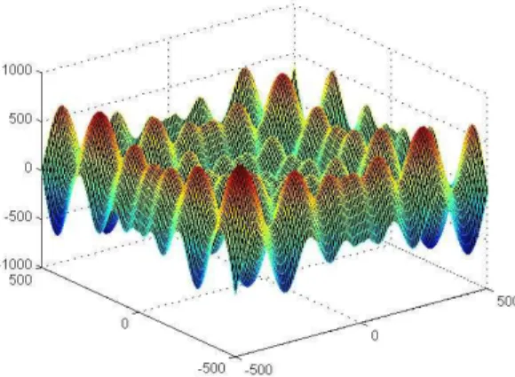
To examine the merit our proposed memetic DE algorithm compared to basic DE, we tested the algorithms in thirteen benchmark functions [24] listed in Table 1. Functions 1 to 7 are unimodal and functions 8 to 13 are multimodal functions that contain many local optima. Table 1 gives the definition of every function. The most difficult functions are 8, 9 and 10, which are shown in Figs. 5, 6 and 7 respectively.

Fig. 5: Function 8 with two dimensions

A. Experimental Settings

DE has three main control parameters: population size (Np), crossover rate (CR) and the scaling factor (F) for mutation. The following specification of these parameters was used in the experiments: N p = 60, CR = 0.85 and F, F1, F2 = 0.9. All the algorithms were applied to the benchmark problems with the aim to find the best solution for each of them. Every algorithm was executed 30 times on every function to acquire a fair result for the comparison. The condition to finish the execution of DE programs is that the error of the best result found is below 10e-8 with respect to the true minimum or the number of evaluations has exceeded

(6)

TABLE I: The thirteen functions used in the experiments

FUNCTION

f1(x) =Pn i=1x

2

i f2(x) =Pn

i=1|xi|+

Qn i=1|xi|

f3(x) =Pn i=1(

Pi j=1xj)

2

f4(x) =maxi{|xi|,1≤i≤n} f5(x) =Pn−1

i=1[100×(xi+1−x 2

i)

2

+ (xi−1)

2

]

f6(x) =Pn i=1

(xi+ 0.5)2

f7(x) =Pn i=1i×x

4

i+random[0,1) f8(x) =Pn

i=1−xi×sin(

p |xi|)

f9(x) =Pn i=1[x

2

i−10×cos(2×π×xi) + 10] f10(x) =−20×exp(−0.2×p1

n× Pn

i=1x 2

i)−exp(

1

n× Pn

i=1cos(2πxi)) + 20 +e

f11(x) = 1 4000×

Pn i=1x

2

i− Qn

i=1cos(

xi √

i) + 1 f12(x) =π

n× {10sin

2

(πyi) + Pn−1

i=1((yi−1) 2

[1 + 10sin2(πyi+1)]) + (yn−1)2}+

+Pn

i=1u(xi,10,100,4), whereyi= 1 + 1 4(xi+ 1)

u(xi, a, k, m) = (

k(xi−a)m, xi> a

0, −a≤xi≤a k(xi−a)m, xi<−a f13(x) =0.1× {sin2(3πx1) +Pn−

1

i=1((xi−1) 2

[1 +sin2(3πxi+1)])+

+(xn−1)[1 +sin(2πxn)2]}+ Pn

i=1u(xi,5,100,4)

300,000. The parameters in DECLS are t= 0.2,M = 5and α= 0.1.

The results of experiments will be presented as follows: First we will compare the performance (the quality of acquired solutions) of the various DE approaches with random mutation strategy, secondly we will compare the performance of the same approaches using the current to rand mutation strategy and third we will compare the performance of the same approaches using the current to best mutation strategy.

B. Performance of the Memetic DE with random mutation strategy

First, random mutation strategy (DE/rand/1) was used in all DE approaches to study the effect of the ERS local search strategies in the memetic DE algorithm. The results can be observed in Table 2 and the values in boldface represent the lowest average error found by the approaches.

In Table 3 there is a ranking among all the approaches for every function. The last row represents the average of the rankings.

We can see in Table 2 and Table 3 that DECLS is the best in all the unimodal functions except on Function 4 that is the second best. In multimodal functions, DERLS is the best on Functions 8, 10 and 11. DECLS found the exact optimum all the times in Functions 12 and 13. The basic, DE performed the worst in multimodal functions. According to the above analysis, we can say that DECLS improve a lot the performance of basic DE with random mutation strategy and also we found out that DERLS is really good in multimodal functions particularly on Function 8, which is the most difficult function. Considering all the functions and the average ranking in Table 3, the best algorithm is DECLS and the weakest one is the basic DE.

(7)

TABLE II: Average error of the found solutions on the test problems with random mutation strategy

FUNC. DE DERLS DENLS DECLS f1 0,00E+00 0,00E+00 0,00E+00 0,00E+00

(4,56E-14) (6,80E-13) (1,21E-13) (1,33E-14) f2 1,82E-08 5,30E-08 2,26E-08 1,42E-08

(1,13E-08) (2,39E-08) (1,32E-08) (1,07E-08) f3 6,55E+01 8,01E+01 1,11E+00 6,54E-01

(3,92E+01) (4,88E+01) (1,10E+00) (1,47E+01) f4 6,22E+00 2,37E+00 1,80E-02 5,66E-01

(5,07E+00) (1,87E+00) (7,28E-01) (3,68E-01) f5 2,31E+01 2,27E+01 2,65E+01 2,03E+01

(2,00E+01) (1,81E+01) (2,41E+01) (2,62E+01) f6 0,00E+00 0,00E+00 0,00E+00 0,00E+00

(0,00E+00) (0,00E+00) (0,00E+00) (0,00E+00) f7 1,20E-01 1,15E-02 1,23E-02 1,05E-02

(3,79E-03) (3,16E-03) (3,29E-03) (3,61E-03) f8 2,72E+03 2,31E+02 1,86E+03 1,58E+03

(8,15E+02) (1,50E+02) (5,46E+02) (5,16E+02) f9 1,30E+01 1,28E+01 6,17E+00 7,72E+00

(3,70E+00) (3,72E+00) (2,06E+00) (2,43E+00) f10 1,88E+01 1,87E+00 4,94E+00 5,50E+00

(4,28E+00) (4,76E+00) (8,11E+00) (7,53E+00) f11 8,22E-04 8,22E-04 1,49E-02 1,44E-02

(2,49E-03) (2,49E-03) (2,44E-02) (2,70E-02) f12 3,46E-03 3,46E-03 1,04E-02 0,00E+00

(1,86E-02) (1,86E-02) (3,11E-02) (8,49E-15) f13 3,66E-04 0,00E+00 0,00E+00 0,00E+00

(1,97E-03) (2,14E-13) (1,31E-14) (3,37E-15)

TABLE III: Ranking of all DE approaches with random mutation strategy

FUNCTION DE DERLS DENLS DECLS

f1 2,5 2,5 2,5 2,5

f2 2 4 3 1

f3 3 4 2 1

f4 4 3 1 2

f5 3 2 4 1

f6 2,5 2,5 2,5 2,5

f7 3 2 4 1

f8 4 1 3 2

f9 4 3 1 2

f10 4 1 2 3

f11 1,5 1,5 4 3

f12 2,5 2,5 4 1

f13 4 2 2 2

average 3,076923 2,384615 2,692308 1,846154

C. Performance of the Memetic DE with Current to Rand Mutation Strategy

The next mutation strategy used in our experiments was current to rand mutation strategy (DE/current-to-rand/1) and the results are illustrated in Table 4. The first column of this table shows the functions that we used for testing and the results for every algorithm are given in Columns 2-5.

Table 5 shows the ranking of all the approaches for every test function with current to rand mutation strategy.

We can see in Table 4 and Table 5 that in unimodal functions the best algorithm is DECLS except in Function 3 DENLS is the best. In multimodal functions, basic DE is the worst, because it has the worst results in Functions 8 and 10, two of the most difficult functions and basic DE did not find good result in Function 9. The best algorithms in multimodal functions are DECLS and DERLS. According to this analysis we can say that DECLS is most desirable as it appeared to be competent in all functions, also in the average ranking DECLS gets the best result.

TABLE IV: Average error of the found solutions on the test problems with current to rand mutation strategy

(1,20E-16) (5,50E-15) (2,53E-16) (5,23E-17) f2 0,00E+00 0,00E+00 0,00E+00 0,00E+00

(6,79E-10) (2,68E-09) (1,65E-09) (8,09E-10) f3 1,96E+01 1,99E+01 3,89E-01 4,46E-01

(9,93E+00) (1,16E+01) (2,94E-01) (3,29E-01) f4 3,30E+00 1,39E+00 6,19E-01 9,44E-02

(2,81E+00) (1,66E+00) (1,64E+00) (2,14E-01) f5 1,57E+01 1,91E+01 2,70E+01 1,49E+01

(1,48E+01) (1,82E+01) (2,70E+01) (1,94E+01) f6 0,00E+00 0,00E+00 0,00E+00 0,00E+00

(0,00E+00) (0,00E+00) (0,00E+00) (0,00E+00) f7 9,64E-03 9,36E-03 9,57E-03 9,04E-03

(9,93E-03) (2,63E-03) (2,21E-03) (3,22E-03) f8 6,71E+03 1,20E+03 5,17E+03 4,02E+03

(2,93E+02) (2,78E+02) (6,33E+02) (6,01E+02) f9 1,08E+01 1,37E+01 1,04E+01 1,01E+01

(2,39E+00) (4,45E+00) (3,72E+00) (3,41E+00) f10 1,93E+01 4,62E-01 6,92E+00 1,59E+00

(3,58E+00) (2,49E+00) (9,22E+00) (4,86E+00) f11 2,47E-04 4,93E-04 9,04E-03 3,77E-03

(1,33E-03) (1,84E-03) (2,09E-02) (7,87E-03) f12 0,00E+00 0,00E+00 3,46E-03 0,00E+00

(1,61E-17) (5,02E-17) (1,86E-02) (9,99E-18) f13 0,00E+00 0,00E+00 0,00E+00 0,00E+00

(1,85E-13) (1,68E-11) (2,48E-12) (6,99E-15)

TABLE V: Ranking of all approaches with current to rand mutation strategy

f1 2,5 2,5 2,5 2,5

f2 2,5 2,5 2,5 2,5

f3 3 4 1 2

f4 4 3 2 1

f5 2 3 4 1

f6 3 4 2 1

f7 2 4 3 1

f8 3,5 1 3,5 2

f9 4 3 2 1

f10 4 1 3 2

f11 1 2 4 3

f12 2 2 4 2

f13 2,5 2,5 2,5 2,5

average 2,846152 2,461538 2,769231 1,923077

D. Performance of the Memetic DE with Current to Best Mutation Strategy

The last experiments were related with current to best mu-tation strategy (DE/current-to-best/1). This mumu-tation strategy was used in all DE approaches to study the effect of our proposed ERS strategies in the memetic DE algorithm. The results can be observed in Table 6 and the values in boldface represent the lowest average error found by the approaches.

In Table 7 there is a ranking among all the approaches for every function. The last row represents the average of the rankings.

We can see in Table 6 and Table 7 that DECLS got the best results in most unimodal functions. DERLS is the best on Functions 8 and 10, always finding the true optimum in Function 10. DECLS is the best algorithm in Function 9 and only this algorithm always found the true optimum in Functions 12 and 13. According to the above analysis, we can say that DECLS is the best algorithm, because it is competitive in almost all unimodal and multimodal functions. DECLS also

(8)

TABLE VI: Average error of the found solutions on the test problems with current to best mutation strategy

(1,81E-34) (8,64E-32) (1,14E-33) (1,04E-33) f2 0,00E+00 0,00E+00 0,00E+00 0,00E+00

(9,16E-20) (5,69E-19) (7,19E-19) (3,02E-19) f3 2,73E-03 7,27E-03 5,97E-02 5,09E-03

(2,57E-03) (8,06E-03) (3,21E-01) (2,64E-02) f4 6,42E-04 2,69E-03 2,98E-04 1,86E-04

(5,95E-04) (4,72E-03) (2,47E-04) (1,93E-04) f5 4,10E-01 4,34E-01 1,97E+00 1,07E+00

(1,19E+00) (1,23E+00) (3,64E+00) (1,75E+00) f6 2,33E-01 2,67E-01 6,67E-02 0,00E+00

(4,23E-01) (5,12E-01) (2,49E-01) (0,00E+00) f7 7,94E-03 8,54E-03 8,33E-03 7,77E-03

(2,45E-03) (2,21E-03) (3,40E-03) (2,40E-03) f8 2,35E+03 3,10E+02 2,35E+03 2,10E+03

(8,66E+02) (1,86E+02) (5,85E+02) (5,75E+02) f9 2,18E+01 2,02E+01 1,23E+01 1,08E+01

(4,47E+00) (5,13E+00) (6,08E+00) (3,72E+00) f10 1,06E+01 0,00E+00 2,78E+00 1,99E+00

(9,89E+00) (1,28E-15) (6,44E+00) (5,87E+00) f11 4,76E-03 9,52E-03 1,16E-01 1,01E-01

(5,28E-03) (8,59E-03) (8,04E-02) (6,79E-02) f12 2,76E-02 1,04E-02 1,42E-01 0,00E+00

(5,31E-02) (3,11E-02) (3,21E-01) (8,22E-33) f13 1,83E-03 3,66E-04 4,36E-04 0,00E+00

(4,09E-03) (1,97E-03) (1,64E-03) (2,57E-09)

TABLE VII: Ranking of all DE approaches with random mutation strategy

f1 2,5 2,5 2,5 2,5

f2 2,5 2,5 2,5 2,5

f3 1 3 4 2

f4 3 4 2 1

f5 1 2 4 3

f6 3 4 2 1

f7 2 4 3 1

f8 3,5 1 3,5 2

f9 4 3 2 1

f10 4 1 3 2

f11 1 2 4 3

f12 3 2 4 1

f13 4 3 3 1

average 2,653846 2,538462 3,038462 1,769231

gets the best ranking among others. Besides, DERLS is shown to be competitive in multimodal functions.

VI. CONCLUSIONS

In this paper we propose a memetic DE algorithm by incorporating Eager Random Search (ERS) as a local search method to enhance the search ability of a pure DE algorithm. Three concrete local search strategies (RLS, NLS, and CLS) are introduced and explained as instances of the general ERS method. The use of different local search strategies from the ERS family leads to variants of the proposed memetic DE algo-rithm, which are abbreviated as DERLS, DENLS and DECLS respectively. The results of the experiments have demonstrated that the overall ranking of DECLS is superior to the ranking of basic DE and other memetic DE variants considering all the test functions and various mutation strategies used. In addition, we found out that DERLS is much better than the other counterparts in very difficult multimodal functions.

In future work, we intend to improve our proposed algo-rithms with adaptive parameters in mutation, crossover and

local search and attempting to hybridize both alternatives to take advantage of the best features from each of them. Moreover, we will also apply and test our new computing algorithms in real industrial scenarios.

ACKNOWLEDGMENT

The work is funded by the Swedish Knowledge Foundation (KKS) grant (project no 16317). The authors are also grateful to ABB FACTS, Prevas and VOITH for their co-financing of the project. The work is also partly supported by ESS-H profile funded by the Swedish Knowledge Foundation.

REFERENCES

[1] N. Xiong, D. Molina, M. Leon, and F. Herrera, “A walk into meta-heuristics for engineering optimization: Principles, methods, and recent trends,”International Journal of Computational Intelligence Systems, vol. 8, no. 4, pp. 606–636, 2015.

[2] N. Hansen and A. Ostermeier, “Completely derandomized self-adaptation in evolution strategies,” Evolutionary Computation, vol. 9, no. 2, pp. 159–195, 2001.

[3] F. Herrera and M. Lozano, “Two-loop real-coded genetic algorithms with adaptive control of mutation step size,” Applied Intelligence, vol. 13, pp. 187–204, 2000.

[4] E. Falkenauer, “Applying genetic algorithms to real-world problems,” Evolutionary Algorithms, vol. 111, pp. 65–88, 1999.

[5] R. Storn and K. Price, “Differential evolution - a simple and efficient heuristic for global optimization over continuous spaces,” Journal of Global Optimization, vol. 11, no. 4, pp. 341 – 359, 1997.

[6] J. Brest, S. Greiner, B. Boskovic, M. Mernik, and V. Zumer, “Self-adapting control parameters in differential evolution: A comparative study on numerical benchmark problems,” in IEEE Transaction on Evolutionary Computation, vol. 10, 2006, pp. 646–657.

[7] J. Kenedy and R. C. Eberhart, “Particle swarm optimization,” inIn Proc. IEEE Conference on Neural Networks, 1995, pp. 1942–1948. [8] G. Venter and J. Sobieszczanski-Sobieski, “Particle swarm

optimiza-tion,”AIAA Journal, vol. 41, pp. 1583–1589, 2003.

[9] D. Jia, G. Zheng, and M. K. Khan, “An effective memetic differential evolution algorithm based on chaotical search,” Information Sciences, vol. 181, pp. 3175–3187, 2011.

[10] D. Molina, M. Lozano, A. M. Sanchez, and F. Herrera, “Memetic algorithms based on local search chains for large scale continuous optimization problems: Ma-ssw-chains,” Soft Computing, vol. 15, pp. 2201–2220, 2011.

[11] N. Krasnogor and J. Smith, “A tutorial for competent memetic algo-rithms: Model, taxonomy, and design issue,” IEEE Transactions on Evolutionary Computation, vol. 9, no. 5, pp. 474–488, 2005. [12] N. Norman and H. Ibai, “Accelerating differential evolution using

an adaptative local search,” in IEEE Transactions on Evolutionary Computation, vol. 12, no. 1, 2008, pp. 107 – 125.

[13] M. Ali, M. Pant, and A. Nagar, “Two local search strategies for differential evolution,” inProc. Bio-Inspired Computing: Theories and Applications (BIC-TA), 2010 IEEE Fifth International Conference, Changsha, China, 2010, pp. 1429 – 1435.

[14] G. Jirong and G. Guojun, “Differential evolution with a local search operator,” inProc. 2010 2nd International Asia Conference on Informat-ics in Control, Automation and RobotInformat-ics (CAR), Wuhan, China, vol. 2, 2010, pp. 480 – 483.

[15] Z. Dai and A. Zhou, “A diferential ecolution with an orthogonal local search,” in Proc. 2013 IEEE congress on Evolutionary Computation (CEC), Cancun, Mexico, 2013, pp. 2329 – 2336.

[16] X. Weixeng, Y. Wei, and Z. Xiufen, “Diversity-maintained differential evolution embedded with gradient-based local search,”soft computing, vol. 17, pp. 1511–1535, 2013.

[17] K. Bandurski and W. Kwedlo, “A lamarckian hybrid of differential evolution and conjugate gradients for neural networks training,”Neural Process Lett, vol. 32, pp. 31–44, 2010.

(9)

[18] M. Avriel, “Nolinear programming: Analysis and methods,” inDover Publishing, 2003.

[19] S. Russel and P. Norvig, “Artificial intelligence: A moder approach,” in New Yersey: Prentice Hall, 2003, pp. 111–114.

[20] R. Storn and K. Price, “Differential evolution - a simple and efficient adaptive scheme for global optimization over continuous spaces,” Com-put. Sci. Inst., Berkeley, CA, USA, Tech Rep. TR-95-012, 1995. [21] W. Pei-chong, Q. Xu, and H. Xiao-hong, “A novel differential evolution

algorithm based on chaos local search,” inProc. International confer-ence on information Engineering and Computer Sciconfer-ence, 2009. ICIECS 2009. Wuhan, China, 2009, pp. 1–4.

[22] I. Poikolainen and F. Neri, “Differential evolution with concurrent fit-ness based local search,” inProc. 2013 IEEE Congress on Evolutionary Computation (CEC), Cancun, Mexico, 2013, pp. 384–391.

[23] M. Leon and N. Xiong, “Investigation of mutation strategies in differ-ential evolution for solving global optimization problems,” inArtificial Intelligence and Soft Computing. springer, June 2014, pp. 372–383. [24] X. Yao, Y. Liu, and G. Lin, “Evolutionary programming made faster,”

inProc. IEEE Transactions on Evolutionary Computation, vol. 3, no. 2, 1999, pp. 82–102.