ISSN: 1809-4430 (on-line) www.engenhariaagricola.org.br
2 Universidade Estadual do Oeste do Paraná/ Cascavel - PR, Brasil.
3 Pontificia Universidad Católica de Chile/ Santiago, Chile.
4 Universidade Federal de Pernambuco/ Recife - PE, Brasil.
Received in: 6-8-2017
Doi:http://dx.doi.org/10.1590/1809-4430-Eng.Agric.v38n1p110-116/2018
GAUSSIAN SPATIAL LINEAR MODEL OF SOYBEAN YIELD USING BOOTSTRAP
METHODS
Gustavo H. Dalposso
1*, Miguel A. Uribe-Opazo
2, Jerry A. Johann
2, Manuel Galea
3,
Fernanda De Bastiani
41*Corresponding author. Universidade Tecnológica Federal do Paraná/ Toledo - PR, Brasil.
E-mail: [email protected]
KEYWORDS
geostatistics, spatial
resampling, spatial
variability.
ABSTRACT
This study aims to quantify the uncertainties associated to the parameters of a Gaussian
spatial linear model (GSLM) and the assumption of normality residuals in the modeling of
the spatial dependence of the soybean yield as a function of soil chemical attributes. The
spatial bootstrap methods were used to determine the point and interval estimators
associated with the model parameters. Hypothesis tests were carried out on the
significance of the model parameters and the quantile-quantile probability plot was
elaborated to verify the data normality. The uncertainties associated to the parameters of
the spatial dependence structure were quantified and the potassium content, phosphorus
content and soil pH covariates were significant to explain the soybean yield mean. These
covariates were used in the elaboration of a new model, which provided the elaboration of
a contour map of soybean yield. Analysis of the quantile-quantile plot indicated that
soybean yield data follow a normal probability distribution.
INTRODUCTION
Soybean is the most important legume species in the world (Gallon et al., 2016) and it stands out in the Brazilian agribusiness for its high productive potential in different regions (Cruz et al., 2016). Soybean is widely used for the elaboration of animal feed and oil and as Ávila & Albrecht (2010) explained, it has been emphasized as an alternative in the prevention of diseases and in human food, being able to be transformed into several protein foods.
Among the studies involving soybean yield, we highlight the geostatistics methods used to detect the spatial variability in the crops (Borssoi et al., 2011; Kestring et al., 2015; Guedes et al., 2016). Although geostatistics allows the understanding of spatial variability of soybean yield, the samples used in the analyzes are generally few and sparse (Pardo-Igúzquiza & Olea, 2012), then there are uncertainties associated with the results obtained.
The uncertainties occur because the spatial linear model is estimated by parametric methods, such as those presented by Mardia & Marshall (1984). To quantify the
uncertainties associated with the results of a geostatistics analysis, an alternative to traditional inference methods is the use of spatial bootstrap resampling (SB) (Solow, 1985) and parametric spatial bootstrap (PSB) methods (Tang et al., 2006), adaptations of the bootstrap method (Efron, 1979) for spatially dependent data.
The bootstrap method is well known and has been used in studies involving independent samples of soybean yield (Dalposso et al., 2016; Gupta & Manjaya, 2016). The bootstrap methods for spatially dependent data have been highlighted in the literature, due to the importance of uncertainty modeling in the analyzes, as can be observed in the works of Kang et al. (2008), Schelin & Sjöstedt-De Luna (2010), Olea & Igúzquiza (2011) and Pardo-Igúzquiza & Olea (2012).
MATERIAL AND METHODS
Study area and data
The data set was collected in the 2012/2013 agricultural year and comes from an area (Figure 1) of 167.35 ha located in the western region of Paraná, Brazil, near the municipality of Cascavel, with central coordinates
defined by latitude 24º57’25’’S and longitude
53º34’29’’W, and average altitude of 714 m. According to
the Köppen classification, the climate of the agricultural area is the Cfa type (Aparecido et al., 2016) and the soil is classified as Oxisol (Embrapa, 2009).
A systematic centered sampling with lattice plus close pairs was performed composed of 99 sample elements (Figure 1), georeferenced with a GEOEXPLORE 3 GPS device with a precision of 5 m. At each sampling point, the soybean yield (Prod, t ha-1) and the following
soil chemical attributes were determined: calcium (Ca, cmolc dm-3), magnesium (Mg, cmolc dm-3), potassium (K,
mg dm-3), phosphorus (P, mg dm-3), manganese (Mn, mg
dm-3) and soil pH.
FIGURE 1. Geographic location map of the study area.
Geostatistical analysis
Consider a Gaussian stochastic process , with , being the two-dimensional Euclidean space. Suppose that the data of this process, , are recorded in known spatial locations ( , and generated by the following model:
(1)
where,
: an vector of the variable of interest;
: an vector that represents the mean of the process, and
: an vector of errors, with zero mean vector and covariance matrix
, where ,
for .
The mean vector can be written as a linear
model , where is a vector of unknown parameters and is an
matrix formed with covariates at site . According to Mardia & Marshall (1984), the covariance
matrix can be expressed in the parametric form where is an identity matrix, is the parameter called nugget effect, is the parameter called contribution, is the parameter that defines the range ( ) of the model and is a symmetric matrix. The elements of the matrix , for represent the correlation function between the points and , with if ; if and and
if and , with
is a function that depends on , which is the Euclidean distance between points and . Thus, follows a normal n-variate distribution with mean vector
and covariance matrix (De Bastiani et al., 2015). In order to identify the spatial dependence structure of soybean yield, the omnidirectional experimental semivariogram was constructed using the Matheron estimator (Cressie, 2015) and to model the structure of spatial dependence were used models of the Matérn family (Matérn, 1986), presented in [eq. (2)]:
(2) where,
: Bessel function of the third order type ;
: Gamma function, and
: Euclidean distance between points and .
For second-order stationary Gaussian and isotropic processes, the semivariance function has the following relation: (Uribe-Opazo et al., 2012), for , being and the variance of In [eq. (2)], the form parameter k controls the behavior close to the origin and the process analytical smoothing. In this study, we considered the fixed values
(Diggle & Ribeiro-Jr., 2007). The parameters estimation of the models was carried out using the maximum likelihood (ML) method and the criteria for selecting the geostatistics model for the covariance matrix were the cross-validation (CrV), the trace of the asymptotic covariance matrix of the estimated mean (Tr) and the maximum value of the loglikelihood function (LML) (De Bastiani et al., 2015). To investigate the significance of covariates, the likelihood ratio test (Rao, 1973) was used, and the kriging with external drift was used to obtain the predicted values (Wackernagel, 1995).
Bootstrap for spatial data
In this study, the spatial bootstrap (SB) methods, proposed by Solow (1985) and presented in Algorithm 1 and parametric spatial bootstrap (PSB), proposed by Tang et al. (2006) and presented in Algorithm 2 were used.
a) Considering the spatial data set { ,..., }, determine the vector of residuals
where is
the ML estimator of and the ML estimator of the covariance matrix . b) Considering the estimated covariance matrix , use the Cholesky decomposition method to obtain , that is a lower triangular matrix of order n; c) Using the inverse matrix , determine , the vector of uncorrelated residuals; d) Considering the elements of the vector of uncorrelated residuals, carry out resamples with replacement to form the vector of bootstrap residuals ; e) The spatial bootstrap sample is obtained by recorrelating bootstrap residuals
.
Algorithm 2: Parametric Spatial Bootstrap (Tang et al., 2006).
a) Considering the spatial data set { ,..., }, determine the residue vector
being the
ML estimator of and the ML estimator of ; b) Use the Cholesky decomposition method to obtain , that is a lower triangular matrix of order n; c) Use the standard normal distribution N (0.1) to create a vector of size , called the parametric bootstrap vector , that for ; d) The spatial bootstrap sample is obtained by recorrelating bootstrap residuals .
As Tang et al. (2006) explained, the BSP method does not uncorrelated the residuals vector as in the BS method. Instead, the residuals are generated independent from a standard normal distribution. The theoretical basis of the BSP method can be seen in the study of Sjöstedt-De Luna & Young (2003).
Quantification of uncertainties in geostatistics analysis
The Algorithms 1 and 2 were used to determine B = 1000 bootstrap samples from the soybean yield dataset. For each sample, a model was adjusted, which allowed to construct the empirical distribution of the parameters of the model and, consequently, to determine point and interval estimators of the parameters using the percentile bootstrap method (Efron, 1982).
To verify the assumption of normality, the uncorrelated residuals obtained by the spatial bootstrap method (Algorithm 1) were ordered and plotted versus the theoretical quantis of the standard normal distribution, resulting in a quantile-quantile plot (q-q plot).
Computational resources
The calculations performed in this study were developed in the R software (R Core Team, 2017). The criteria used to choose the best model, the likelihood ratio test, the bootstrap methods and the multivariate plots q-q plots were implemented by the authors.
RESULTS AND DISCUSSION
According to Conab (2016), the average soybean yield in the study area (Table 1) was lower than the average of the State of Paraná (3.38 t ha-1) and higher than
the national average (2.94 t ha-1).
TABLE 1. Descriptive analysis of soybean yield and covariates.
Statistics Yield Ca Mg K P Mn pH
Minimum 2.15 2.30 0.85 0.09 5.80 37.00 390 Q1 2.95 5.49 1.99 0.22 13.40 62.00 4.70
Median 3.23 6.37 2.53 0.31 17.40 71.00 5.00 Average 3.25 6.51 2.64 0.33 18.20 74.50 5.00 Q3 3.53 7.48 3.10 0.40 21.40 84.00 5.25
Maximum 4.51 13.10 5.75 1.11 52.40 140.00 7.10
SD 0.47 1.64 0.90 0.15 7.56 19.36 0.45
CV (%) 14.30 25.20 34.30 47.10 41.50 25.98 9.06
Yield: Soybean yield (t ha-1), Ca: calcium (cmolc dm-3), Mg: magnesium (cmolc dm-3), K: potassium (mg dm-3), P: phosphorus (mg dm-3),
Mn: manganese (mg dm-3), pH: soil pH, Q1: first quartile, Q3: third quartile, SD: standard deviation, CV: coefficient of variation.
The calcium (Ca) contents varied from 2.30 cmolc-dm-3 to 13.10 cmolc-dm-3 and the magnesium (Mg)
contents ranged from 0.85 cmolc dm-3 to 5.75 cmolc dm-3
(Table 1), and they were classified as high (Tomé Jr., 1997). Analyzing the classification of the coefficient of variation (CV) (Table 1) proposed by Pimentel Gomes (1985), the high dispersion of potassium (K) and phosphorus (P) contents and homogeneity of pH data are highlighted.
In Table 2, in all models of spatial dependence fitted for covariance matrix ( ), the estimated values of the nugget effect parameter ( ) were equal to zero, the estimated values of the contribution parameter ( ) were similar and the estimated values of the range parameter indicated a radius of spatial dependence ranging from 109 to 112 m. According to the criteria CrV, LML
and Tr (Table 2), the best fit for the covariance matrix (Σ)
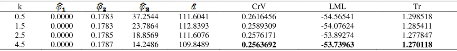
TABLE 2. Criteria for selecting the soybean yield model elaborated with covariates considering the covariance function Matérn with different form parameters.
k CrV LML Tr
0.5 0.0000 0.1783 37.2544 111.6041 0.2616456 -54.56541 1.298518
1.5 0.0000 0.1783 23.7864 112.8393 0.2589309 -54.07624 1.285411
2.5 0.0000 0.1785 18.8569 111.6076 0.2576171 -53.89274 1.277847
4.5 0.0000 0.1787 14.2486 109.8489 0.2563692 -53.73963 1.270118
k: form parameter of the Matérn model; CrV: cross validation; : estimator of the nugget effect; : estimator of contribution; :
estimator of the parameter that defines the range; practical range; LML: maximum value of the logarithm of the likelihood function; Tr:
trace of covariance matrix. The values in bold indicate the best fit for the covariance matrix according to the used criterion.
According to the fitted Gaussian linear spatial model (GSLM), the value associated with the potassium content (K) (Table 3) was the highest and presented a positive sign, indicating that it was the covariate that contributed the most to an increase in the average of the soybean yield (t ha-1). This result corroborates with the
study of Dos Passos et al. (2015), considering that this nutrient is the second most absorbed by the soybean plant, being essential for the growth and development of the
plants (Li et al., 2015). The estimates of the parameters associated to the covariates of phosphorus (P) and manganese (Mn) contents indicated that these covariates contributed little to the estimated soybean yield (Table 3).
The fact that the nugget effect is null indicates that, at small distances, spatial dependence is also small (Vieira & Gonzalez, 2003), meaning that the distances considered among the samples were adequate.
TABLE 3. Estimated parameters for the linear spatial model by the maximum likelihood method considering the covariance function Matérn with form parameter k = 4.5.
4.54 0.06 0.06 0.85 -0.01 0.00 -0.44 0.00 0.18 14.25
(6.8e-1) (5e-2) (6e-2) (3e-1) (1e-3) (1e-3) (1.8e-1) (8e-2) (9e-2) (9.8e-1)
: intercept; parameter estimator associated with to variable i = {Ca, Mg, K, P, Mn, PH}, Ca: calcium content(cmolc dm-3), Mg:
magnesium (cmolc dm-3), K: potassium (mg dm-3), P: phosphorus (mg dm-3), Mn: manganese (mg dm-3), pH: soil pH; : estimator of the
nugget effect; :estimator of contribution ; : estimator of the parameter that defines the range. The values in parentheses correspond to
the standard deviation of each estimated parameter.
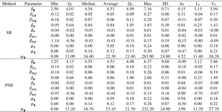
To evaluate the reliability of the parameter estimates, the descriptive statistics of the bootstrap replicates obtained by the BS and BSP methods were calculated and the Efron percentile confidence intervals were determined (Table 4).
From the B = 1000 models adjusted by the BS method, two models (0.2%) were excluded. By the BSP method, only one model (0.1%) was excluded. These exclusions were carried out due to, in these settings; the radius of spatial dependence was greater than the maximum distance between samples (1766 m) in the monitored area. As pointed out by Dalposso et al. (2009), the models that present this behavior should be discarded, considering information that goes beyond the area under study.
For both bootstrap methods, the confidence intervals for the parameters associated with calcium (CA),
magnesium (Mg) and manganese (Mn) contents were zero, indicating that these covariates may not be significant (Table 4).
TABLE 4. Descriptive statistics and Efron percentile 95% confidence intervals of the bootstrap distribution of the model parameters of the spatial dependence structure of soybean yield considering the covariates Ca, Mg, K, P, Mn and pH.
Method Parameter Min Q1 Median Average Q3 Max SD As LL UL
SB
2.50 4.03 4.54 4.53 4.99 7.16 0.71 0.15 3.15 5.94 -0.12 0.02 0.05 0.05 0.09 0.27 0.06 0.31 -0.04 0.17 -0.16 0.02 0.07 0.06 0.11 0.28 0.07 -0.11 -0.07 0.20 -0.05 0.64 0.84 0.84 1.05 1.83 0.30 0.01 0.25 1.43 -0.04 -0.02 -0.01 -0.01 -0.01 0.01 0.01 -0.04 -0.03 -0.00 -0.00 0.00 0.00 0.00 0.01 0.01 0.00 -0.02 -0.00 0.01 -1.14 -0.56 -0.43 -0.43 -0.31 0.15 0.19 -0.15 -0.80 -0.09 0.00 0.00 0.00 0.05 0.10 0.24 0.06 0.90 0.00 0.18 0.00 0.05 0.14 0.12 0.17 0.30 0.07 -0.47 0.00 0.21 0.00 13.00 16.40 22.30 21.40 283.00 24.80 4.52 11.40 26.20
PSB
2.25 4.13 4.55 4.53 4.98 6.37 0.68 -0.09 3.12 5.86 -0.14 0.02 0.06 0.06 0.10 0.23 0.06 -0.18 -0.05 0.17 -0.18 0.02 0.06 0.06 0.10 0.26 0.06 0.01 -0.06 0.19 -0.08 0.66 0.86 0.86 1.06 2.06 0.31 -0.00 0.23 1.49 -0.04 -0.02 -0.01 -0.01 -0.01 0.01 0.01 0.04 -0.03 -0.00 -0.00 0.00 0.00 0.00 0.01 0.01 0.00 -0.04 -0.00 0.01 -0.97 -0.56 -0.44 -0.44 -0.33 0.13 0.18 0.09 -0.79 -0.07 0.00 0.00 0.00 0.05 0.10 0.22 0.06 0.94 0.00 0.18 0.00 0.06 0.14 0.12 0.17 0.28 0.07 -0.50 0.00 0.22 0.00 13.20 16.70 23.10 21.70 232.20 24.90 3.99 11.70 27.70
SB: spatial bootstrap, PSB: parametric spatial bootstrap, : model intercept, : parameter estimate associated with to variable i = {Ca, Mg,
K, P, Mn, PH}, Ca: calcium content(cmolc dm-3), Mg: magnesium (cmolc dm-3), K: potassium (mg dm-3), P: phosphorus (mg dm-3), Mn:
manganese (mg dm-3), pH: soil pH; :nugget effect, : contribution, : range parameter, Min: minimum, Q1: first quartile, Q3: third
quartile, Max: maximum, SD: standard deviation, As: asymmetry coefficient, LL: lower limit of the confidence interval, UL: upper limit of
the confidence interval.
When comparing the standard deviations of the model parameters (Table 3), with the respective standard deviations obtained by the bootstrap (Table 4), except for the standard deviation of the range parameter ( ), the others presented similar values. In the analysis of significance of the GSLM parameters (Table 5) the
hypotheses , and
are not rejected at 5% significance, demonstrating that spatial bootstrap methods are an alternative to test the individual effect of covariates.
Due to the parameters associated with calcium (Ca, cmolc dm-3), magnesium (Mg, cmolc dm-3) and manganese
(Mn, mg dm-3) contents were not significant (Table 5), a
new spatial linear model considering potassium (K, mg dm-3), phosphorus (P, mg dm-3) and soil pH was adjusted,
which presented significant parameters.
TABLE 5. Likelihood ratio test (LR) value and p-value for
hypotheses , in
the linear spatial model.
Null hypothesis LR p-value 1.18 0.2033 0.86 0.2782 7.68 0.0030 * 4.40 0.0211 * 2.76 0.0604 5.66 0.0098 *
LR: likelihood ratio test, p-value: descriptive level of the test at 5% significance.
According to the CrV, LML and Tr criteria, the best fit for the GSLM was provided by the Matérn model with parameter of k form = 4.5 (Table 6).
TABLE 6. Parameters estimated by ML for the linear spatial model considering the covariance function Matérn with form parameter k = 4.5 and the covariates K, P and pH.
3.99 0.84 -0.01 -0.16 0.00 0.19 13.14 (4.9e-1) (3e-1) (1e-3) (1e-1) (1.1e-1) (1.2e-1) (9.3e-1)
ML: maximum likelihood; : intercept; parameter
estimator associated with the variable i = {K, P, PH}, K:
potassium (mg dm-3), P: phosphorus (mg dm-3), pH: soil pH; :
estimator of the nugget effect; :estimator of the
contribution; : estimator of the parameter that defines the range. The values in parentheses correspond to the standard deviation of each estimated parameter.
Comparing the complete model (Table 3) with the model elaborated with the covariates identified as significant (Table 6), the value associated with potassium content (K) remained high and positive. The value near zero of the parameter associated with the phosphorus content indicates that its influence on the average yield is minimal.
decreases the availability of the micronutrients (Sousa et al., 2007), which, consequently, can result in yield losses.
Observing the productivity contour map (Figure 2) elaborated with the parameters of the fitted spatial linear model (Table 6), the majority of the area (84%) presented yield values varying from 3.175 t ha-1 to 3.592 t ha-1.
FIGURE 2. Map of soybean yield generated using kriging with external drift.
Another characteristic observed in the soybean yield map (Figure 2) is the presence of circular regions centered on the sample points. These regions represent the phenomenon known as bull eyes effect that, as explained by Menezes et al. (2016), it occurs when the model has a spatial dependence radius less than the distance between neighboring sample points. Analyzing the distances between the pairs of sample points in the monitored area (Figure 1), only 33 pairs of points (0.68%) had a distance less than the spatial dependence radius (121 m). Thus, for presenting a behavior similar to a pure nugget effect, as highlighted by Margalho et al. (2014), the map was expected to show constant values.
Analyzing the q-q plot chart (Figure 3), traced points are on or near the straight line that passes through
the ordered pairs
( and
( that
and represent, respectively, the quantiles of order 0.25 and 0.75. As Fowlkes (1987) explained, this fact indicates that the theoretical quantis are in agreement with the quantis observed; therefore, it is coherent to assume that the data of soybean yield follow a normal distribution.
FIGURE 3. Quantile-quantile plot of soybean yield (t ha-1).
In particular, the straight line that passes through ordered pairs formed with quantiles of order 0.25 and 0.75.
CONCLUSIONS
The SB and PSB methods allowed to quantify the uncertainties associated to the spatial dependence structure and to evaluate the individual significance of the parameters associated to the average of the spatial linear model, allowing the determination of a model with a smaller number of parameters.
The fact that the linear spatial model formed with the potassium (K, mg dm-3), phosphorus (P, mg dm-3) and
soil pH covariates had a spatial dependence radius close to the minimum distance between points, provided a map characterized by circular regions and a high amount of near-average values.
The use of the uncorrected residuals in the q-q plot elaboration allowed verifying the normality assumption of the soybean yield data, a presupposition that, in many cases, is simply assumed without verification. This finding is extremely important in the analysis since a violation of the normality assumption can invalidate statistical hypothesis tests.
ACKNOWLEDGEMENTS
The authors would like to thank to UTFPR, UNIOESTE, UFPE, FUNDAÇÃO ARAUCÁRIA and CAPES and to the Fondecyt Project 1150325 - Chile for the support provided to carry out this study.
REFERENCES
Aparecido LE, Rolim GS, Richetti J, Souza PS, Johann JA (2016) Köppe, Thornthwaite and Camargo climate classifications for climatic zoning in the State of Paraná, Brazil. Ciência e Agrotecnologia 40(4):405-417. DOI: http://dx.doi.org/10.1590/1413-70542016404003916 Ávila MR, Albrecht LP (2010) Isoflavonas e a qualidade das sementes de soja. Informativo Abrates 20(1):15-29. Borssoi JA, Uribe-Opazo MA, Galea M (2011) Técnicas de diagnóstico de influência local na análise da
produtividade da soja. Engenharia Agrícola 31(2):376-387. DOI:
http://dx.doi.org/10.1590/S0100-69162011000200018
Conab (2016) Soja – Brasil: Série histórica de produtividade. Available: http://www.conab.gov.br. Accessed: Nov 17, 2016.
Cressie N (2015) Statistics for spatial data. New York, John Wiley & Sons. 928p.
Cruz SCS, Sena-Junior DG, Santos DMA, Lunezzo LO, Machado CG (2016) Cultivo de soja sob diferentes densidades de semeadura e arranjos espaciais. Revista de Agricultura Neotropical 3(1):1-6.
Dalposso GH, Uribe-Opazo MA, Borssoi JA, Johann JA, Mercante E (2009) Previsão da produção de trigo
utilizando métodos geoestatísticos. In: Di Leo N, Montico S, Nardón G. Avances en Ingenieria Rural 2007-2009. Rosario, Editorial de la Universidad Nacional de Rosario. p78-86.
De Bastiani F, Cysneiros AHMA, Uribe-Opazo MA, Galea M (2015) Influence diagnostics in elliptical spatial linear models. Test 24(2):322-340. DOI:
http://dx.doi.org/10.1007/s11749-014-0409-z
Diggle PJ, Ribeiro-Jr PJ (2007) Model–based geostatistics. New York, Springer. 232p.
Dos Passos AMA, Rezende PM, Carvalho ER, Ávila FW (2015) Biochar, farmyard manure and poultry litter on chemical attributes of a Distrophic Cambissol and soybean crop. Revista Brasileira de Ciências Agrárias 10(3):382-388. DOI: http://dx.doi.org/10.5039/agraria.v10i3a4546 Efron B (1979) Bootstrap methods: Another look at the jackknife. Annals of Statistics 7(1):1-26
Efron B (1982) The jackknife, the bootstrap and other resampling plans. Philadelphia, SIAM. 93p.
Embrapa (2009) Sistema brasileiro de classificação de solos. Rio de Janeiro, Embrapa.
Fowlkes EB (1987) A folio of distributions: A collection of theoretical quantile quantile plots (78). New York, Marcel Dekker. 560p.
Gallon M, Buzzello GL, Trezzi MM, Diesel F, Silva HL (2016) Ação de herbicidas inibidores da PROTOX sobre o desenvolvimento, acamamento e produtividade da soja. Revista Brasileira de Herbicidas 15(3):232-240. DOI: http://dx.doi.org/10.7824/rbh.v15i3.471
Guedes LPC, Ribeiro-Jr PJ, Uribe-Opazo MA, De Bastiani F (2016) Mapas da produtividade da soja usando
configurações amostrais regulares e otimizadas pela têmpera simulada. Engenharia Agrícola 36(1):114-125. DOI:
http://dx.doi.org/10.1590/1809-4430-Eng.Agric.v36n1p114-125/2016
Gupta SK, Manjaya JG (2016) Assessment of genetic variation at soybean mosaic virus resistance loci in Indian Soybean (Glycine max L. Merill) genotypes using SSR markers. Eletronic Journal of Plant Breeding 7(2):392-400. DOI: http://dx.doi.org/10.5958/0975-928X.2016.00048.X Kang C, Choi S, Yoo SH (2008) A spatial bootstrap method for kriging variance. Journal of the Korean Data Analysis Society 10(3):1247-1254.
Kestring FBF, Guedes LPC, De Bastiani F, Uribe-Opazo, MA (2015) Comparação de mapas temáticos de diferentes grades amostrais para a produtividade da soja. Engenharia Agrícola 35(4):733-743. DOI:
http://dx.doi.org/10.1590/1809-4430-Eng.Agric.v35n4p733-743/2015
Li L, Xu L, Wang X, Pan G, Lu L (2015) De novo characterization of the alligator weed (Alternanthera philoxeroides) transcriptome illuminates gene expression under potassium deprivation. Journal of Genetics 94(1):95-104. DOI: http://dx.doi.org/10.1007/s12041-015-0493-1 Mardia KV, Marshall RJ (1984) Maximum likelihood estimation of models for residual covariance in spatial regression. Biometrika 71(1):135-146. DOI:
http://dx.doi.org/10.2307/2336405
Margalho L, Menezes R, Souza I (2014) Assessing interpolation error for space-time monitoring data. Stochastic Environmental Research and Risk Assessment 28(1):1307-1321. DOI: http://dx.doi.org/10.1007/s00477-013-0826-7
Matérn B (1986) Spatial variation. Berlin, Springer-Verlag, 2 ed. 151p.
Menezes MD, Silva SHG, Mello CR, Owens PR, Curi, N (2016) Spatial prediction of soil properties in two contrasting physiographic regions in Brazil. Scientia Agricola 73(3):274-285. DOI:
http://dx.doi.org/10.1590/0103-9016-2015-0071
Olea RA, Pardo-Igúzquiza E (2011) Generalized bootstrap method for assessment of uncertainty in semivariogram inference. Mathematical Geosciences 43(2):203-228. DOI: http://dx.doi.org/10.1007/s11004-010-9269-6.
Pardo-Igúzquiza E, Olea RA (2012) VARBOOT: A spatial bootstrap program for semivariogram uncertainty
assessment. Computers & Geosciences 41(1):188-198. DOI: http://dx.doi.org/10.1016/j.cageo.2011.09.002. Pimentel Gomes, F (1985) Curso de estatística experimental. São Paulo, Nobel. 467p.
R Core Team (2017) R: A language and environment for statistical computing. R foundation for statistical computing. Vienna.
Rao CR (1973) Linear statistical inference and its applications. New York, John Wiley e Sons. 656p. Schelin L, Sjöstedt-De Luna S (2010) Kriging prediction intervals based on semiparametric bootstrap, Mathematical Geosciences 42(1):985-1000. DOI:
http://dx.doi.org/10.1007/s11004-010-9302-9 Sjöstedt-De Luna S, Young (2003) The bootstrap and kriging prediction intervals. Scandinavian Journal of Statistics 30(1):175-192.
Solow A (1985) Bootstrapping correlated data. Mathematical Geology 17(7):769-775. DOI: http://dx.doi.org/10.1007/BF01031616
Sousa DMG, Miranda LN, Oliveira AS (2007) Acidez do solo e sua correção. In: Novais RF, Alvarez VH, Barros NF, Fontes RL, Cantarutti RB, Neves JCL. Fertilidade do solo. SBCS, p205-274.
Tang L, Schucany W, Woodward W, Gunst R (2006) A parametric spatial bootstrap. Technical Report SMU-TR-337. Dallas, Southern Methodist University.
Tomé Jr JB (1997) Manual para interpretação de análise de solo. Guaíba, Agropecuária. 247p.
Uribe-Opazo MA, Borssoi JA, Galea, M (2012) Influence diagnostics in gaussian spatial linear models. Journal of Applied Statistics 3(39):615-630. DOI: