Palavras chave:
Amostragem proporcional Amostragem com igual frequência Distribuição diamétrica Acurácia em equações de volume Avaliação de resíduos
Histórico:
Recebido 25/03/2016 Aceito 14/07/2016
Keywords:
Proportional sampling Even-frequency sampling Diameter distribution Accuracy of volume equations Examination of residuals
1 Federal University of Paraná - Curitiba, Paraná, Brasil
2 AFM Forest company - Charlotte, North Caroline, Estados Unidos Correspondência:
DOI:
10.1590/01047760201622032155
Hassan Camil David1, Rodrigo Otávio Veiga Miranda1, John Welker2, Luan Demarco Fiorentin1, Ângelo Augusto Ebling1, Pedro Henrique Belavenutti Martins da Silva1
STRATEGIES FOR STEM MEASUREMENT SAMPLING: A STATISTICAL APPROACH OF MODELLING INDIVIDUAL TREE VOLUME
ABSTRACT: The aim of this paper was to evaluate different criteria for stem measurement sampling and to identify the criterion with best performance for developing individual tree volume equations. Data were collected in eucalyptus stands 58 to 65 months old. Schumacher-Hall model was applied using five sampling criteria with nine variations (45 in total): 1) number of trees per diameter class, being (a) fixed number, (b) proportional to the diameter class of the sample, or (c) proportional to the standard deviation of the sample; and 2) the width of the diameter class, which ranged from 1.0 up to 5.0 cm. We used the equations generated from each of the five sampling criteria to estimate stem volume of trees reserved for validation. This allowed us to obtain standard errors of estimates from this data-set. In addition, residuals of volume estimates were examined by means of statistical tests of bias, autocorrelation and heteroscedasticity. Better performances of volume equations occurred when smaller diameter class widths were used, i.e., when the sample size increased. There was no clear trend in increasing/decreasing residual autocorrelation and/or heteroscedasticity. Both methods of sampling proportional to the frequency of diameter class had the best performances, inclusive using only 36 trees. The ones where choice of trees was proportional to the standard deviation had the worst. In conclusion, the selection proportional to the frequency of the diameter class, under the condition that at least two trees per class are sampled, provides models statistically better than all the other criteria.
ESTRATÉGIAS DE AMOSTRAGEM DE FUSTES PARA MEDIÇÃO: UMA ABORDAGEM ESTATÍSTICA DA MODELAGEM DO VOLUME DE ÁRVORE INDIVIDUAL
INTRODUCTION
Linear and non-linear models have an extensive usage in forest mensuration, in large part because they provide reliable estimates of independent variables. Besides, the availability of software for obtaining coeffi cients, and their ease of application are good reason for using regression models.
The formulation of models corresponds to an important step in independent variable estimation, since it is desirable for the sample estimators to have predictions and confi dence intervals that are unbiased and accurate. For this to occur, some assumptions of the classical linear regression model must be satisfi ed to obtain unbiased, consistent and effi cient estimators, also known as Best Linear Unbiased Estimator (BLUE). The properties of Ordinary Least Squares (OLS) estimators require that the residues ( ) possess average equal to zero, be non-autocorrelated and present fi xed variance, i.e., homoscedastic and independence (GUJARATI; PORTER, 2009; LISTA, 2014).
Due to the fact that accurate wood volume estimation is one of the most important variables of interest in a forest inventory, it is highly desirable that volume equations present BLUE estimators. Volume regression models require a set of tree (felled or not) measurements sampled from the forest inventory population of interest. These measurements must come from a well-representative sample. Thus, the selection of trees for scaling is an important step in modelling individual tree volume, besides being a costly one.
In Brazilian forest inventories, usually the selection of trees for scaling is done throughout the population being inventoried and traditionally the number of trees to be scaled is fi xed by diameter class (CAMPOS; LEITE, 2013), ranging from 4 to 6 trees per class (SOARES et al., 2011). Empirically there are suggestions of up to 10 trees if the width of the diameter class is 5 cm (MUGASHA et al., 2016). In fact, there is a lack of evaluation concerning number of trees to be sampled and how this affects volume model capabilities. Perhaps such recommendations are conclusions of empirical methods and stabilization of coeffi cient of variation.
However, this sampling criterion of equal numbers of trees selected by diameter class corresponds probabilistically to a rectangular distribution. Thereby, we observe that there is not a concordance between such criterion of choosing trees and the Gaussian distribution observed in even-aged stands (BINOTI et al., 2015).
The traditional approach to sampling presents the interesting advantage of including the variability of stem
form across all diameter classes. Operationally, one of the disadvantages found on the traditional sampling is the requirement of fi nding and measuring trees that are less frequent, i.e, trees in extreme classes (PICARD et al., 2012).
On the other hand, proportional-to-frequency sampling may require less time and labor cost because most of the measured trees occur more frequently. Assuming a normal diameter distribution, this sampling favors trees sampled closer to the average, since it disfavors trees in extreme classes. In addition, this sampling contemplates those classes most frequently found in the forest population. Thus, it forces the estimators to converge in values closer to the populational estimators, due to the weighting of the tree frequency by diameter class (PICARD et al., 2012).
We initiated this study assuming the following hypothesis: the criteria for choosing sampled trees for stem volume affects the accuracy of individual tree volume equations. The aim of this paper was to select a criterion for stem measurement sampling which has best performance for modelling individual tree volume.
MATERIAL AND METHODS Study area and data collection
The database came from a forest inventory carried out in a hybrid eucalyptus forest(Eucalyptus grandis W. Hill ex Maiden x Eucalyptus urophylla S. T. Blake), 58 to 65 months old. The planted area corresponds to 558.7 ha, located in north of the state of Bahia, Brazil. The forest present a mean density of 1,111 plants.ha-1.
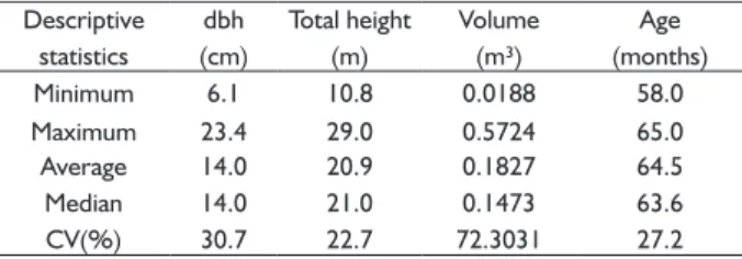
We used data from 57 permanent plots of 471.4 m² each. The variables scaled in the inventory were diameter at breast height, total height and stem volume. The main descriptive statistics of these variables are presented in Table 1.
TABLE 1 Descriptive statistics of the data set used in analysis. Descriptive
statistics
dbh
(cm)
Total height
(m)
Volume
(m³)
Age
(months)
Minimum 6.1 10.8 0.0188 58.0
Maximum 23.4 29.0 0.5724 65.0
Average 14.0 20.9 0.1827 64.5 Median 14.0 21.0 0.1473 63.6
CV(%) 30.7 22.7 72.3031 27.2
dbh: diameter at breast height; CV: coeffi cient of variation.
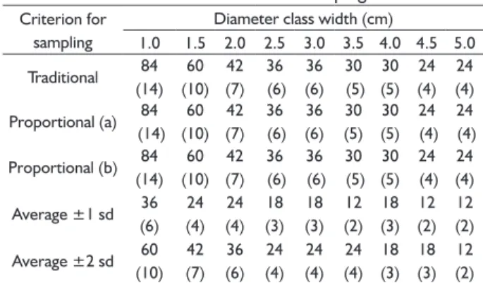
Criteria for tree measurement sampling
The proposal of this work consisted of statistically analyzing the effect of different sampling criteria for tree measurement on modelling individual tree volume. Equations generated for each criterion were used to estimate stem volume of trees reserved to validate the equations, allowing us to reach conclusions about the goodness of fit, biases, autocorrelation and heteroscedasticity of the residuals.
We sampled six trees per diameter class. Furthermore, within a class trees are chosen to represent the lower, mid and upper limit of each diameter class. In this paper, we refer to this criterion of selection as “traditional sampling”.
Basing on our initial hypothesis, we formulated alternative sampling procedures with the objective of developing a better sampling criteria for individual tree volume modelling. Thus, the criterion named as “traditional sampling” was compared with the following alternative criteria:
“Proportional sampling (a)”: the number of trees sampled per diameter class depends on the diameter distribution of the forest population. Thereby, the ratio of the number of trees per class and the total number was used as the weighting factor for each class;
“Proportional sampling (b)”: similar to the previous criterion, however we added the condition that ensures at least 2 trees are sampled per class;
“Average ±1 deviation sampling”: it consists of selecting only the trees inside the interval of ±1 standard deviation around the average diameter of the sample. Therefore, the minimum and maximum diameter classes reach the average minus and plus one standard deviation, respectively;
“Average ±2 deviations sampling”: similar to the criterion previously described, but using two rather than one standard deviation.
These five criteria (traditional and the alternatives) were repeated nine times, since we tested arbitrarily nine diameter class widths that ranged from 1.0 up to 5.0 cm, resulting in 45 strategies for stem measurement sampling. Table 2 presents the number of trees and diameter classes in each strategy. Each diameter class width implies in varying the number of felled-tree samples.
The “traditional sampling” criterion always sampled six trees per diameter class, since it is a common practice used by many companies. This ceiling
number was also used to establish the number of trees per class in the criteria with standard deviation, in order to permit a better comparison with the “traditional sampling” criterion.
TABLE 2 Number of trees and of diameter classes (in brackets) of criteria for stem measurement sampling.
Criterion for sampling
Diameter class width (cm)
1.0 1.5 2.0 2.5 3.0 3.5 4.0 4.5 5.0 Traditional 84 (14) 60 (10) 42 (7) 36 (6) 36 (6) 30 (5) 30 (5) 24 (4) 24 (4) Proportional (a) 84
(14) 60 (10) 42 (7) 36 (6) 36 (6) 30 (5) 30 (5) 24 (4) 24 (4)
Proportional (b) 84 (14) 60 (10) 42 (7) 36 (6) 36 (6) 30 (5) 30 (5) 24 (4) 24 (4)
Average ±1 sd 36
(6) 24 (4) 24 (4) 18 (3) 18 (3) 12 (2) 18 (3) 12 (2) 12 (2)
Average ±2 sd 60
(10) 42 (7) 36 (6) 24 (4) 24 (4) 24 (4) 18 (3) 18 (3) 12 (2) sd: standard deviation
In the criteria with standard deviation, the number of classes depended on the value of such statistical estimator. Two standard deviations around the average will encompass more classes than one standard deviation, mainly when the diameter class width is a small value.
Therefore, both sampling based on standard deviation as the “traditional sampling” are equivalent in number of trees per class but different in total number of trees sampled. Similarly, the traditional and proportional sampling criteria are equivalent in total number of trees but different in number of trees per class, as shown in Table 2.
For example, Figure 1 illustrates the sampling frequency by diameter class considering a diameter class width of 1.0 cm. Bars indicate the relative frequency of trees established on the criterion and the lines indicate the real relative frequency of trees observed in the forest.
There is a criterion for sampling usually adopted in forest inventories, but not employed by us, which consists of measuring more trees in classes with high diameter variations. We opted not to test such method because the variation by diameter class is higher in classes belonging to small trees, whose value of logs is much low comparing to the bigger ones. Therefore, it is more important to sample larger trees for enhancing their estimates.
Volume model and comparison of coefficients After creating data sets for each of the five different sampling criteria and their nine variations, we fitted the model of Schumacher-Hall using a database related to each sampling strategy, thus obtaining 45 equations of stem volume. We took the logarithm of the original model (VIBRANS et al., 2015), resulting in the
2 2
i i
i
(D d )
v L
80000
+
linear model [2], where: ln = natural logarithm; v=stem volume in m³; dbh=diameter at breast height in cm; h=total height in m; β0 to β2 = parameters of the model to be estimated; εi= random error.
0 1 2 i
ln(v)= b + b ln(dbh)+ b ln(h)+ e [2]
We estimated the parameters using the Ordinary Least Squares (OLS) method. Coeffi cients of equations obtained with the “traditional sampling” had their confi dence intervals estimated by means of Student t-test at 95% probability level. They were plotted in graphs along with the coeffi cients of all criteria. This comparison helps identify discrepancies between equations belonging to each sampling criterion.
Validation of the methodology
In order to validate the equations, we created a validation database with 28 felled and scaled trees that were not used in the equation development. The number of trees per diameter class in this validation database were randomly selected and had the same diameter distribution frequency as that in the forest inventory population, i.e., the frequency of trees per class was proportionally equivalent to the diameter distribution.
The comparisons and statistics to evaluate residuals and goodness of fi t (equations 3 to 6) were all calculated and based on these validation data.
Evaluation of estimated residuals and goodness
of fi t
We evaluated the estimated residuals by means of statistics that detect problems of bias, autocorrelation and heteroscedasticity. We applied the Durbin and Watson (1951) test [3] to detect residual autocorrelation. The calculation is given as follows (DAVID et al., 2015), where: = Residuals of ith observation; = Pearson
correlation coeffi cient; n = number of observations.i
ˆ
e
r
ˆ
n 2
i i 1 i 2
n 2 i i 1 (ˆ ˆ ) DW
ˆ
-=
=
e - e =
e
å
å
[3]Knowing that ranges from -1 to +1, DW test may assume values between 0 and 4. The test takes into account critical values that divide this interval in zones (0 to 4), being: one positive autocorrelation and one negative autocorrelation zone, one non-autocorrelation zone and two indecision zones. The conclusion about the autocorrelation depends on the zone in which the DW value fi ts.
The hypotheses to be tested are: H0: No positive autocorrelation; H0*: No negative autocorrelation; Ha: Residual autocorrelation.
To evaluate the heteroscedasticity, i.e., if the residual variance is nonconstant, we applied the White
or DW=2(1- rˆ)i = 1, 2,..., n
A.Traditional sampling
B.Proportional sampling
C. Proportional sampling
D. Average ±2 deviations sampling
E. Average ±2 deviations sampling
(1980) statistic [4]. This test consists of fi tting an auxiliary model using as dependent variable the squared residuals from the original regression, and the original X variables, combined or not, as explanatory variables (DAVID et al., 2015). Where: i
^
e = Residuals of ith observations; αi= artifi cial coeffi cients; x = dependent variable; v = artifi cial residual; k = number of variables, n = number of observations.
Knowing that the “proportional sampling (C)” criterion was defi ned to have at least two trees per class, we could expect that all the coeffi cients were inside the confi dence intervals, due to its closer similarity to the “traditional sampling” criterion. However, such condition was not enough to obtain statistic equality of all the coeffi cients.
Concerning the “Average ±1 deviation sampling” criterion, almost all the diameter class widths had at least one coeffi cient that exceeded the confi dence intervals from the coeffi cients of the “traditional sampling”. The exception occurred only for the class width of 4.0 cm, in which all the coeffi cients were inside the limits.
In the of 4.0 and 5.0 cm diameter class widths the number of trees were equal for both of the standard deviation sampling criteria (Table 2). Therefore, the same trees were selected for modelling and the coeffi cients are identical. Considering the other seven diameter class widths, the “Average ±2 deviations sampling” criterion presented coeffi cients statistically within the confi dence limits of those obtained in the “traditional sampling”.
k k
in j 1 k j s ij ik
ˆ
= =x x
v
e = a +
å å
a
+
i = 1,..., n; j = 1,…, k; s = 1,…, k.(k+1).2-1
[4]
Homoscedasticity is detected when nR2 < , otherwise the residuals are heteroscedastic; where: n = number of observations; R² = coeffi cient of determination; χ² = chi-squared; DF = number of parameters of the artifi cial model (without intercept).
We also evaluated the accuracy of the individual tree volume equations using the standard error of the estimate (SEE%) [5]. Moreover, we used residual ( %) [6] graphs to detect presence of bias, where: yi and = observed and estimated variables of the ithobservation; = average of observed variable; n = number of observations; p = number of coeffi cients excluding the intercept.
ˆ
e
2 DF
c
n 2 i i 1(y y )ˆ 100
SEE(%) .
n p y
=
-=
-å [5]
i ˆi (y y ) ˆ(%) .100
yi
-e = [6]
RESULTS AND DISCUSSION
Coeffi cients of individual tree volume equations
In order to answer the hypothesis of this study, we compared the sampling criteria with the traditional method. At fi rst, we plotted the estimated coeffi cients
β
0,β
1 andβ
2 (Figure 2), as well as the confi dence intervals obtained with the “traditional sampling”.Except in a few cases, a high number of model coeffi cients from the alternative sampling strategies occurred within the “traditional sampling” confi dence intervals across all diameter class widths.This result shows the similarity of tree volume equation estimators regardless of the sampling criterion.
The similarity of the results is highest with the “proportional sampling (B)” and “proportional sampling (C)” criteria. Across all nine class widths, only the class width equal to 4.5 cm had coeffi cients exceeding the limits.
A.
B.
D.
FIGURE 2 Coeffi cients from the volume equations fi tted to criteria for stem measurement sampling. Graylines: confi dence intervals of coeffi cients of the “traditional sampling”. The numbers inside the graphs represent the diameter class width.
A. B. C.
Examination of the residuals
Figure 3 presents scatterplots of residuals in relation to diameters at breast height. Each row of graphs is associated with a particular diameter class width, and each column is associated with a particular sampling criterion.
Even though the criteria differ in the total number of measured trees and in sampling criterion, these differences did not result in biased estimations in the majority of cases. The worst situations were seen in the diameter class width of 5.0 cm, in which the criteria using
FIGURE 3 Residuals from the estimated volumes. X axis: Dbh (cm); Y axis: (Residual error in %).
standard deviation presented wider dispersions and smooth positive correlations (Figure 3).
The “traditional sampling” and “proportional sampling (a) and (b)” criteria presented equations with the best unbiased estimators, even for the diameter class width of 5.0 cm (Figure 3).
The “Average ±1 deviation sampling” criterion had performance worse than the one with two standard deviations. Moreover, except for the diameter class width of 5.0 cm, the “Average ±2 deviations sampling” criterion presented performance similar to the “proportional sampling” criteria.
Basing on Figure 3, the number of sampled trees had less effect on the residual dispersion than the sampling criterion itself. For example, the samplings with deviations and using class width of 5 cm contemplate 12 sampled trees. This sample number also was used in other class widths, where the residual dispersion had better behavior (Table 2).
In fact, if we analyze the equal sample numbers presented (Table 2) and compare them with their residual graphs (Figure 3), some situations like this occur in other class widths too.
Regarding to the heteroscedasticity and autocorrelation of the residuals, Table 3 presents the results of the Durbin-Watson and White tests for the five criteria for sampling in each class width.
As a complementary analysis, heteroscedasticity was also examined by means of scatterplots presented in Figure 3. This is possible because the bias of estimates is an indication of this problem (GUJARATI; PORTER, 2009).
The autocorrelation of the residuals, in turn, may be detected by the scatterplots showed in Figure 4. Each row of graphs is associated with a particular diameter class width, and each column is associated with a particular sampling criterion.
The diameter class width of 1.0 cm had the best performance to avoid heteroscedasticity and autocorrelation of the residuals (Table 3). This was the only diameter class width free of this problem regardless of the criterion for sampling. On the other hand, the 5.0 cm diameter class width was the worst alternative for avoidance of such problems.
However, heteroscedasticity and autocorrelation of the residuals were present in all criteria, at least in two diameter class widths; therefore, we must be aware that no criterion is absolutely free of this problem. The “Average ±1 deviation sampling” was the most prone to such problems and this corroborates the results already presented in Table 3.
The stronger autocorrelations of residuals were identified in cases with biased estimations such as the ones presented in the diameter class width of 5.0 cm, as well as in the “Average ±1 deviation sampling” criterion (Figure 4).
Gujarati and Porter (2009) elucidate that the consequences of the presence of heteroscedasticity and autocorrelation, although the OLS estimators are linear, unbiased and normally distributed, under both problems, are no longer minimum variance among all linear unbiased estimators. Therefore, the usual Student’s t-test, F-test and may not be valid.
TABLE 3 Tests of autocorrelation and heteroscedasticity of the residuals for the stem measurement sampling criteria.
Class width Test Traditional (A) Proportional (B) Criterion for samplingProportional (C) Average ±1 sd (D) Average ±2 sd (E) 1.0 DW No autocorrelation No autocorrelation No autocorrelation No autocorrelation No autocorrelation W Homoscedastic Homoscedastic Homoscedastic Homoscedastic Homoscedastic 1.5 DW No autocorrelation No autocorrelation No autocorrelation No autocorrelation No autocorrelation
W Heteroscedastic Homoscedastic Homoscedastic Homoscedastic Heteroscedastic 2.0 DW No autocorrelation Indecision zone No autocorrelation Pos. auto-correlation Indecision zone W Homoscedastic Homoscedastic Homoscedastic Heteroscedastic Homoscedastic 2.5 DW Indecision zone No autocorrelation No autocorrelation Pos. auto-correlation Indecision zone W Homoscedastic Homoscedastic Homoscedastic Homoscedastic Homoscedastic 3.0 DW No autocorrelation No autocorrelation No autocorrelation Indecision zone No autocorrelation
W Heteroscedastic Homoscedastic Homoscedastic Heteroscedastic Homoscedastic 3.5 DW No autocorrelation No autocorrelation No autocorrelation Pos. auto-correlation Indecision zone W Homoscedastic Heteroscedastic Homoscedastic Heteroscedastic Heteroscedastic
4.0 DW No autocorrelation No autocorrelation Pos. auto-correlation No autocorrelation No autocorrelation
W Heteroscedastic Homoscedastic Heteroscedastic Homoscedastic Homoscedastic
4.5 DW Pos. auto-correlation No autocorrelation No autocorrelation No autocorrelation Indecision zone
W Heteroscedastic Homoscedastic Homoscedastic Homoscedastic Heteroscedastic 5.0 DW Indecision zone Pos. auto-correlation Pos. auto-correlation Pos. auto-correlation Pos. auto-correlation
W Homoscedastic Heteroscedastic Heteroscedastic Heteroscedastic Heteroscedastic
FIGURE 4 Current residuals related to lagged residuals of volume equations. X axis: ui; Y axis: ui-1.
For fixing this problem, Gujarati and Porter (2009) explain that the error variance of the model may have its variables transformed using the Generalized Least Square method. The transformation of the variables can be done as follows [7] and [8]:
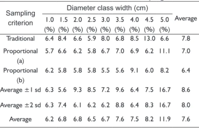
superiorities in relation to the other sampling strategies, in general the “Average ±1 deviation sampling” had the worst performance, followed by the “Average ±2 deviations sampling”.
Likewise, if we compare the class widths, the ones lower than 3.5 cm had the smaller errors. Even though most of the standard errors of the estimate ranged around 6% to 9%, we obtained values exceeding 10%, reaching up to 16.7%, as seen in diameter class widths of 4.5 and 5.0 cm (Table 4).
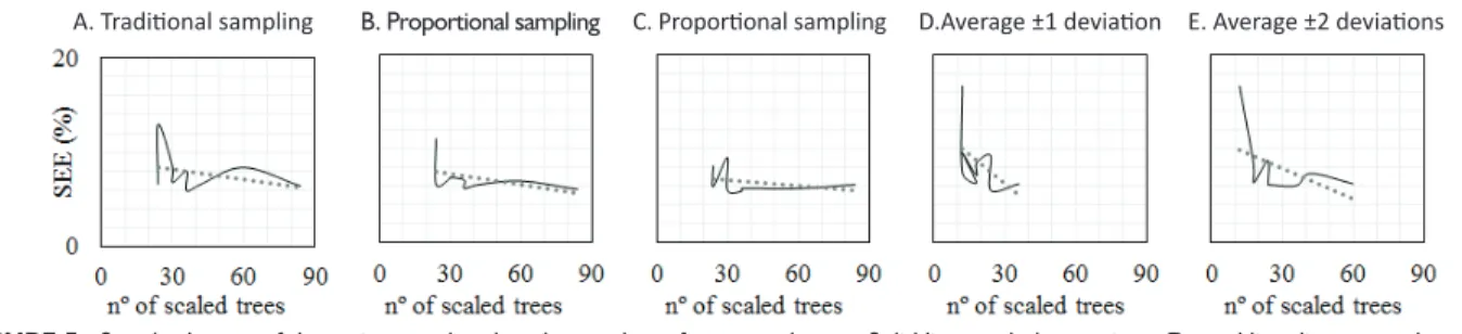
There was a trend in reducing the standard error to the extent that increases the number of measured trees, which is inversely proportional to the size of the class width (Table 2).
Such relation may be weaker or stronger depending on the criterion for sampling. Indeed, the number of trees affected the performance of the volume model, but it was mainly observed when few trees were sampled. More precisely, the larger variations of SEE(%) occurred in those class widths encompassing less than 36 trees (Figure 5), remembering that the minimum was 12 trees for the criteria with standard deviation and 24 trees for the others. Silva et al. (2007) found similar results, but for diameter-height relationship in eucalyptus stands. These authors concluded that the model has no significant improvement in accuracy when the sample size is larger than 27 trees.
We detected stronger correlations between SEE(%) and number of measured trees for the criteria involving standard deviation. Such behavior seems to be caused by its low total number of trees adopted in the regression, mainly in the sampling with one standard deviation.
Due to these two samplings also have six trees per class (such as the “traditional sampling”), the results indicate the serious problem caused by neglecting extreme diameter classes, since these sampling strategies contemplate only one or two standard deviation around the average.
In respect to the proportional sampling (a) and (b), its weaker relation between the SEE (%) and number of measured trees may be associated to the weighting by frequency of diameter classes. In both cases, the errors become stable from 36 measured trees, however, such trend was not so clear in the other criteria. Therefore, the results reveal to be more interesting to fit the volume model with proportional sampling, with no requirement of increasing the number of measured trees.
Leal et al. (2015) also obtained a trivial effect of the number of sampled trees on the accuracy of volume models, however, they used a minimum number of 48 trees when they evaluated proportional samplings. 0
i i i
0 1
i i i i
x
y x
b . b . e
= + +
s s s s [7]
Biased estimators bi become BLUE, in which are represented by in Model [7.2]:
i
* * * * * *
i 0 0 1 i i
y =b x +b x + e [8]
Accuracy of individual tree volume equations
The last analysis concerns the behavior of the standard error of the estimate (SEE), whose calculation was based on the stem volume estimates from the trees of the validation database. The coefficients of the volume equations are those presented in Figure 2. The standard errors of the estimate for all sampling criteria and diameter class widths are showed in Table 4.
TABLE 4 Standard errors of the estimate of the regression models to estimate stem volume using different criteria for stem measurement sampling.
Sampling criterion
Diameter class width (cm)
Average 1.0 (%) 1.5 (%) 2.0 (%) 2.5 (%) 3.0 (%) 3.5 (%) 4.0 (%) 4.5 (%) 5.0 (%)
Traditional 6.4 8.4 6.6 5.9 8.0 6.8 8.5 13.0 6.6 7.8 Proportional
(a)
5.7 6.6 6.2 5.8 6.7 7.0 6.9 6.2 11.1 7.0
Proportional
(b)
6.2 5.8 5.8 5.8 5.5 5.6 9.1 6.0 8.2 6.4
Average ±1 sd 6.3 5.6 9.3 8.5 7.2 9.6 6.4 7.5 16.7 8.6 Average ±2 sd 6.3 7.4 6.1 6.2 6.2 8.8 6.4 8.3 16.7 8.0 Average 6.2 6.8 6.8 6.5 6.7 7.6 7.5 8.2 11.9 7.6
sd: standard deviation
Comparing the errors among the criteria, in general, the “proportional sampling (a) and (b)” provide better model performance, i.e., the smaller error averages (Table 4). The “traditional sampling” was better than the “proportional sampling (a)” for diameter class widths of 3.5 and 5.0 cm, but with respect to “proportional sampling (b)”, the better performance was seen only in the class width of 4.0 cm. Therefore, the condition that ensures at least two measured trees per diameter class, adopted in “proportion sampling (b)”, was a way to enhance the “proportion sampling (a)”.
Main highlights of the tree sampling strategies
There are few researches dealing with strategies for tree measurement sampling. Some cautions must be taken when volume equations are applied, since the residuals may have problems that lead to misleading conclusions about statistical tests.
Regression models presenting problems of residual heteroscedasticity and autocorrelation generate similar consequences on estimates. Estimators of the volume model with overestimated variance is one of the problems. In practice, confi dence interval of the volume is a desirable statistic, however, it is misleading in presence of residual heteroscedasticity and autocorrelation.
Comparing all the criteria presented here, traditional sampling possesses the disadvantage of requiring the scaling of many less frequent trees, making the sampling procedure slower and more expensive operationally. Furthermore, when the demand of sample trees is high, cutting down many larger trees is may not be acceptable by companies, mainly due to its high added value of these trees.
This problem can be mitigated using the sampling proportional to the tree frequency of diameter class. In fact, both alternative sampling procedures seem to make this step (log scaling) of the forest inventory relatively cheaper and faster than when the traditional sampling is used.
However, these are not the only advantages, since the accuracy of the volume model also was pointed out as a positive contribution given by the proportional samplings. Leal et al. (2015) also obtained better performances in stem volume equations with use of sampling proportional to the diameter distribution. They obtained very close accuracies in equations using what we named “traditional sampling” and “proportional sampling (a)”.
In our case, the performance obtained in the “Proportional sampling (b)” was even better than the “Proportional sampling (a)”, in which both are more accurate than the “traditional sampling” when class
widths lower than 3.5 cm are used. Unfortunately Leal et al. (2015) did not present variations of class widths, which prevents us to make possible comparisons.
Even though the proportional samplings do not favor an equal coverage in all diameter class, they do not provoke biases on the volume estimates. Furthermore, most estimators of the volume equations were statistically equal to those obtained in the traditional sampling.
Proportional samplings comply with random sampling cited by Picard et al. (2012). These authors showed the limitation of this procedure for reducing the number of sampled trees, in relation to another optimized sampling, of which needs less trees to obtain a same modeling precision. However, we showed that proportional-to-the-frequency sampling was enough to achieve good accuracy with small sample size.
Finally, sampling with use of standard deviation in the most cases presented accuracy and behavior of the residuals worse than the other sampling strategies. Therefore, this type of sampling strategy is not recommended, mainly in class widths larger than 4.0 cm. Evidently, these statements are done for young trees and the researches are needed to assess older stands, since age affects strongly tree volume relationship (RUCHA et al., 2010).
CONCLUSIONS
Some important considerations should be taken into account to obtain accurate individual tree volume equations in eucalyptus forests. Tree measurement sampling with proportion to diameter distribution, i.e., proportional to the number of trees per diameter class, is more advantageous than the sampling with same number of trees per diameter class.
The measurement of at least 36 trees is enough to obtain good accuracy in stem volume estimations. In situations in which it is not possible to scale 36 trees, proportional sampling also can be used, but with condition of measuring at least 2 trees per diameter class.
A. Traditi onal sampling B. Proportional sampling C. Proporti onal sampling D.Average ±1 deviati on E. Average ±2 deviati ons
REFERENCES
BINOTI, D. H. B.; BINOTI, M. L. M. S.; LEITE, H. G. Modelagem da distribuição diamétrica de povoamentos equiâneos de eucalipto utilizando a função logística generalizada. Revista Árvore, v. 39, n. 4, p. 707-711, 2015.
CAMPOS, J. C. C., LEITE, H. G. Mensuração florestal:
Perguntas e respostas. 4ª edição, Viçosa, Editora UFV, 2013, 605p.
DAVID, H. C.; PÉLLICO NETTO, S.; MIRANDA, R. O. V.; EBLING, A. A.; ARAUJO, E. J. G. A. Behavior of form factor models for pine boles using diameters at relative heights. AJBAS, v. 9, n. 2, p. 204-215, 2015.
DURBIN, J.; WATSON, G. S. Testing for Serial Correlation in Least-Squares Regression. Biometrika, v. 38, n. 1, p. 159-171, 1951.
GUJARATI, D. N.; PORTER, D.C. Basic Econometrics. 5. ed. Boston: McGraw-Hill, 2009. 922p.
LEAL, F. A.; CABACINHA, C. D.; CASTRO, R. V. O.; MATRICARDI, E. A. T. Amostragem de árvores de
Eucalyptus na cubagem rigorosa para estimativa de modelos volumétricos. Revista Brasileira de Biometria, v. 33, n.1, p. 91-103, 2015.
LISTA, L. The bias of the unbiased estimator: A study of the iterative application of the BLUE method. Nuclear Instruments and Methods in Physics Research A, v. 764, p. 82-93, 2014.
MUGASHA, W. A.; MWAKALUKWA, E. E.; LUOGA, E.; MALIMBWI, R. E.; ZAHABU, E. et al. Allometric Models for Estimating Tree Volume and Aboveground Biomass in Lowland Forests of Tanzania. International Journal of Forestry Research, v. 2016, p. 1-13, 2016.
PICARD N.; SAINT-ANDRÉ L.; HENRY M. Manual for building
tree volume and biomass allometric equations: from field measurement to prediction. Food and Agricultural Organization of the United Nations, Rome, and Centre de Coopération Internationale en Recherche Agronomique pour le Développement, Montpellier, 2012, 215 p.
RUCHA, A.; SANTOS, A.; CAMPOS, J.; ANJOS, O.; TAVARES, M. Two methods for tree volume estimation of Acacia melanoxylon in Portugal. Revista Floresta, v. 41, n. 1, p.169-178, 2010.
SILVA, G. F.; XAVIER, A. C.; RODRIGUES, F. L.; PETERNELLI, L. A. Análise da influência de diferentes tamanhos e composições de amostras no ajuste de uma relação hipsométrica para Eucalyptus grandis. Revista Árvore, v. 31, n. 4, p. 685-694, 2007.
SOARES, C. P. B.; NETO, F. P.; SOUZA, A. L. Dendrometria
e inventário florestal. Editora UFV, 2ª ed., 2011, 272 p.
VIBRANS, A. C.; MOSER, P.; OLIVEIRA, L. Z.; MAÇANEIRO, J. P. Generic and specific stem volume models for three subtropical forest types in southern Brazil. Annals of Forest Science, v. 72, n. 6, p. 865-874, 2015.