Job matching, unexpected obligations and retiment decisions

(1)

JOB MATCHING, UNEXPECTED OBLIGATIONS

AND RETIREMENT DECISIONS

Mário Centeno Banco de Portugal and Universidade Técnica de Lisboa

Márcio Corrêa Universidade Técnica de Lisboa

Abstract

Our objective is to investigate the effects of unexpected changes in the worker’s obligations on the decision to retire. We considered, throughout this paper, that the firm does not know the level of the worker’s obligations, and is unable to determine the right moment for the worker to retire. We found that the wage rate decreases when the worker obtains the right to retire and that it is necessary that the retirement benefits be greater than the unemployment insurance in order to have flows of workers from unemployment to retirement, while it is not necessary that this be greater than the wage rate to realize flows of workers from employment to retirement. We also verified that the more difficult it is to obtain the right to retire, the higher will be the job creation flow.

Resumo

Nosso objetivo neste artigo é o de estudar, em um mercado de trabalho caracterizado por fricções, os efeitos de variações inesperadas nas obrigações dos trabalhadores sobre sua decisão de aposentadoria. Consideramos, ao longo deste artigo, que as firmas desconhecem o nível das obrigações dos trabalhadores, não sendo capazes de determinar o momento exato que estes exercem seu direito de aposentadoria.

Veremos, como resultados do modelo, que o salário dos trabalhadores diminui quando estes obtêm o direito de aposentadoria e que é necessário que o benefício de aposentadoria seja maior que o seguro de desemprego, para que existam fluxos de trabalhadores do desemprego para a aposentadoria. Por sua vez, não é necessário que o salário do trabalhador seja maior que o benefício de aposentadoria para que existam fluxos de trabalhadores do emprego para a aposentadoria. Veremos, por fim, que quanto mais difícil for a obtenção do direito de aposentadoria, maior será o fluxo de criação de novos postos de trabalho.

Palavras-Chave: Criação e Destruição de Empregos, Decisão de Aposentadoria. Keywords: Job Creation, Job Destruction and Retirement Decisions.

Área ANPEC: 12

(2)

1. Introduction

The argument that, if nothing is done, retirement programs will go through serious financial problems in a not so distant future, has been a common one. The idea traditionally advanced is that the combinations of low fertility rates and increased life expectancy have led to the ageing of the population, risking the maintenance of social security programs. However, there are also other reasons proposed in the literature, not merely the demographic ones, which are important in the determination of the optimal rule of entry of workers into retirement and which also affect the continuity of this kind of program. One of these additional reasons, and probably the one most often heard in recent years, is the quality of the retirement systems1.

The usual argument is that the facility to obtain the right to retirement, together with the attractiveness of the received benefits, increases the relative cost of the worker’s permanence in the market, making it easier for him to retire.

Other processes advanced in the literature are that reductions in the employability rates, human capital obsolescence, discrimination, health problems, greater leisure preferences and long periods of unemployment or inactivity make it more difficult for the worker to remain in the labor force, due to the high cost that these factors impose on the worker having the right to retire, and yet not retired, in postponing his retirement decision2.

If we add to these previous problems the facts that, instead of being in a capital accumulation process, a factor that is determinant in relieving the reductions in the saving process common in retirement periods, we are seeing an increase in the individual debts, and that we are increasingly living in periods of higher economic turbulence3, which implies a greater probability in the occurrence of unexpected events, we can understand the reason for such great importance of this issue nowadays4.

According to the Financial Stability Report of Banco de Portugal (2004) the difference between individual debts and assets has increased, not only at a historic level, but also internationally5. The argument made is that the reductions in debt costs and increases in family income over the last years have been the major causes of this process. The consequences of this individual behavior are another threat to the social security programs, due to the high level of dependence that people have on benefits received from the government.

In this chapter, our goal is to approach the effects of changes in the individual’s obligation over his optimal decision to retire.

We will evaluate not only the impacts of continuous and expected changes on the level of an individual’s decision to retire, but also, the effects of unexpected changes in individual’s obligations over their best rule of exiting the labor force. In other words, we will consider that there are events that alter the level of a worker’s obligations – an unexpected debt, for example – changing his level of dependence on

1

See Gruber and Wise (2005) and references therein about the effects of social security programs in the optimal retirement rule.

2

See Bound, Schoenbaum and Waidman (1995), Fields and Mitchell (1984a), Flippen and Tienda (2000) and Johnson and Neumark (1997) about these points.

3

Ljungqvist and Sargent (1998) argued that the increase in the European unemployment rate is a result of higher economic turbulence over the last 80 years.

4

Mitchell and Fields (1984c) approached the effects of higher wealth on retirement incentives. See Browning and Lusardi (1996), Diamond and Hausman (1984) and Engen, Gale and Uccello (1999) about the effects of savings on the retirement decisions.

5

(3)

the employed and unemployed conditions, in detriment to retirement, and causing changes in the optimal moment to exit the labor force.

We will see that a simple approach of this type generates interesting results, as for example, that the worker’s wage rate diminishes when he earns the right to retire; that it is necessary that the retirement pension be greater than the unemployment benefit in order to take flows of workers from unemployment to retirement, while it is not necessary that the retirement pension be greater than the wage rate to take flows of workers from employment to retirement6; and that the higher the probability of retirement decision, the lower will be the worker’s wage rate and the dynamics of new job creations. We will also see that the easier it is to earn the right to retire, the less will be the job creation flow.

Some authors have already investigated the effects of unexpected events over the incentives of entering into retirement7. However, none have approached the question of unexpected changes in the worker’s obligations over the optimal retirement decisions rule in an imperfect labor market.

Also related with the same theme of the present chapter are Bhattacharya, Mulligan and Reed III (2004), who also approach the optimal retirement policy in a search frictions environment. However, although the present model has some similarities with this one, these authors consider only the flow of workers from employment to retirement, while we consider the flows from both employment and unemployment to retirement. Another difference between the models is that our goal is to investigate the effect of workers’ obligations on their decision of going to retirement, while Bhattacharya, Mulligan and Reed III focus on the effects of the characteristics of the retirement programs over the best rule of exiting the labor force.

Another investigation close to the one developed here is that of Gordon and Blinder (1980) who estimate the relative importance of diverse factors – health, wage rates, preferences and incentives of the public and private retirement systems – over the decision of going into retirement. The greatest similarity lies in the determination of the reservation wage. However, one of the differences is that we also seek to determine the reservation unemployment benefit, that is, the unemployment benefit of indifference between the options of retirement and unemployment.

This chapter is developed in the following sequence. In the next section we carry out an empirical exercise intending to validate the basic hypothesis used in the model: that the greater the worker’s obligation, the less will be the probability of him to retire. In Section 3 we develop the theoretical model, and in the last section we see the main conclusions.

2. Obligations and Retirement Decisions

The principal intuition behind the proposed mechanism to explain the workers’ exit from the labor force is that the greater the workers’ obligations the less will be the probability of them to retire.

In this section, we use data from the European Community Household Panel8 (ECHP), to prove empirically this intuition. That is, our goal in this section is to determine the effects of greater obligations over the probability of the worker to exit the labor force.

6

This result goes against the one obtained by Bhattacharya, Mulligan and Reed III (2004).

7

Some examples are Anderson, Burkhauser and Quinn (1986), Burtless (1986) and Williamson and McNamara (2002).

8

(4)

We use this data base due to the ability that it permits us to follow both the level of the individual obligations over time and the moment that they decide to exit the labor force.

A – Data

The countries that we used in this empirical exercise were Portugal, Spain, France and Italy for the years 1994 – 1999. Our strategy was the following: initially, we eliminated from the data all those individuals who were not at the legal age to ask for their right to retire, in order to have only a set of workers who were close to their effective retirement moment.

The reason for the elimination of these observations was simple. As we were interested in studying the effect of obligations over the workers’ entrance into retirement, we could not estimate this effect if our set of workers did not have the right to retire9.

Now, as during the analyzed period the Portuguese legislation defined 55 as a minimum retirement age and 70 as a maximum, we restricted the data at the age interval [51,74], in order to have the effective retirement moment totally defined in the interval 1994 – 199910.

The same was repeated for the remaining countries, defining the age interval of [56,74] for Spain, [52,69] for France and [53,74] for Italy11.

We then eliminated from the data those workers who experienced unemployment periods between the years 1994 and 1999, leaving this empirical analysis for a future work, as well as those who retired before and after the previously defined moments. The basic reason behind this last elimination was to exclude all workers who retired for reasons other than the normal ones.

In this way, we considered in our empirical analysis only the transition between stable periods of employment and retirement.

The variable that we used to identify the entry into retirement was constructed using the longitudinal characteristic of the database. The retirement indicator was set equal to one if the worker decides to go to retirement in the next period, and 0 otherwise. The variable that we used to capture the level of worker’s obligations was constructed from the variable related to the household payment of debts.

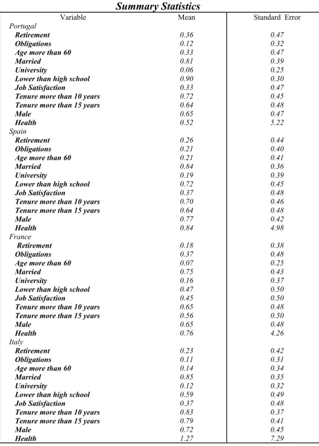
Note that the last variable, which we used as a proxy for the worker’s obligations, tells us that the greater the household debts, the higher will be the workers’ obligations. Now, as this variable takes value 1 if any member of the household is currently paying any debt and 0 otherwise, we expect it to have a negative sign in the estimation, so that it agrees with the assumption of the model to be developed in the next chapter12. A closer look at the summary statistics in the annex show us that, on average, 12% of the workers from Portugal and Italy have to repay debts, while this value grows to 21% if we consider only the Spanish workers. We can also see that Italy is the country that presents the lowest level of obligations, while France is the one that presents the highest.

9

In this way, we can see the present empirical exercise as an analysis of a particular segment of the labor market to a situation where every worker has the right to retire.

10

Note that, with this strategy, we can identify all individual characteristics near the worker’s entry into retirement decisions.

11

As Spanish and Italian legislation did not define, between 1994 and 1999, any maximum age of retirement, we considered the same age as Portugal, 70 years.

12

(5)

To obtain the information related to the effect of worker’s health over his retirement decisions, we consider the question in the ECHP related to the number of nights spent in hospitals during the last 12 months. The reason to include this last variable is that the model needs to capture the effects of the worker’s health over his retirement decision. We can expect that the greater the number of nights spent in hospital, the more probable it is that the worker decided to retire due to poor health. Another look at the summary statistics shows us that the Italian workers spent the greatest number of nights in hospitals, while the Portuguese workers were those who spent the lowest number of nights in the 12 months prior to retirement.

Regarding the workers’ education, marital status and age, which are all important to control for the basic workers’ characteristics, we consider: a dummy variable that equals one if the worker has finished the third level education and zero otherwise; a dummy variable that equals one if the worker has finished less than the second stage of the secondary education and zero otherwise; a dummy variable that equals one if the worker is married and zero otherwise; and a dummy variable that equals one if the worker was more than 60 years old and zero otherwise.

The summary statistics show us that Portugal is the country that has the lowest number of workers who finished third level education, only 6%, while Spain is the country that has the greatest, 19 % of workers. We can also see that Portugal is the country that has the highest number of workers with less than the second stage of the secondary education, 90%, while France is the country that has the lowest, 47%. In all countries the number of married workers is around 82%, while the number of workers older than 60 years is between 7 % for France and 33% for Portugal.

Finally, we also considered the worker’s tenure and the satisfaction with his present job. Both variables were included in order to capture the effects of the quality of the job over the worker’s retirement decision. Now, the greater the job satisfaction, the more will be the worker’s commitment to the job, we expect the relationship between the worker’s satisfaction with his present job and his retirement decision to be negative.

B – Econometric Model

In order to analyze the relationship between obligations and the worker’s exit from the labor force we estimated the latent variable model:

(1) y*_{i t}_, =x_{i t}_,β+c_i+e_{i t}_, ,

where y*_{i t}_, is a binary non-observable variable, which takes value one if the worker decides to retire and zero otherwise, x_{i t}_, is a vector of individual characteristics, c_i

represents non-observable and fixed individual characteristics, and e_{i t}_, represents an error term.

Note from the last expression that as we do not observe * , i t

y , but only the signal of

* , i t

y , it is considered that y_{i t}_, =1, if * , 0 i t

y > , and y_{i t}_, =0, if * , 0 i t y ≤ .

(6)

normal distribution with linear expectations and constant variance are considered in the random effect probit model13.

C – Results

We initially estimate three different models for each country. Two probit models differing only in the vector of covariates, and a random probit model. In the first probit model we consider only the worker’s obligations as independent variable, while in the second we consider other covariates. The third and final estimated model is simply a random probit version of the more complete probit model. In table 4.1 we show these three models for the whole sample and table 4.2 and 4.3 present the results for the male and female sub-samples.

The estimated coefficients, together with their standard errors, are given in the tables below.

TABLE 1

Estimation Results – General

Countries Variables

Probit Probit Random Probit

France

Constant Obligations Married

Lower than high school Age more than 60 Health

Tenure more than 15 years Job Satisfaction

Number of Observations Likelihood Ratio Test Statistic

Italy

Spain

Constant Obligations Married University

Tenure more than 10 years Number of Observations Likelihood Ratio Test Statistic

Portugal Constant Obligations -0.84(0.062)* -0.24(0.108)** -832 5.04 -0.72(0.031)* -0.14(0.100) -2111 2.11 -0.62(0.032)* -0.14(0.072)*** -2239 3.64 -0.34(0.028)* -0.23(0.084)* -0.89(0.144)* -0.20(0.113)*** -0.22(0.120)*** 0.23(0.108)** 1.25(0.184)* 0.01(0.013) -0.05(0.107) -0.06(0.109) 832 67.54 -0.97(0.121)* -0.10(0.106) -0.10(0.089) 0.10(0.068) 1.46(0.085)* 0.01(0.004) 0.08(0.081) -0.13(0.068)*** 2111 334.02 -0.55(0.085)* -0.13(0.072)*** -0.17(0.077)** -0.15(0.075)** 0.15(0.064)** 2239 16.80 -0.38(0.113)* -0.22(0.085)* -1.03(0.190)* -0.23(0.138)*** -0.26(0.151)*** 0.27(0.136)*** 1.38(0.226)* 0.01(0.015) -0.03(0.133) -0.10(0.137) 832 49.54 -1.02(0.134)* -0.10(0.113) -0.12(0.098) 0.10(0.074) 1.52(0.097)* 0.01(0.004) 0.74(0.088) -0.14(0.074)*** 2111 256.64 -0.71(0.118)* -0.12(0.089) -0.20(0.107)** -0.17(0.103)*** 0.19(0.086)** 2239 12.01 -0.62(0.182)* -0.24(0.120)** 13

(7)

Married

Lower than high school Tenure more than 15 years Job Satisfaction

-2416 7.78 -0.25(0.066)* 0.25(0.093)* 0.14(0.055)* -0.21(0.058)* 2416 52.78 -0.38(0.110)* 0.44(0.148)* 0.21(0.090)** -0.26(0.081)* 2416 42.18

Note: *,** and *** represent significance at levels 1, 5 and 10% , respectively. We also tested other variables, such as household size, job status, number of employees in the current job and job sector, but all were strongly non-significant. For the Random Probit Model the presented statistic is not the Likelihood Ratio Test Statistic but the Wald Test Statistic. Standard errors in parenthesis.

TABLE 2

Estimation Results – Males

France

Italy

Spain

Portugal

-0.90(0.080)* -0.20(0.134) -543 2.15 -0.65(0.037)* -0.24(0.120)** -1515 4.25 -0.62(0.036)* -0.19(0.084)** -1718 5.14 -0.30(0.034)* -0.28(0.106)* -1585 6.94 -0.78(0.210)* -0.13(0.140) -0.31(0.170)*** 0.18(0.137) 1.25(0.264)* 0.02(0.016) -0.01(0.138) -0.15(0.139) 543 34.01 -0.94(0.157)* -0.20(0.129) -0.10(0.127) 0.12(0.079) 1.39(0.095)* 0.01(0.004) 0.09(0.094) -0.15(0.079)*** 1515 251.41 -0.65(0.121)* -0.18(0.084)** -0.11(0.112) -0.08(0.087) 0.18(0.076)** 1718 12.26 -0.31(0.161)** -0.24(0.107)** -0.27(0.099)* 0.27(0.128)** 0.12(0.068)*** -0.27(0.070)* 1585 40.17 -0.89(0.263)* -0.17(0.165) -0.34(0.206)*** 0.19(0.165) 1.30(0.301)* 0.02(0.018) -0.01(0.166) -0.18(0.168) 543 26.30 -0.97(0.172)* -0.20(0.136) -0.10(0.140) 0.12(0.086) 1.45(0.110)* 0.01(0.005) 0.08(0.103) -0.16(0.086)*** 1515 189.60 -0.89(0.180)* -0.20(0.105)** -0.08(0.166) -0.06(0.123) 0.23(0.105)** 1718 8.82 -0.45(0.245)*** -0.24(0.143)*** -0.37(0.154)** 0.37(0.191)*** 0.17(0.107) -0.30(0.096)* 1585 26.48

(8)

TABLE 3

Estimation Results – Females

France

Italy

Spain

Portugal

-0.75(0.101)* -0.31(0.186)*** -289 2.89 -0.93(0.064)* -0.12(0.179) -596 0.47 -0.59(0.066)* 0.02(0.145) -521 0.01 -0.40(0.048)* -0.15(0.141) -831 1.20 -0.96(0.208)* -0.29(0.200) -0.15(0.193) 0.27(0.192) 1.33(0.280)* -0.05(0.054) -0.16(0.187) 0.09(0.184) 289 37.00 -0.96(0.218)* 0.16(0.191) -0.23(0.140)*** 0.01(0.132) 1.62(0.199)* -0.01(0.024) 0.04(0.161) -0.12(0.141) 596 80.94 -0.47(0.131)* 0.04(0.146) -0.20(0.121)*** -0.35(0.155)** 0.11(0.128) 521 8.83 -0.44(0.167)* -0.15(0.143) -0.33(0.096)* 0.19(0.137) 0.19(0.096)** -0.09(0.102) 831 20.19 -1.14(0.301)* -0.34(0.252) -0.20(0.252) 0.33(0.251) 1.54(0.389)* -0.06(0.063) -0.15(0.239) 0.04(0.239) 289 21.43 -0.96(0.218)* 0.16(0.191) -0.23(0.140)*** 0.01(0.132) 1.62(0.199)* -0.01(0.024) 0.04(0.161) -0.12(0.141) 596 72.94 -0.59(0.178)* 0.07(0.177) -0.26(0.163) -0.42(0.205)** 0.19(0.170) 521 7.39 -0.75(0.298)* -0.24(0.216) -0.57(0.179)* 0.44(0.245)** 0.31(0.174)** -0.30(0.157)** 831 19.73

Note: *,** and *** represent significance at levels 1, 5 and 10% , respectively. We also tested other variables, such as household size, job status, number of employees in the current job and job sector, but all were strongly non-significant. For the Random Probit Model the presented statistic is not the Likelihood Ratio Test Statistic but the Wald Test Statistic. Standard errors in parenthesis.

We can observe from the three models in Table 4.1 that the worker’s obligations affect negatively, and in a significant way, the probability of workers from France, Spain and Portugal going to retirement. We obtain a similar result for Italy, although it is statistically non-significant in all three models.

(9)

From the university and lower than high school variables we can observe that the higher the education level, the lower is the probability of going to retirement. A possible justification for this could be that the lower the worker’s education, the more probable it is that we will find him working in a more physically demanding job, a factor that could positively affect his entry into retirement.

The worker’s satisfaction with his present job also affects in a negative and significant way the probability of the Portuguese and Italian workers exiting the labor force. An opposite result gives us the worker’s tenure in Italy, Spain and Portugal, demonstrating that the higher the worker tenure, the higher will be his probability of exiting the labor force14.

We can observe from Table 4.2 that the male estimations give us very similar results. The only difference is found in the statistical significance of some variables. On one hand, we can observe an increase in the significance level of some variables, as is the case of the Italian male. On the other hand, we can also see a reduction in the significance level of some variables, as is the case of France and Portugal.

Table 4.3 gives us a different picture. First, we can observe from the estimated models for Italy and Spain that there is an opposite sign for the effect of the workers’ obligations over their retirement decisions. However, we can also note from these estimations that all these results are not statistically significant.

Another difference among the female and the other two estimated models is found in the significance levels of some variables. However, and contrary to the previous analysis, we can now see a generalized decrease in the significance levels of some variables of the models.

3. Theoretical Model

We saw in the previous section that the greater the worker obligations, the lower will be his probability of going to retirement. In this section we will develop a theoretical model intending to evaluate the aggregate effects of this workers’ strategy.

Suppose that our economy is composed of a constant population of workers who live infinitely and a great number of firms that once together, one by one, give rise to a productive activity. Every worker has the right to go to retirement15. Firms and the workers are risk neutral and discount the future at the exogenous and constant rater. Before the beginning of production, firms and workers are involved in a search process to find a partner, where c represents the cost of the search for the firm. The occupied jobs produce x at each instant of time and can be destroyed due to an idiosyncratic shock that follows a Poisson Process with arrival rateλ. The number of job matches formed per period is given by a non-negative, concave, homogeneous of degree one and increasing in both arguments function m v u

(

,

)

, where v represents the vacancy rate and u the fraction of unemployed workers in the economy.

The unemployed workers move to an employed situation at a rate θq

( )

θ , while a job vacancy moves towards a filled position according to a rate q

( )

θ , where θ represents the ratio of v and u.

14

We obtain a different signal for France, although it is statistically non-significant.

15

(10)

Each firm has only one job position, which can be empty or occupied, while each worker can be retired (having he decided to go to retirement), unemployed or employed in only one job position per period. Workers can go immediately to retirement or postpone, at no cost, their exit from the labor force. Suppose that this decision depends only on the exogenous level of workers’ obligations,ο. However, once the worker has decided to retire he cannot return to the labor force.

At each moment there is a change in the worker’s obligation, determined from a general distributionG

( )

ο , defined in the unit interval. Suppose that ο affects positively the value of employment and unemployment and that each firm knows neither the level of workers’ obligations, considering that they move to retirement at rateϕ, nor the effects of obligations over their decision of entry into retirement16. We are therefore considering that there are events that change the level of a worker’s dependence on the employed and unemployed conditions, postponing his exit from the labor force, and that the firm does not take this movement into account, considering that workers enter into retirement at a rate ϕ.

Let S and T represent, respectively, the reservation obligations of the employed and unemployed worker17. Suppose that V and J represent both the values of a vacancy and an occupied job to the firm, while U , W and R represent the values of unemployment, employment and retirement to the worker. Accordingly, the value functions for the firm and the worker are given by:

(2) rV = − +c q

( )

θ

[

J−V

]

;

(3) rU =Max z

{

+θ θq

( )

[

W−U

]

;rR−ο

}

; (4) rR= −y dR;

(5) rW =Max w

{

−λ_W−Max U R

(

,

)

_;rR o−

}

(6) rJ = − −x w λ

[

J−V

]

−ϕ

[

J−V

]

;

where z represents the unemployment insurance benefits, y the retirement benefits,

d the rate that the retired worker leaves this condition and w the worker’s wage rate18.

We can see from these expressions and the above assumptions about S and T_that

the worker evaluates the employment and unemployment options according to his obligations. Thus, whenever ο >S (ο >T) the employed (unemployed) worker postpones his entrance into retirement. In turn, whenever ο≤S (ο≤T) the employed (unemployed) worker decides to go to retirement19. Note also that once the decision to go to retirement is postponed, the worker remains in the labor force until his obligation is reduced to a value below S or T.

We can also observe from expressions (2), (4) and (6) that they are not affected by the worker’s obligation, as the only reason for their presence in the model is to create

16

Observe that the right to retire affects positively the employment and unemployment options due to the increase in the worker’s outside option that it creates.

17

Note that S(T) represents the indifference obligations’ level between employment (unemployment) and retirement.

18

Note that once in retirement, the only way to abandon this situation is at rated.

19

(11)

pressure on the worker’s decision to retire, and from (5) that once an idiosyncratic shock occurs, the worker decides whether to go to unemployment or retirement. Also note from the previous expressions that we are modeling a situation where the worker values differently from the firms, and without knowledge of them, their options. If we eliminate this previous condition, we would have the firm knowing the right rate that the workers leave the labor force, that is, we would have G S

( )

=ϕ. Accepting the usual hypothesis of free entrance, we have from (2) that

(7) . ( )

c J

qθ

=

Thus, there is job creation up to the point where the value of a new job matching equalizes the cost of occupying a vacancy, expressed in terms of the rate that this position becomes occupied.

If the surplus generated by the matching is divided according to the Generalized Nash

Bargaining Solution,then the wage rate satisfies20:

(8) β

[

J−V

]

=

(

1−β

)

_W −Max U R

[

,

]

_.

Using expressions (2) – (8), the wage rate is given by21:

(9)

( )

(

1

)

(

)

c y

w x

q r d

ϕ

β β

θ

 

= _ − _+ −

+

  , if R≥U

( )

(

1

)

c

w x c z

q

ϕ

β θ β

θ

 

= _ + − _+ −

  , if R<U .

Note that they are both composed of two terms. From the first expression, the first term is related to the worker’s productivity in his current job and to the expected search cost, given the worker’s decision to go to retirement; while the second term is related to the retirement benefits. From the second expression, the first term is related to the worker’s productivity in his current job, the average search cost and the expected search cost, given the worker’s decision to go to retirement; while the last is related to the unemployment insurance benefits.

Note from both expressions that they do not depend on the worker’s obligations, since the firm does not know its effects over the worker’s entrance into retirement; that the worker’s wage rate diminishes with the right to retire, and that the higher the probability of the worker’s entrance into retirement, in the firms’ perspective, the lower will be his wage rate22.

20

See Binmore, Rubinstein and Wolinsky (1986) concerning the use of Nash Bargaining in job search models. The termβ represents the worker’s bargaining power.

21

Note from (8) that

(1 )

W U β J

β = +

− . Using this expression in the left-hand side of (5), together

with (3) and (6), we obtain (9).

22

(12)

Note from the first expression that the greater the production generated by the job matching, the retirement benefits, the worker’s bargaining power and the lower the market tightness, the higher will be the worker’s wage rate.

The wage rate increases with reductions in the market tightness because the firm deducts from the worker’s wage rate the effect that his entry into retirement generates to the firm – search costs to find another unemployed worker. The higher the market tightness, the more easily a firm with a vacancy can find an unemployed worker; the lower will be the wage penalization, and the higher will be the worker’s wage rate. Continuing the equilibrium characterization, suppose that:

(10) z

( )

ο = +z ο and (11) w

( )

ο =w+ο,

represent, respectively, the wage and the unemployment benefits compatible with the employed and unemployed worker’s obligations.

Using this definition, suppose that (3) and (5) are given by

(12) rU

( )

ο =Max z

{

( )

ο +θ θq

( )

_W

( )

ο −U

( )

ο _;rR

}

;

(13) rW o

( )

=Max w o

{

( )

−λ_W o

( )

−Max U o R_

( )

, __,rR

}

.

Now, as in the indifference levels S and T, we have that: (14) W S

( )

=R,

(15) U T

( )

=R,

then, evaluating (12) and (13) at T and S, together with the expression (4), we have that:

(16)

( )

(

) ( )

( ) 1

ry c

w S

d r q

βλ

β θ

= +

+ − ,

(17)

( )

(

)

( ) 1

ry c

z T

d r

β θ β

= −

+ − ,

represent the wage rate and unemployment insurance benefits compatible with the indifference obligation.

Note that expression (16) ((17)) tells us that there is an w S

( )

(z T

( )

) that makes the worker indifferent between employment and retirement (unemployment and retirement) options.

Note from (16) that the greater are y, r, β, λ and θ, or the less is d, the higher is the wage that the worker wishes to receive, given his obligations, in order to be indifferent between going or not to retirement. In this manner, we can expect that economies with larger retirement benefits, or higherθ, will have a higher flow of workers from employment to retirement23. In turn, we have from (17) that the larger are y and r, or the lower are d, θ and β, the greater must be the unemployment

23

(13)

insurance benefits to be compatible with the indifference between the unemployment and retirement options.

The entry into retirement increases with reductions in the market tightness basically because firms deducts from the worker’s wage rate the effect that his entry into retirement generates to the firm – search costs to find another unemployed worker. In this way, the higher is θ, the lower is the incentive to postpone retirement.

Now, as we consider that in indifference the worker decides to go to retirement, then whenever the wage rate and the unemployment benefits compatible with his obligations are given by (16) and (17), the employed and unemployed worker will leave the labor force. In turn, if the wage rate (unemployment insurance benefits) compatible with his obligations is higher than w S

( )

(z T

( )

), we will have the worker postponing his entry into retirement.

Proposition 1 It is necessary that y>z

( )

ο , in order to have flows of workers from unemployment to retirement. In turn, it is not necessary that y>w

( )

ο to have flows of workers from employment to retirement.

Proof. We need only to use (16) and (17) and consider a general level of obligations to demonstrate proposition 1.

The previous proposition tells us that it is necessary to compensate the unemployed worker, apart from the term related to the unemployment insurance benefits, with an amount related to the gains that the unemployed worker obtains when finding a new vacancy and moving into an employed status, for there to be a flow of workers from unemployment to retirement. Thus, if the unemployed worker is not correctly compensated, he will not be motivated to exercise his right to retire.

The same cannot be said about the employed worker because even when reducing his retirement pension to an amount below w

( )

ο , it still may not be enough to eliminate the flow of workers from employment to retirement.

Having determined the entry into retirement dynamics, given worker’s obligations, we will now see the optimal job creation rule. From expression (6), we have that:

(18)

[

]

( )

c

r x w

q λ ϕ

θ

+ + = − .

In this we have that the higher is the rate that the worker goes to retirement (in the firm’s perspective), the lower will be the rate of job creation; and that the older is the labor force (closer to obtain the right to retirement), the lower will be the job creation dynamics24. Note also that the higher are r,λ, c and x, or the lower is w, the lower will be the job creation rate.

Another thing that we can observe is that if ϕ is higher than the rate at which the worker effectively requests his right to retire, the right to retire drives a reduction in the job creation flow when compared to the model where G S

( )

=ϕ. Thus, the ignorance of the exact rate whereby the worker goes to retirement could severely penalize the job creation dynamics.

24

(14)

Now, supposing that b measures the rate at which workers enter into the labor force25, the unemployment rate dynamic is given by:

(19) u• =λ_1−G T

( ) (

_ 1− −u a

)

+ −b θ θq

( )

u G T u−

( )

,

where the first term on the right-hand side represents the flow of workers who move to unemployment due to the idiosyncratic shock, the second term represents the number of workers who enter the labor market via unemployment, the third term represents the number of unemployed workers who move to the employment condition, and the last gives us the number of unemployed workers who move to retirement.

Now, as in the steady rate u 0

•

= , then:

(20)

( ) (

)

( )

1 1

1

G T a b

u

G T q G T

λ

λ θ θ

− − +

 

 

=

− + +

 

  ,

represents the equilibrium unemployment rate.

Note that if the number of new unemployed workers rises or if the probability of the unemployed workers going into retirement falls, the result will be an increase in the equilibrium unemployment rate.

The idea behind this latter effect is that the lower is T, the greater is the probability of an unemployed worker not to request his right to retire, increasing the unemployment rate. In turn, the higher is the market tightness or the retirement rate, the lower will be the unemployment equilibrium rate.

Continuing the equilibrium characterization, we have that:

(21) a G T u G S

( )

( )(

1 u a

)

da λG T

( )(

1 u a

)

•

= + − − − + − − ,

is the expression that determines the equilibrium rate of retirement. The first term on the right-hand side gives us the number of unemployed workers going to retirement, the second gives us the number of employed workers who decide to go to retirement, the third represents the number of retired workers who leave this status and the last represents the number of workers who move to retirement due to the idiosyncratic shock.

Considering also the steady state condition, we have that:

(22)

( )

(

) ( )

( )

1

G S G T u G T G S

a

G S d G T

λ λ

λ

+ + − −

   

   

=

+ + ,

gives us the equilibrium retirement rate.

25

(15)

We can observe from this expression that whenever G S

( ) (

> 1−λ

) ( )

G T the increase in the equilibrium unemployment rate comes with a decrease in the retirement rate. In turn, if G S

( ) (

< 1−λ

) ( )

G T , we will have the opposite effect.

Increases in G S

( )

will be followed by an increase in the retirement rate if

(

1−u d

)

>uG T( ), while if

(

1−u d

)

<uG T( ), we will have the opposite effect. In turn, increases in d and decreases in G T( ) will be accompanied by reductions in a.

Proposition 2 The job creation condition (18) and the job destruction condition (16) uniquely determine the equilibrium values of θ and w S

( )

.

Proof. As the job destruction condition is increasing in θ - w S

( )

space, while the job creation condition does not depend on w S

( )

, the equilibrium exists and is unique. Knowing the equilibrium values of θ and w S

( )

, expressions (9), (17), (20) and (22) determine the equilibrium values of w, z T

( )

, u and a.

Now, note that the main characteristics of the model are obtained from the expressions that determine the job creation and job destruction dynamics, the unemployment and the retirement rate. An increase in the retirement benefit, for example, will be followed by increases in w S

( )

, z T

( )

and no changes in the job creation dynamics. Now, as G S

( )

and G T

( )

increase, the overall effect over unemployment and retirement rates will depend on the magnitude of these two movements.

Note also that increases in ϕ come with reductions in θ. Now, as θ decreases we will again have two effects acting over the unemployment and retirement rates. On one hand, the reduction in w S

( )

comes with a reduction in a, due to the lower employed entrance rate into retirement, and an increase in u. But on the other hand, the increases in z T

( )

come with an increase in a, due to the higher unemployed entrance rate into retirement, and a reduction in u. The overall effect will depend on these two opposite effects.

4. Conclusions

The goal of this chapter was to study the effects of higher obligations level over the optimal entrance of workers into retirement.

(16)

5. References

ANDERSON, K. H. BURKHAUSER, R.U. and QUINN, J.F. (1986), “Do Retirement Dreams Come True? The Effect of Unanticipated Events on Retirement Plans”, Industrial and Labor Relations Review, 39(4), July, 518-526.

BANCO DE PORTUGAL, (2004), “Relatório de Estabilidade Financeira”.

BERNHEIM, B.D., SKINNER, J. and WEINBERG, S. (1997), “What Accounts for the Variation in Retirement Wealth Among U.S. Households?”, NBER, Working Paper 6227.

BHATTACHARYA, J., MULLIGAN, C.B. and REED III, R.R. (2004), “Labor Market Search and Optimal Retirement Policy”, Economic Inquiry, 42 (4), October, 560-571.

BINMORE, K., RUBINSTEIN, A. and WOLINSKY, A. (1986), “The Nash Bargaining Solution in Economic Modeling”, Rand Journal of Economics, 17, 166-188.

BOUND, J., SCHOENBAUM, M. and WAIDMAN, T. (1995), “Race and Education Differences in Disability Status and Labor Force Attachment in the Health and Retirement Study”, The Journal of Human Resources, 30, 227-267.

BROWNING, M. and LUSARDI, A. (1996), “Household Saving: Micro Theories and Micro Facts”, Journal of Economic Literature, XXXIV, 1797-1855.

BURTLESS, G. (1986) “Social Security, Unanticipated Benefit Increases, and the Timing of Retirement”, Review of Economic Studies, 53(5), October, 781-805.

CAVALCANTI, T. (2004), “Layoff Costs, Tenure, and the Labor Market”. Economics Letters, 84, 383-390.

DIAMOND, P.A. and HAUSMAN, J.A. (1984), “Individual Retirement and Savings Behaviour”, Journal of Public Economics, 23, 81-114.

ESCHTRUTH, A. and GEMUS, J. (2002), “Are Older Workers Responding to the Bear Market”, Center for Retirement Research, Boston College, September, Number 5.

ENGEN, E.M., GALE, W. and UCCELLO, C. (1999), “The Adequacy of Retirement Saving”, Brooking Papers on Economic Activity, 2, 65-165.

EUROSTAT (2003), “European Community Household Panel Longitudinal Users’ Database”. EUROSTAT, DOC. PAN 168/2003-06.

FIELDS, G. S. and MITCHELL, O.S. (1984a), “Economic Determinants of the Optimal Retirement Age: An Empirical Investigation”, Journal of Human Resources, 14, 245-262.

FIELDS, G. S. and MITCHELL, O.S. (1984b), “The Effects of Social Security reforms on Retirement Ages and Retirement Incomes”, Journal of Public Economics, 25, 143-159.

FIELDS, G.S. and MITCHELL, O.S. (1984c), “The Economics of Retirement Behaviour”, Journal of Labor Economics, 2(1), January, 84-105.

FLIPPEN, C. and TIENDA, M. (2000), “Pathways to Retirement: Patterns of Labor Force Participation and Labor Market Exit Among the Pre-Retirement Population by Race, Hispanic Origin and Sex”, Journal of Gerontology, 55(1), 14-27.

GARIBALDI, P. and WASMER, E. (2005), “Labor Market Flows and Equilibrium Search Unemployment”. Journal of the European Economic Association, 3(4), June, 851-882.

(17)

GRUBER, J. and WISE, D. (2005), “Social Security Programs and Retirement Around the World: Fiscal Implications, Introduction and Summary”, NBER, Working Paper 11290.

HURD, M. and ZISSIMOPOULOS, J. (2003), “Saving for Retirement: Wage Growth and Unexpected Events”, Mimeo, Boston College.

JOHNSON, R.W. and NEUMARK, D. (1997), “Age Discrimination, Job Separations, and Employment Status of Older Workers: Evidence from Self-Reports”, Journal of Human Resources, 32, 779-811.

LJUNGQVIST, L. and SARGENT, T. (1998), “The European Unemployment Dilemma”, Journal of Political Economy, 106, June, 514-550.

MORTENSEN, D.T. and PISSARIDES, C.A. (1994), “Job creation and job destruction in the theory of unemployment”, The Review of Economic Studies, 61(July), 733-53.

MORTENSEN, D. and PISSARIDES, C. (1998), “Technological Progress, Job Creation and Job Destruction”, Review of Economic Dynamics, 4, 733-753.

PISSARIDES, C. (2000), “Equilibrium Unemployment Theory”, second edition, MIT Press.

PERACHI, F. and WELCH, F. (2001), “Trends in Labor Force Transitions of Older Men and Women”, Journal of Labor Economics, 12, 210-242.

PRIES, M.J. and ROGERSON, R. (2004), “Search Frictions and Labor Market Participation”, Mimeo, University of Maryland.

QUINN, J. (1977), “Microeconomic Determinants of Early Retirement: A Cross-Sectional View of White Married Men”, The Journal of Human Resources, 12(3), 329-346.

SAAS, S. (2003), “Reforming the U.S. Retirement Income System: The Growing Role of Work”, Center for Retirement Research, Boston College, September, Number 1.

SATTINGER, M. (1995), “General Equilibrium Effects of Unemployment Compensation with Labor Force Participation”, Journal of Labor Economics, 13(4), 623-652.

VERACIERTO, M. (2002), “On the Cyclical Behaviour of Employment, Unemployment and Labor Force Participation”, Working Paper, Federal Reserve Bank of Chicago.

WILLIAMSON, J.B. and McNAMARA, T. K. (2002), “The Effect of Unplanned Changes in Marital and Disability Status: Interrupted Trajectories and Labor Force Participation”, Working Paper 2002-5, Center for Retirement Research, Boston College.

WOOLDRIDGE, J. (2002), “Econometric Analysis of Cross Section and Panel Data”, MIT Press, Cambridge, MA.

(18)

6. Annex

TABLE 4

Description of Variables

Retirement

Obligations

Age more than 60

Married

University

Lower than high school

Job Satisfaction

Tenure more than 10 years

Tenure more than 15 years

Male Health

Variable that takes value 1 if the worker decides to retire in the next period and 0 otherwise;

Variable that takes value 1 if any member of the household is currently paying any debt and 0 otherwise;

Variable that takes value 1 if the worker is more than 60 years old and 0 otherwise;

Variable that takes value 1 if the worker is married and 0 otherwise;

Variable that equals 1 if the worker has finished a third level education and 0 otherwise;

Variable that equals 1 if the worker has finished less than the second stage of secondary education and 0 otherwise;

Variable that equals 1 if the worker is satisfied with his job and 0 if not satisfied;

Variable that equals 1 if the worker has tenure of more than 10 years and 0 if not;

Variable that equals 1 if the worker has tenure of more than 15 years and 0 if not;

(19)

TABLE 5

Summary Statistics

Variable Mean Standard Error

Portugal

Retirement Obligations Age more than 60 Married

University

Lower than high school Job Satisfaction

Tenure more than 10 years Tenure more than 15 years Male

Health

Spain

University

Health

France

University

Health

Italy

University