A comparison between Joint Regression Analysis and the Additive Main and Multiplicative Interaction model: the robustness with increasing amounts of missing data

Note

A comparison between Joint Regression Analysis and the Additive

Main and Multiplicative Interaction model: the robustness with

increasing amounts of missing data

Paulo Canas Rodrigues

1

*, Dulce Gamito Santinhos Pereira

2

, João Tiago Mexia

1

1_{Universidade Nova de Lisboa/Faculdade de Ciências e Tecnologia/CMA – Depto. de Matemática – 2829-516 – Caparica,}

Portugal.

2_{Universidade de Évora /Colégio Luís António/CIMA – Depto. de Matemática, Rua Romão Ramalho, 59 – 7000-671 – Évora,}

Portugal.

*Corresponding author <paulocanas@fct.unl.pt> Edited by: Marcin Kozak

ABSTRACT: This paper joins the main properties of joint regression analysis (JRA), a model based on the Finlay-Wilkinson regression to analyse multi-environment trials, and of the additive main effects and multiplicative interaction (AMMI) model. The study compares JRA and AMMI with particular focus on robustness with increasing amounts of randomly selected missing data. The application is made using a data set from a breeding program of durum wheat (Triticum turgidum L., Durum Group) conducted in Portugal. The results of the two models result in similar dominant cultivars (JRA) and winner of mega-environments (AMMI) for the same environments. However, JRA had more stable results with the increase in the incidence rates of missing values.

Keywords: AMMI models, genotype by environment interaction, joint regression analysis, missing values, durum wheat

Introduction

Joint Regression Analysis (JRA) has been widely used in crop sciences, to structure and understand Genotype by Envi-ronment Interaction (GEI) (Eberhart and Russell, 1966; Finlay and Wilkinson, 1963; Gusmão, 1985; Mooers, 1921; Pereira and Mexia, 2008; Yates and Cochran, 1938; Zheng et al., 2009), and in genetics, to analyse quantitative trait loci (QTL) by environ-ment interaction (Emebiri and Moody, 2006; Korol et al., 1998). In this paper we are mainly interested in the approach proposed by Gusmão (1985) in which the precision in analysing series of randomized block experiments was highly increased, by con-sidering environmental indexes for individual blocks instead of only one environmental index per experiment. In the literature some variants of JRA are also denoted as SREG (Sites Regres-sion) model (Cornelius et al., 1992; Crossa et al., 2002; Setimela et al., 2007).

Williams (1952), Gollob (1968), Mandel (1971), Bradu and Gabriel (1978) and Gauch (1988) have made an important contribution to the development of additive main effects and multiplicative interaction (AMMI) models. These models have been widely used to analyze multi-environment trials because of their flexibility in allowing the use of several multiplicative terms to explain the GEI. One of the difficulties in choosing the right tool to analyse multi-environment trials arises when there are missing values in the two-way table of genotypes and environ-ments. These missing values can be either systematic (Calinski et al., 1992; Denis and Baril, 1992), or selected completely at random in the two-way table.

This paper brings together the main features of JRA and AMMI models, and compares them for analyzing a durum wheat (Triticum turgidum L., Durum Group) trial with particular focus on robustness with increasing amounts of random

miss-ing data, either missmiss-ing replications or missmiss-ing cells (more likely when the proportion of missing values is high). The aim here is not to compare the method’s ability to estimate missing values in comparison to real data (Alarcón et al., 2010; Bergamo et al., 2008) but to compare the overall stability when increasing the incidence rate of missing values. An emphasis is made in the comparison between (i) the upper contour of JRA and the mega-environments of the AMMI model; and (ii) the stability of the dominant/winner genotypes across environments. To obtain the results for the JRA we developed an R code, and the MATMODEL software (Gauch and Furnas, 1991) was used to fit the AMMI models.

Materials and Methods

Joint regression analysis

JRA has proven to be an important model for analysing and interpreting the GEI of two-way classified data tables and continues to be largely used as a complement of traditional statistical analysis in genetics, plant breeding, and agronomy, for determining yield stability of different genotypes or agronomic treatments across environments (Crossa, 1990). JRA may also be used for the analysis of series of experiments in genotype com-parison and selection. This technique is based on the adjustment of a linear regression, per genotype, of the yield on a synthetic variable measuring productivity, the environmental index.

environments). The model used for the analysis of multi-envi-ronment variety trials can be defined as

(1)

(3)

(4) (2) where μ is the grand mean, Gi and Ej are the genotype and environment main effects, (GE)ij is the interaction and εij is the residual. A sub-model of (1), aiming at estimating some stability parameters for making comparisons between varieties is given by JRA, and allows us to partitioning the GEI into two parts of interest, i.e.

where b_i is a linear regression coefficient for the i-th genotype and δij a deviation (unexplained GEI) (Freeman, 1973). The JRA model can then be written as

where εij comprises both the unexplained GEI and the ex-perimental error (Shukla, 1972). We assume fixed genotypic and environmental effects and random residual term.

The model (3) used in the present paper does not take into account the block effects since it uses the blocks as environ-ments, following Gusmão (1985). If an experiment is designed with randomized blocks and the treatments correspond to the J genotypes to be compared, for each block in each design, the environmental index is measured by the average yield. For each of the J genotypes, a linear regression of yield on environmental indexes is adjusted.

Zamir, 1979; Gauch and Zobel, 1990). For the complete case, Pereira and Mexia (2010) presented an alternative algorithm, the double minimization algorithm, which converges to the absolute minimum of the goal function (4) and is an adaptation of the algorithm first presented by Fisher and Mackenzie (1923). More details on the zigzag and double minimization algorithms can be found in Pereira and Mexia (2010).

Upper contour

When two of the regressions on genotypes intersect it means that one of the genotypes is better for higher mental indexes while the other is preferable for lower environ-mental indexes. The intersection of regressions shows more than one genotype with similar performance. The upper contour

L2 environmental indexes

For convenience, let us consider the joint regression model

of the second equation in (3), where , Ej,

j = 1, ... b, is the environmental index corresponding to blocks instead of environments, b the number of blocks, Y_ij is a con-tinuous response (e.g. yield) for cultivar/genotype i in block j

if present, and the pairs , i = 1,..., I, are the regression coefficients, for the I genotypes.

To obtain the estimates for the regression coefficients and the environmental indexes, the goal function to be mini-mized should be

Usually the weight p_ij is 1 [0] when genotype i is pres-ent [abspres-ent] in block j. These weights may differ from block to block to express differences in representativeness of the blocks and thus we take p_ij = p_j when the i-th genotype is pres-ent. The main problem in such modeling is how to estimate the parameters. However, the lately proposed so called zigzag algorithm (Pereira and Mexia, 2010) is very efficient in finding the estimates of (Gi

*

,bi *

), i =1,...,I,and Ej, j = 1,…b. This zigzag algorithm is an alternating least squares based algorithm (Calin-ski et al., 1992; Denis and Baril, 1992; Digby, 1979; Gabriel and

Figure 1 – Upper contour with the four dominant genotypes in the durum wheat population. The abbreviations for the 11 environments are placed in the axis of the environmental indexes (Bej1: Beja1; Bej2: Beja2; Ben1: Benavila1; Ben2: Benavila2; Evo: Évora; Elv1: Elvas1; Elv2: Elvas2; Elv3: Elvas3; Rev: Revilheira; Tav1: Tavira1; Tav2: Tavira2).

Ockham's hill

overfit noise

underfit

signal _actual

data best model

0.0 0.4 0.8 1.2 1.6 2.0

0 1 2 3 4 5 6 7 8

AMMI model family

st

a

ti

st

ica

l e

ff

ici

e

n

cy

Figure 2 – Ockham's hill for accuracy of the yield estimates for the durum wheat experiment. The abscissa shows AMMI models of increasing complexity from AMMI0 to AMMI8, and the ordinate shows the number of in-direct replications determined by jackknife resampling (e.g. the parsimonious AMMI2 model extract 1.66 time more information than the full AMMI8 model).

6 8 10 12

Y

ield (t

ha

–1)

CELTA

0 2 4

Environmental Index TE9204

TE9008 TE9115

Tav1 Ÿ Ben2

Ÿ Tav2Ÿ

Elv2 Ÿ Elv3Ÿ

Elv1

Ÿ Bej1Ÿ

Bej2 Ÿ Evo

Ÿ Rev

Ÿ Ben1

of the JRA is a concave polygonal (Mexia et al., 1997), consti-tuted by segments of the adjusted regression lines, that contains the higher adjusted yields for the environmental indexes (Fig-ure 1). Each of these segments will correspond to a range of variation of the environmental indexes in which the associated genotype will have the maximum adjusted yield (Pereira and Mexia, 2008). These genotypes are called dominant and should be selected. The remaining genotypes should be compared with the dominant to check whether they are dominated on entire range for the adjusted environmental indexes, [c, d]. If so, they can be safely discarded from the breeding program.

An analogy can be made between Figure 1 in this paper and Figure 2 in Gauch (1997), where the AMMI1 nominal yields for a corn trial is depicted as a function of the environment interaction principal component (IPC) axis 1. A more detailed comparison in what concerns the winner genotypes across the environments is presented latter in this paper.

Genotype comparison and selection

Let L be the number of dominant genotypes with dominant

ranges The entire range for the

environmental indexes will be . To have interac-tion between genotypes and environments there are two possible cases for different slopes, and . After establishing the upper contour, non-dominant genotypes should be compared with the dominant ones. This comparison should be made on the left [right] extreme of the dominance range if the non-dominated genotypes have lower [greater] slope than the dominant one. So, when we are led to compare the adjusted values and at the environmental index . These comparisons between slopes may be made using one of follow-ing statistical tools: (i) one-sided t tests for the null hypothesis; (ii) Scheffé multiple comparison tests (Scheffé, 1959); (iii) Bonferroni multiple comparison method (Seber and Lee, 2003); (iv) Tukey multiple comparison method (only for the complete case); and (v) Control of False Discovery Rate which is robust against erroneous rejections (Benjamini and Hochberg, 1995). More details of these tests can be found in Pereira and Mexia (2008).

AMMI models

The core idea of the AMMI models is: (i) first apply the additive analysis of the variance model (ANOVA) to a two-way data (in the present case with genotypes and environments); and (ii) secondly apply the multiplicative principal component analysis (PCA) model to the residual from the additive model (in this case to the interaction) (Gauch, 1992). The AMMI model with N multiplicative terms can be written as

(ii) to clarify GEI (Crossa et al., 1990; Zobel et al., 1988); and (iii) to improve the accuracy of yield estimates (Crossa et al., 1990; Zobel et al., 1988).

Durum Wheat Yield Data

All the properties and comparisons presented in this paper are illustrated with a data set resulting from a breeding pro-gram in Portugal, carried out by the Portuguese National Plant Breeding Station (ENMP, Elvas) in the years of 1992/1993 and 1993/1994. It contains the yield from nine genotypes (CELTA; HELVIO; TE9006; TE9007; TE9008; TE9110; TE9115; TE9204; and TROVADOR) of durum wheat (Triticum turgidum

L., Durum Group), measured in 11 environments (Benavila1; Revilheira; Évora; Elvas1; Beja1; Tavira1; Elvas2; Tavira2; Elvas3; Benavila2 and Beja2), and performed in complete ran-domized blocks with four replicates. These environments were obtained in two years, the first 6 in the first and the second 5 in the second year. Only the locations Tavira, Benavila and Beja were the same in both years. All the locations in this data set are in south Portugal, Tavira being at the sea side (Algarve) while the remaining in the inland (Alentejo). More details about this data set can be found in Pereira and Mexia (2010).

Simulation of missing values

Since the plants may be destroyed by animals, floods or dur-ing the harvest, and the yield measurements may be erroneously performed and inadequately introduced in the data base, missing values are common in agricultural experiments. When dealing with missing values researchers should decide between: (i) find a good tool to estimate the missing values (Alarcón et al., 2010; Bergamo et al., 2008), or (ii) chose a robust technique against missing observations to perform the analysis. In the present study we will be interested in the second approach, namely to compare the robustness of JRA and AMMI with the increasing of miss-ing data. Our interest here is to study the case where the missmiss-ing values were selected “completely” at random, instead of having systematic patterns (Calinski et al., 1992; Denis and Baril, 1992).

Our simulation procedure can be summarized in the fol-lowing steps:

(i) Choose the incidence rate of missing values α (e.g. α = 5, 10, 25, 50, 75 %);

(ii) Remove, randomly, α % of the two-way table with geno-types and environments, leaving at least one observation in each environment and in each genotype;

(iii) a. Use the zigzag algorithm (Pereira and Mexia, 2010) to compute the regression coefficients and the L2 environmental indexes for JRA by minimizing the loss function (4); Results such as those shown in Figure 1 and in Table 3 can be obtained using the appropriated multiple comparison tests mentioned above. b. Use the MATMODEL software (Gauch and Furnas, 1991) to estimate the missing values; Results such as those shown in Table 3 can be obtained by this software;

(iv) Repeat (ii) and (iii) n times for each incidence rate of miss-ing values. The number of interactions n should be chosen based on the size of the original two-way table. In this particular case we used n=100.

For higher incidence rates of missing values it is more likely that not only replications are missing, but cells (means). (5)

where Y_ij is the yield of genotype i in environment j; μ the grand mean; αi the genotype mean deviations (the genotype means minus the grand mean); β_j the environment mean deviations;

λ

nn the singular value for the PCA axis n;

γ

ni and

δ

nj are the genotype and environment PCA scores for PCA axis n; N is the number of PCA axes retained by the model; and

θ

_ij is the re-sidual. If the experiment is replicated, an error term εijr

,

which

is the difference between the Y_ij mean and the single observation for replicate r, should be added.

In this case an Expectation-Maximization (EM) algorithm provides an effective general strategy for obtaining maximum likelihood estimates (Gauch, 1992). This procedure has been adapted for AMMI and is called EM-AMMI (Gauch and Zo-bel, 1990), and is implemented in the MATMODEL software (Gauch and Furnas, 1991).

Results and Discussion

A comparison between the algorithms and the alternative methods

This subsection presents a comparison between the two algorithms mentioned in the above section - (i) zigzag algorithm (Pereira and Mexia, 2010) and (ii) double minimization algorithm (Pereira and Mexia, 2010); and the two methods based in the joint regression model - (iii) the regression analysis of the mean yield of individual genotypes on the overall mean of the trial (Finlay and Wilkinson, 1963), and (iv) the regression analysis of the genotype mean yield on block mean, proposed by Gusmão (1985). This comparison is illustrated with a numerical example using the durum wheat yield population. Estimates of intercept, slope and the coefficients of determination, obtained from the Finlay and Wilkinson (1963) and Gusmão (1985) methods, and the zigzag and double minimization algorithms are presented in Table 1.

To compare these four procedures it is important to analyze the slopes and coefficients of determination. They produced almost the same results regarding the ordering of the genotypes per slope (only the Gusmão’s method gave a small difference). The coefficients of determination are mainly similar, the zigzag and Double Minimization algorithms being lower than Gusmão (1985) only for three environments (HELVIO, TE9110 and TE9115). Moreover, the zigzag and double minimization have completely agreed and may be seen as the most suited for re-gression analysis of complete randomized blocks because of their convergence to the minimum of the loss function (4).

Another comparison can be made regarding the sums of the sums of squares of residuals for the two procedures and two algorithms (Table 2). Here the advantage of the zigzag and double minimization algorithms over the two other procedures is evident since the algorithms induce lower sums of the sums of squares of residuals. This result is true for all the examples and the mathematical proof can be found in Pereira and Mexia (2010). If we compute the pairwise Pearson correlations be-tween the environmental indexes for the four alternatives in Table 2, we conclude that all the obtained environmental in-dexes are highly correlated (minimum of 0.984). In particular, the results obtained using the zigzag and double minimization algorithms have a coefficient of correlation of 1.000 since they completely agree with each other, and they are slightly bet-ter than the Finlay and Wilkinson (1963) and Gusmão (1985) approaches. In the case of a comparison using α-designs or incomplete blocks (instead of the randomized complete block design) some advantage within the two algorithms could better be presented (Pereira and Mexia, 2010).

Genotype comparison and selection

The results for some of the multiple comparison tests mentioned above can be found in Table 3. The graphical repre-sentation of the dominant genotypes, together with the ranges of dominance (i.e. the lower and upper bound for the interval where the each genotype is dominant) and environments where that dominance occurs, is depicted in Figure 1. The bounds of the environmental indexes 2.21 and 8.84 (Table 3, complete data) are kept unchanged by the zigzag algorithm and corre-spond to the lowest and highest mean yield of all the blocks.

AMMI preliminary analyses

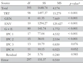
Table 4 gives the ANOVA for AMMI4. The genotypes, en-vironments and GEI account for 4.1 %, 86.4 %, and 9.5 % of the treatment sum of squares (SS). The noise in the GEI may be estimated by the interaction df times the error MS, namely 40.80,

Table 1 – Adjusted regression coefficients and coefficients of determination, as evaluated by the two procedures and two algorithms.

Finlay and Wilkinson (1963) Gusmão (1985) Zigzag and

Double Minimization

Genotype Intercept Slope R2 _{Intercept Slope R}2 _{Intercept Slope R}2

CELTA -0.518 1.239 0.893 -0.472 1.229 0.907 -0.544 1.245 0.918

TE9007 -0.542 1.121 0.907 -0.492 1.110 0.918 -0.544 1.121 0.924

TE9006 -0.300 1.086 0.815 -0.361 1.100 0.863 -0.416 1.112 0.870

TE9204 0.077 1.067 0.861 0.058 1.071 0.895 0.016 1.080 0.899

HELVIO -0.130 1.051 0.902 -0.112 1.047 0.924 -0.244 1.065 0.894

TROVADOR -0.140 1.042 0.841 -0.206 1.056 0.892 -0.154 1.056 0.928

TE9008 0.375 0.951 0.883 0.403 0.945 0.900 0.376 0.951 0.899

TE9110 -0.089 0.892 0.773 -0.051 0.884 0.783 -0.037 0.880 0.767

TE9115 1.268 0.551 0.510 1.232 0.559 0.542 1.297 0.545 0.507

Table 2 – Sums of the sums of squares of residuals, as evaluated by the two procedures and two algorithms.

Finlay and Wilkinson (1963) Gusmão (1985) Zigzag and Double Minimization

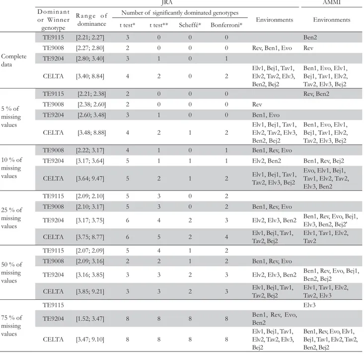
Table 3 – Dominant and number of significantly dominated genotypes for JRA, environments where the genotypes were dominant (JRA) and where the genotypes were winners (AMMI). The results are for the complete data set and the incidence rates of missing values, and based on one run (out of 100) of the simulation described above. Abbreviations for the environments: Bej1: Beja1; Bej2: Beja2; Ben1: Benavila1; Ben2: Benavila2; Evo: Évora; Elv1: Elvas1; Elv2: Elvas2; Elv3: Elvas3; Rev: Revilheira; Tav1: Tavira1; Tav2: Tavira2

JRA AMMI

D o m i n a n t or Winner genotype

R a n g e o f dominance

Number of significantly dominated genotypes

Environments Environments t test* t test** Scheffé* Bonferroni*

Complete data

TE9115 [2.21; 2.27] 3 0 0 0 Ben2

TE9008 [2.27; 2.80] 2 0 0 0 Rev, Ben1, Evo Rev

TE9204 [2.80; 3.40] 3 1 0 1

CELTA [3.40; 8.84] 4 2 0 2

Elv1, Bej1, Tav1, Elv2, Tav2, Elv3, Ben2, Bej2

Ben1, Evo, Elv1, Bej1, Tav1, Elv2, Tav2, Elv3, Bej2

5 % of missing values

TE9115 [2.21; 2.38] 2 0 0 0 Rev, Ben2

TE9008 [2.38; 2.60] 2 0 0 0 Rev

TE9204 [2.60; 3.48] 3 1 0 0 Ben1, Evo

CELTA [3.48; 8.88] 4 2 1 2

Elv1, Bej1, Tav1, Elv2, Tav2, Elv3, Ben2, Bej2

Ben1, Evo, Elv1, Bej1, Tav1, Elv2, Tav2, Elv3, Bej2

10 % of missing values

TE9008 [2.22; 3.17] 4 1 0 1 Ben1, Rev, Evo

TE9204 [3.17; 3.64] 5 1 1 1 Elv2, Ben2 Ben1, Rev, Bej2

CELTA [3.64; 9.47] 5 2 1 2 Elv1, Bej1, Tav1,

Tav2, Elv3, Bej2

Evo, Elv1, Bej1, Tav1, Elv2, Tav2, Elv3, Ben2

25 % of missing values

TE9115 [2.09; 2.10] 5 3 0 2

TE9008 [2.10; 3.17] 5 3 0 2 Ben1, Rev, Evo

TE9204 [3.17; 3.75] 6 4 2 3 Elv2, Elv3, Ben2 Ben1, Rev, Evo, Bej1,

Elv3, Ben2, Bej2'

CELTA [3.75; 8.77] 6 5 2 4 Elv1, Bej1, Tav1,

Tav2, Bej2

Elv1, Tav1, Elv2, Tav2

50 % of missing values

TE9115 [2.07; 2.09] 5 4 1 2

TE9008 [2.09; 3.16] 2 2 1 2 Ben1, Rev, Evo

TE9204 [3.16; 3.85] 3 3 2 3 Elv2, Elv3, Ben2 Ben1, Rev, Evo, Bej1,

Ben2, Bej2

CELTA [3.85; 9.21] 3 3 2 3 Elv1, Bej1, Tav1,

Tav2, Bej2

Elv1, Tav1, Elv2, Tav2, Elv3

75 % of missing values

TE9115 Elv3

TE9204 [1.52; 3.47] 8 8 8 8 Ben1, Rev, Evo,

Ben2

CELTA [3.47; 9.10] 8 8 8 8

Elv1, Bej1, Tav1, Elv2, Tav2, Elv3, Bej2

Ben1, Rev, Evo, Elv1, Bej1, Tav1, Elv2, Tav2, Ben2, Bej2

*0.05; **0.01

which by difference from the total of 141.74 (total GEI SS) im-plies a GEI signal SS of 100.94, or 71.21 % (Gauch, 1992). Fig-ure 2 shows the numbers of indirect replications for the AMMI model family from AMMI0 to AMMI8. The models are less parsimonious, or more complex, moving to the right. AMMI2 achieves the highest number of indirect replications of 1.66 (i.e. 1 replication gives 1.66 more information when considering the parsimonious AMMI2 model). To the left of this model, excessively simple models underfit the real signal, whereas to the right, excessively complex models overfit the spurious noise.

This relationship between accuracy and parsimony has been named as Ockham's hill (Gauch, 2006; Mackay, 1992).

and 38.01 for IPC2), which means that these two PCs are mostly signal whereas the remaining are mostly noise. The F tests in Table 4 also suggested retaining the first two PCs. For com-parison with AMMI, the Finlay-Wilkinson linear regressions on environment mean capture a SS of 43.63, which is about 56.6 % of the GEI SS captured by IPC1.

Figure 3 depicts the AMMI1 biplot for the durum wheat ex-periment. The choice of the AMMI1 biplot instead of AMMI2 was made to allow the comparison with Figure 1. The abscissa shows the main effects and the ordinate shows the IPC1 scores. The 9 genotypes are represented in bold font and the 11 en-vironments in normal font. The first IPC captures 54.73 % (77.04/141.74) of the GEI sum of squares. But, since this GEI is only 71.23 % (100.94/141.74) signal, this graph captures the most of GEI signal and a small amount of noise (Gauch, 1992). With this biplot it is easier to understand the association between genotypes and environments where they perform bet-ter regarding grain yield.

IPC1 makes a distinction between Tavira (Algarve, sea side) and the rest of the environments (Alentejo, inland) (Figure 3). When comparing with Figure 1, we can see that the four domi-nant genotypes are ordered by IPC1 scores in Figure 3. This provides an agreement between the environmental indexes and IPC1 scores, and connects them to a measure of yield produc-tion. The order of environments along the main effects of Figure 3 and environmental indexes of Figure 1 is the same, as expected.

Upper contour and mega-environments

In this subsection we intend to make a comparison between the upper contour of JRA and the AMMI mega-environments (Gauch and Zobel, 1997). Figure 1 shows the 11 environments placed in the axis of the environmental indexes. The first three environments, namely Rev, Ben1 and Evo, have higher yield with the genotype TE9008, and the remaining eight environments have better production with the genotype CELTA.

Follow-ing the same analysis usFollow-ing the AMMI mega-environments as Gauch and Zobel (1997), based on AMMI1 estimates, we may conclude that this data set has three winners: (i) CELTA wins in nine environments; (ii) TE9008 wins in the environment Rev; and (iii) TE 9115 wins in the environment Ben2. However the main conclusion is taken by both analyses: CELTA is the uni-versal winner (Table 3).

Stability with missing values

JRA is an extremely robust technique against missing ob-servations in what concerns genotype comparison and selection (Pereira et al., 2007). They used a series of 17 experiments of

α−designs of winter rye genotypes, in the years of 1997 and 1998, and considered proportions of missing values from 5 % to 75 %, with step size of 5 % generated randomly in triplicate. The durum wheat data set was used here to test the stability and agreement in choosing the dominant genotypes for differ-ent incidence rates of missing values, between JRA and AMMI. Table 3 presents the main results for different incidence rates of missing values. The missing values were chosen randomly as described before.

The analysis of Table 3 should be performed between meth-ods and between incidence rates of missing values. Regarding the comparison between methods, the most similar results are for the complete data without missing values, with eight envi-ronments having higher yield for the same (dominant/winner) genotypes. The number of environments dominated/won by the same genotypes decreases when increasing the proportion of missing values. The only exception is the case with 75 % of missing values, with 6 agreements between analyses, which is more likely to change each time the random procedure to remove observations is run.

Regarding the comparison between percentages of missing values, Table 3 (second, eighth and ninth columns) illustrates a more stable and robust performance of JRA, since the dominant genotypes are kept unchanged for an incidence of missing val-ues until 50 %. While for JRA there are six environments (Rev, Elv1, Bej1, Tav1, Tav2 and Bej2) which are dominated by the Table 4 – AMMI4 analysis of variance. The grand mean is

4.502 t ha–1_.

Source df SS MS p-value*

Total 395 1648.74 4.174

TRT 98 1497.37 15.279 < 0.001

GEN 8 61.35 7.669 < 0.001

ENV 10 1294.27 129.427 < 0.001

G × E 80 141.74 1.772 < 0.001

IPC 1 17 77.04 4.532 < 0.001

IPC 2 15 38.01 2.534 < 0.001

IPC 3 13 10.79 0.830 0.076

IPC 4 11 10.15 0.923 0.052

Residual 24 5.76 0.240 0.985

Error 297 151.37 0.510

Based on F tests. df = degrees of freedom, SS = sum of squares, MS = mean square, TRT = treatments, GEN = genotypes, ENV = environments, G × E = genotype by environment interaction, IPC = interaction principal component.

CELTA

HELVIO TE9006 TE9007

TE9008

TE9110

TE9115

TE9204 TROVADOR

Ben1 Rev

Evo Elv1 Bej1

Tav1

Elv2

Tav2

Elv3 Ben2

Bej2

-2 -1 0 1 2

2 3 4 5 6 7 8 9

Main effects

IP

C

1

same genotypes in all the cases (with exception of the extreme 75 % incidence rate of missing values), for the AMMI analysis it only happens in 4 environments (all of then are won by CELTA). Moreover for the AMMI model the genotype TE9008 and TE9115 only win in one of the five cases (incidence rates), while for the JRA the dominant genotypes are more stable.

Although the dominant genotypes have little change with the incidence rate of missing values it seems clear that CELTA is the strongest genotype regarding the yield production. It is always dominant for higher environmental indexes and always wins one mega-environment. With 75 % of missing values (297 out of 396 observations) the JRA yet identifies two of the dominant geno-types presented in the upper contour of Figure 1, while AMMI identifies a “small” environment Elv3 and a larger mega-environment with the remaining ten mega-environments (Table 3).

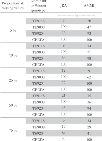
We carried out 100 simulations as described before, and Table 3 shows the results for one of them chosen randomly. The 100 data sets for each proportion of missing values resulted in the identification of, at least, one dominant/winner genotype coincident to the complete data set when considering 75 % of missing values. For 50 % or less JRA always identified TE9008 and CELTA as dominant genotypes, whereas TE9204 (not dominant/winner in the complete data set) and CELTA almost always win one AMMI mega-environment. A detailed summary of the 100 runs is presented in Table 5.

Conclusion

The aim was not to compute estimates of missing values and compare them with the original data, but to compare the final results (i.e. dominant/winner genotypes and environments where the were dominant/winner) between JRA and AMMI and between the complete data and incomplete data sets with different incidence rates of missing values. The main conclu-sions were the similarity between the dominant genotypes in JRA and the winners of the mega-environments in the AMMI analysis; and a more stable performance of JRA for higher pro-portions of missing values. The results from JRA trend to be more significant than those from AMMI models in these kind of trials, because the genotypes in the program have proved to have strong adaptability.

Acknowledgements

Paulo C. Rodrigues acknowledges financial support from Fundação para a Ciência e Tecnologia (Portuguese Foundation for Science and Technology), of Ministério da Ciência, Tecno-logia, e Ensino Superior, Portugal, for doctoral grant SFRH/ BD/35994/2007, and the project N N310 447838 supported by the Ministry of Science and Higher Education, Poland.

References

Alarcón, S.A.; Peña, M.G.; Dias, C.T.S.; Krzanowski, W.J. 2010. An alternative methodology for imputing missing data in trials with genotype-by-environment interaction. Biometrical Letters 47: 1-14.

Benjamini, Y.; Hochberg, Y. 1995. Controlling the false discovery rate: a practical and powerful approach to multiple testing. Journal of the Royal Statistical Society Series B-Methodological 57: 289-300.

Bergamo, G.C.; Dias, C.T.D.S.; Krzanowski, W.J. 2008. Distribution-free multiple imputation in an interaction matrix though singular value decomposition. Scientia Agricola 65: 422-427.

Bradu, D.; Gabriel, K.R. 1978. Biplot as a diagnostic tool for models of 2-way tables. Technometrics 20: 47-68.

Calinski, T.; Czajka, S.; Denis, J.B.; Kaczmarek, Z. 1992. EM and ALS algorithms applied to estimation of missing data in series of variety trials. Biuletyn Oceny Odmian 24-25: 9-31.

Cornelius, P.L.; Seyedsadr, M.; Crossa, J. 1992. Using the shifted multiplicative model to search for separability in crop cultivar trials. Theoretical and Applied Genetics 84: 161-172.

Crossa, J. 1990. Statistical analyses of multilocation trials. Advances in Agronomy 44: 55-85.

Crossa, J.; Cornelius, P.L.; Yan, W.K. 2002. Biplots of linear-bilinear models for studying crossover genotype x environment interaction. Crop Science 42: 619-633.

Crossa, J.; Gauch, H.G.; Zobel, R.W. 1990. Additive main effects and multiplicative interaction analysis of 2 international maize cultivar trials. Crop Science 30: 493-500.

Denis, J.B.; Baril, C.P. 1992. Sophisticated models with numerous missing values: the multiplicative interaction model as an example. Biuletyn Oceny Odmian 24-25: 33-45.

Digby, P.G.N. 1979. Modifi ed joint regression-analysis for incomplete variety x environment data. Journal of Agricultural Science 93: 81-86. Eberhart, S.A.; Russell, W.A. 1966. Stability parameters for comparing

varieties. Crop Science 6: 36-40.

Emebiri, L.C.; Moody, D.B. 2006. Heritable basis for some genotype-environment stability statistics: Inferences from qtl analysis of heading date in two-rowed barley. Field Crops Research 96: 243-251.

Finlay, K.W.; Wilkinson, G.N. 1963. Analysis of adaptation in a plant-breeding programme. Australian Journal of Agricultural Research 14: 742-754.

Table 5 – Proportion of runs in which dominant genotypes (JRA) and winners of mega-environments (AMMI) are common to the results of the original data.

Proportion of missing values

Dominant or Winner genotype

JRA AMMI

%

---5 %

TE9115 7 28

TE9008 100 47

TE9204 78 93

CELTA 100 100

10 %

TE9115 8 14

TE9008 100 71

TE9204 56 98

CELTA 100 100

25 %

TE9115 12 9

TE9008 100 62

TE9204 72 100

CELTA 100 100

50 %

TE9115 21 15

TE9008 100 36

TE9204 43 94

CELTA 100 100

75 %

TE9115 3 34

TE9008 19 29

TE9204 84 41

Received November 16, 2010 Accepted March 24, 2011 Fisher, R.A.; Mackenzie, W.A. 1923. Studies in crop variation. II. The manurial

response of different potato varieties. The Journal of Agricultural Science 13: 311-320.

Freeman, G.H. 1973. Statistical-methods for analysis of genotype-environment interactions. Heredity 31: 339-354.

Gabriel, K.R.; Zamir, S. 1979. Lower rank approximation of matrices by least-squares with any choice of weights. Technometrics 21: 489-498. Gauch, H.G. 1988. Model selection and validation for yield trials with

interaction. Biometrics 44: 705-715.

Gauch, H.G. 1992. Statistical analysis of regional yield trials: AMMI analysis of factorial designs. Elsevier, Amsterdam, The Netherlands..

Gauch, H.G. 2006. Winning the accuracy game - three statistical strategies - replicating, blocking and modeling: can help scientists improve accuracy and accelerate progress. American Scientist 94: 133-141.

Gauch, H.G.; Furnas, R.E. 1991. Statistical-analysis of yield trials with MATMODEL. Agronomy Journal 83: 916-920.

Gauch, H.G.; Zobel, R.W. 1990. Imputing missing yield trial data. Theoretical and Applied Genetics 79: 753-761.

Gauch, H.G.; Zobel, R.W. 1997. Identifying mega-environments and targeting genotypes. Crop Science 37: 311-326.

Gollob, H.F. 1968. A statistical model which combines features of factor analysis and analysis of variance techniques. Psychometrika 33: 73-115. Gusmão, L. 1985. An adequate design for regression-analysis of yield trials.

Theoretical and Applied Genetics 71: 314-319.

Korol, A.B.; Ronin, Y.I.; Nevo, E. 1998. Approximate analysis of QTL-environment interaction with no limits on the number of QTL-environments. Genetics 148: 2015-2028.

Mackay, D.J.C. 1992. Bayesian interpolation. Neural Computation 4: 415-447. Mandel, J. 1971. New analysis of variance model for non-additive data.

Technometrics 13: 1-18.

Mexia, J.T.; Amaro, A.P.; Gusmao, L.; Baeta, J. 1997. Upper contour of a joint regression analysis. Journal of Genetics and Breeding 51: 253-255.

Mooers, C.A. 1921. The agronomic placement of varieties. Journal of the American Society of Agronomy 13: 337-352.

Pereira, D.G.; Mexia, J.T. 2008. Selection proposal of cultivars of spring barley in the years from 2001 to 2004, using joint regression analysis. Plant Breeding 127: 452-458.

Pereira, D.G.; Mexia, J.T. 2010. Comparing double minimization and zigzag algorithms in joint regression analysis: the complete case. Journal of Statistical Computation and Simulation 80: 133-141.

Pereira, D.G.; Mexia, J.T.; Rodrigues, P.C. 2007. Robustness of joint regression analysis. Biometrical Letters 44: 105-128.

Scheffé, H. 1959. The Analysis of Variance. Wiley, New York, NY, USA. Seber, G.A.F.; Lee, A.J. 2003. Linear Regression Analysis. Wiley-Interscience,

Hoboken, NJ, USA.

Setimela, P.S.; Vivek, B.; Banziger, M.; Crossa, J.; Maideni, F. 2007. Evaluation of early to medium maturing open pollinated maize varieties in sadc region using gge biplot based on the sreg model. Field Crops Research 103: 161-169.

Shukla, G.K. 1972. Some statistical aspects of partitioning genotype environmental components of variability. Heredity 29: 237-245. Williams, E.J. 1952. The interpretation of interactions in factorial experiments.

Biometrika 39: 65-81.

Yates, F.; Cochran, W.G. 1938. The analysis of groups of experiments. The Journal of Agricultural Science 28: 556-580.

Zheng, B.S.; Le Gouis, J.; Daniel, D.; Brancourt-Hulmel, M. 2009. Optimal numbers of environments to assess slopes of joint regression for grain yield, grain protein yield and grain protein concentration under nitrogen constraint in winter wheat. Field Crops Research 113: 187-196. Zobel, R.W.; Wright, M.J.; Gauch, H.G. 1988. Statistical-analysis of a yield