Abstract—This work addresses the decomposition of the motorcycle steering torque in its main components. Indeed the steering torque applied by the rider on the handlebar is the reaction to many contributes such as road-tyre forces, gyroscopic torques, centrifugal and gravity effects. Designers are interested in steering torque because it is very important when it comes to rider’s feeling and vehicle’s handling. A detailed and experimentally validated multibody model of the motorcycle is used herein to analyze the steering torque components at different speeds and lateral accelerations. First the road tests are compared with the numerical results for three different vehicles and then a numerical investigation is carried out to decompose the steering torque. Finally, the effect of longitudinal acceleration and deceleration on steering torque components is presented.
Index Terms—motorcycle dynamics, handling, steering torque, tyre dynamics, multibody.
I. INTRODUCTION
In practice defining the motorcycle’s handling quality is not an easy task because it constitutes an overall characteristic determined by different components of the vehicle (frame, tyres, suspensions, etc.). However several typical tests and metrics have been developed over the years to evaluate the motorcycle behaviour, see e.g. [1]-[3]. Among them, the steering torque applied by the rider on the handlebar while cornering at constant speed and constant road curvature is recognised as an efficient and quantitative way to asses low frequency and non-transient handling properties of motorcycles. Indeed the magnitude and direction (inward or outward the curve) of this torque strongly affects the rider’s feeling and therefore designers use to change some vehicle characteristics in order to get the desired steering torque behaviour (usually a low and outward the curve torque is desired). Actually the torque applied by the rider on the handlebar is equal, opposite in direction, to the resultant of all the moments generated by the forces and torques acting on the front section. While most of the previous works focused on the whole motorcycle steering torque, see e.g. [4]-[6], this paper targets the components which generate the whole steering torque while cornering for a better comprehension of vehicle behaviour. To this purpose, a detailed motorcycle multibody code is used to investigate the steering torque behaviour in cornering condition, at given speed, lateral and longitudinal acceleration. It is worth noting that, while the whole steering
Manuscript received December 3, 2009.
V. Cossalter, R. Lot, M. Massaro, M. Peretto are with DIMEG – Dept. of Innovation in Mechanics and Management, University of Padova, Via Venezia 1, 35131 Padova, Italy (phone: +39.049.827.6792; fax: +39.049.827.6816; e-mail: [email protected]).
torque can be also measured on the real vehicle, its components can be analyzed only by means of a mathematical model.
When it comes to the numerical analysis, it is important to have a reliable model of the vehicle. The modelling of motorcycle dynamics has experienced many advancements over the last 40 years, and today the use of multibody code are becoming widespread also in motorcycle industry. A survey of the motorcycle scientific literature is reported in [5], where the well known capsize, weave and wobble vibration modes are discussed together with the steering response. Significant results on the effect of frame flexibility are reported in [7]-[11], while the passive rider mobility is addressed in [12],[13] and the passenger effect in [14]. Finally in [15],[16] the rider’s impedance has been considered and its effect on stability discussed.
Among the several models available, an improvement of the model described and validated in [17],[18] has been chosen to analyze the decomposition of the motorcycle steering torque. This code incorporates all the features which have shown to be significant for motorcycle modelling. The mathematical model has been entirely derived in a symbolic form by using MBSymba [19], which is a Maple package for the symbolic modelling of multibody systems developed at DIMEG, then it was implemented in a Fortran program named FastBike. Three different kind of simulations are available: steady state simulations, stability and frequency domain simulations and time domain simulations. In particular the steady state analysis, which is not commonly available on general purpose multibody software, makes it possible to easily calculate the trim of the motorcycle in static condition, during steady cornering, while braking or accelerating, without the need of modelling the rider’s behaviour. The work presented takes advantage of the steady state analysis tool of FastBike to compute efficiently the vehicle trim while cornering as well as the equilibrium steering torque.
The work is organized as follows. In section II the main features of the motorcycle model are briefly described, in section III the comparison between numerical results and experimental tests is carried out for three different vehicles at different speeds and lateral accelerations, in section IV the different steering torque components are presented and the decomposition of the steering torque is discussed, finally in section V the steering torque when braking and accelerating in curve is analyzed.
II. MOTORCYCLEMODEL
The motorcycle dynamics is described with a moving reference frame which captures the vehicle gross motion in the road plane, i.e. the longitudinal velocity UX, the lateral
Motorcycle Steering Torque Decomposition
velocity UY and the yaw rate ΩZ.
In addition to the moving reference frame, there are 10 frames attached to each of the bodies which constitute the motorcycle model. In more detail (see Figure 1), the frame T1
is attached to the rear wheel, frame T2 to the rear chassis (i.e. the part of the chassis near the rear suspension pivots), frame
T3 to the front frame (i.e. the handlebar and the upper part of the front suspension), frame T4 to the front wheel, frame T5 to the swingarm, frame T6 to the non-rotating front unsprung mass (i.e. the lower part of the front suspension, front brake caliper, etc.), frame T7 to the front chassis (i.e. the part of the chassis near the steering plate), frame T8 to the lower part of the rider (from feet to hip), frame T9 to the upper part of the rider (from hip to head) and frame T10 to the engine crankshaft.
The equations of motion in moving frame are derived with the Newton-Euler approach for each of the considered bodies in the following form:
( , , , ) ( , , )
= =
Mv f v w R u
p g p v w
where M is the (constant) mass matrix, v is the vector of the bodies’ velocities, w is the vector of the moving frame’s velocities, R is the vector of reactive forces and torques, u is the vector of inputs (i.e. the steering torque, engine torque, rear and front brake torques), and p is the vector of bodies’ positions.
The constraints among the 10 bodies are 9: 4 revolute joints (front and rear wheel spin axes, swingarm pivot, steering axis), 1 prismatic joint (telescopic fork axis), 3 rigid joint (between the rear and front chassis, between the rear chassis and lower part of the rider, between the lower and upper rider) and 1 “transmission” joint (which links the engine spin rate to the rear wheel spin rate according to the selected gear ratio). These constraints give rise to a set of algebraic equations
( )=
Φ p 0
which constitute, with the equations of motion above, a set of Differential Algebraic Equations (DAE). Given the bodies and constraints defined above, it is easily found that the model has 11 degrees of freedom (DOF) related to the gross motion of the whole motorcycle: the position and orientation of the chassis (6 DOF), steer rotation (1 DOF), suspensions travels (2 DOF) and wheels rotations (2 DOF). In addition, due to a smart constraints formulation, every rigid joint of the model may be easily turned into a compliant joint. For example, the rigid steering head revolute joint restraints two
(bending and pitch) out of three rotations between the front frame and the chassis, thus leaving the steer degree of freedom. With the implemented approach the torsion and pitch restraints may be relaxed, i.e. non-null value of compliance may be used. The same may be done for all other joints.
The road-tyre contact forces are computed according the well know Magic Formula for motorcycle, and two approaches are available for the force coupling: the Similarity Method and the Loss Functions Method [20]. The tyre forces are applied on the actual contact point whose position on the carcass is defined by means of the tyre camber α and tyre slope β, see Figure 2. Also the carcass compliance and damping are accounted by means of the lateral ζL, radial ζR,
and tangential ξ deflections. This approach automatically includes the tyre lag, i.e. no additional relaxation equations are necessary, see [20],[21]. Summarizing, the tyre model has five additional variables χ=(α, β, ζL, ζR ξ) and as many
equations
( , , , , )
Τ p v w χ χ =0
which are solved together with the differential equations of motion and algebraic constraints defined above.
III. COMPARISONWITHROADTESTS
In this section the road tests are compared with numerical results to prove the reliability of the multibody model used in the paper. In more detail, several steady cornering manoeuvres have been carried out on three vehicles with very different characteristics: a street motorcycle (mass=185 kg, wheelbase=1.42 m, caster angle=25.9°), a touring motorcycle (mass=215 kg, wheelbase=1.54 m, caster angle=27.9°) and a cruiser motorcycle (mass=350 kg, wheelbase=1.64 m, caster angle=27.2°). All vehicles were provided with an inertial measurement unit (3 accelerometers, 3 gyrometers, and GPS), plus a torsiometer for the steering torque measurement. The motorcycle inertia and tyres properties have been measured at the laboratory of the University of Padova, see [22],[23], the suspensions characteristics have been provided by manufacturers, while the rider properties have been estimated according to [12], given the rider’s height and weight. The frame compliance is neglected, since the structural deflections are too small to affect the vehicle trim and steering torque (although the frame compliance influences the motorcycle stability, see [7]-[11]). Figure 3 shows the numerical and experimental
. T1
T5 T2 T9
T4 T3
T6
UX
UY ΩZ
T10 T7 T8
Acceleration Index (AI) for the three tested vehicles, while cornering with three different curvature radii and different speeds. The AI is defined as the ratio between the steering torque and the lateral acceleration and it is used to characterize the motorcycle cornering behaviour. A negative
AI is usually preferred, which means that the rider pushes the handlebar outward the turn, e.g. he applies a counter-clockwise torque while cornering on a clockwise turn. It should be noted that the cruiser vehicle has a negative
AI in all tested conditions, whereas both street and touring vehicles have both positive and negative AI values.
The agreement between experimental and numerical results is quite good for all vehicles. Therefore the code is suited to investigate the steering torque and steering torque components.
IV. STEERINGTORQUECOMPONENTS The steering torque components are analyzed in steady cornering condition, i.e. at constant speed and constant road curvature, i.e. at constant roll angle and lateral acceleration. This test is quite common among manufacturers and the steering torque in this condition is regarded as an important handling index. When investigating such manoeuvre with a general purpose multibody software, it is necessary to run a time simulation with a roll controller in order to move the vehicle from the upright to the leaned condition at the desired speed. On the contrary, in this paper a much more efficient approach is used: for any given value of longitudinal speed
UX and yaw rate ΩZ, the differential equations of the dynamic
model are simplified into a steady state and pure algebraic problem. The advantages are that no time domain simulation is necessary, nor any motorcycle control model (virtual rider) is needed. Furthermore, the code not only provides the trim of the vehicle and the steering torque in equilibrium condition, but also the components which generate the equilibrium torque. In particular the steering torque may be decomposed in the following steady state components (see Figure 4): tyre longitudinal force S, lateral force F and vertical load N, tyre rolling torque Ty and yawing torque Tz, weight W and centrifugal force C of the front assembly, and gyroscopic torque Tω. In more detail, these contributes can be divided in aligning components and misaligning components. When the aligning components prevail, the
rider’s handlebar torque is inward the turn, i.e. the rider pulls the handlebar with the hand inward the turn. On the contrary, when the misaligning contributes prevail, the rider’s handlebar torque is outward the turn, i.e. the rider pushes the handlebar with the hand inward the turn. Basing on Figure 4 it is clear that the tyre lateral force, tyre rolling torque, front frame centrifugal force and wheel gyroscopic effect give self-aligning torques, whereas the tyre longitudinal force, tyre normal force, tyre yaw torque and front frame weight force give misaligning torques. It is worth noting that in the uncommon case where the front frame c.g. is behind the steering axis the centrifugal contribute becomes misaligning and the weight contribute aligning.
Among the three tested vehicles, the decomposition analysis is detailed herein only for the touring motorcycle. Figure 5 depicts the steering torque while cornering on a right turn with speeds from 5 to 30 m/s and lateral accelerations from 0 to 6 m/s2, i.e. in a range of motion conditions which contains the tested conditions. The torque is negative, which means outward the turn, only for low speeds (lower than 10
-4 -3 -2 -1 0 1
6 8 10 12 14 16 18 20 22
later
al
a
c
c
el
er
at
ion
[m
/s
2 ]
speed [m/s]
R=9.8 m (cruiser)
R=17.3 m
(cruiser) R=24.8 m(cruiser)
R=24.8 m (street) R=17.3 m (street)
R=9.8 m (street)
R=15 m (touring)
R=40 m (touring)
R=110 m (touring)
road tests
simulations
Figure 3. Acceleration Index (AI) as a function of speed, simulations vs. road tests for a street motorcycle, a touring motorcycle and a cruiser motorcycle. normal trail
contact point
centrifugal force (aligning)
front c.g.
gyroscopic torque (aligning)
rolling torque (aligning)
yawing torque (misaligning) lateral force
(aligning)
normal load (misaligning) longitudinal force
(misaligning)
Ty
Tz
F
N S Tω
ω rider
steering torque
wheel spin rate steering
axis
weight force (misaligning)W
C
m/s) and then increases both with speed and lateral acceleration (i.e. roll angle).
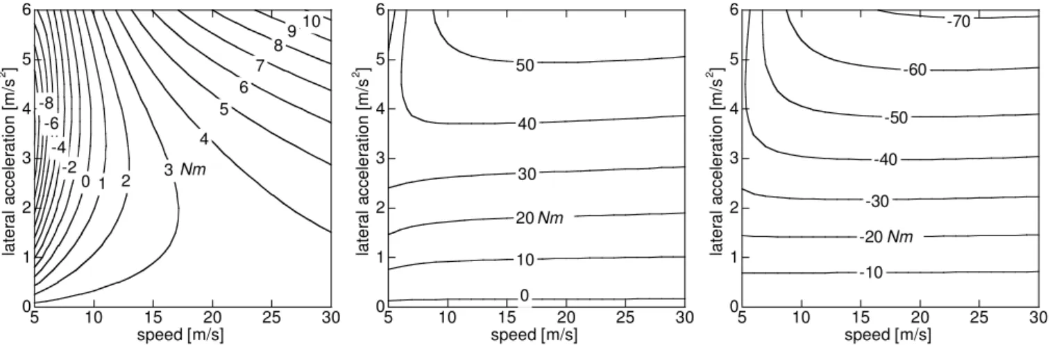
The steering torque components are now analyzed. The main contributes to the whole torque are those related to the tyre normal load and to the tyre lateral force. In particular the torque related to the normal load (Figure 6) is always misaligning, whereas the torque related to the lateral force (Figure 7) is always aligning. For example, at 20 m/s and 4 m/s2 the normal load generates a misaligning torque of +42.3 Nm, whereas the tyre lateral force generates an aligning torque of -51.8 Nm, i.e. these two components almost balance each other to give an aligning torque of -9.5 Nm (which will be balanced by the rider’s reaction +9.5 Nm). Moreover, Figure 6 and Figure 7 show that these torques depend only on lateral acceleration for speeds higher than 15-20 m/s. It is interesting to note that these contributes change significantly at low speeds (lower than 10 m/s) and important lateral accelerations (higher than 4 m/s2). This effect is mainly due to the variation of the forces arm at low speeds, as shown in Figure 10 which depicts the normal trail (i.e. the distance between the road-tyre contact point and the steering axis). This effect is even more pronounced has the roll angle (i.e. the lateral acceleration) increases, see [1].
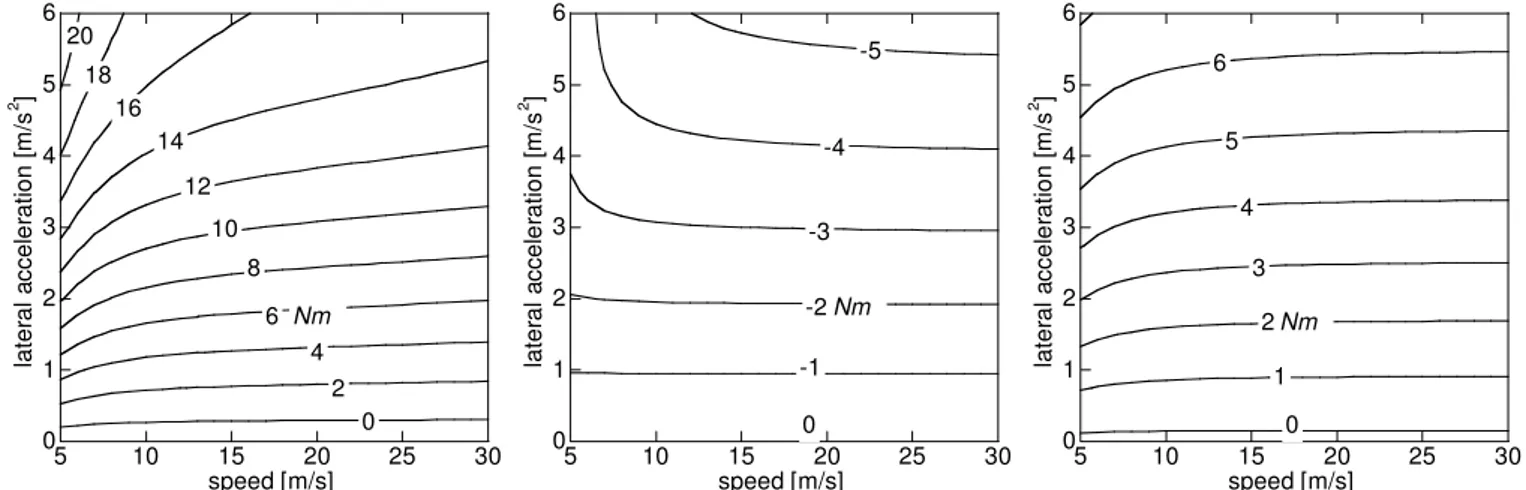
As a consequence of the tyre carcass hysteresis a rolling torque opposes the wheel rotation and a friction force arises. The longitudinal friction force on the front tyre leads to a small misaligning contribute to the steering torque, see Figure 8. Its presence is due to the fact that the tyre carcass is
not a thin disk, and therefore the longitudinal force has a not-null arm when the vehicle is leaned because of the migration of the contact point on the tyre carcass. The tyre rolling torque also gives a contribute to the steering torque, see Figure 9: it is always aligning and is related to the fact that when the vehicle is leaned, the rolling torque projection on the steering axis is no more null. It is interesting to observe that, given the lateral acceleration, these contributes first decrease in magnitude, then increase in magnitude for speeds higher than 10-15 m/s. Moreover this effect is more visible as the lateral acceleration increases. Once again, at low speed torques are influenced by the large variation in normal trail and steering angle. Another important contribute is the one related to the tyre yaw torque. This torque arises because the road-tyre contact does not take place in a point but on a patch, see [1],[20]. This contribute to the steering torque is always misaligning and significant, see Figure 11. Figure 12 depicts the gyroscopic contribute to the steering torque. The gyroscopic effect arises because the front wheel is both rolling about its spin axis and yawing as a consequence of the cornering manoeuvre. Its component is always aligning; again significant changes are present at low speeds and important lateral acceleration where the steering angle changes a lot and thus the projection of the gyroscopic torque on the steering axis changes too. Finally, minor components are those related to the front frame weight (misaligning), see Figure 13, and to the front frame centrifugal effect (aligning), see Figure 14.
0 1 2 3 4 5 6
5 10 15 20 25 30
later
al a
c
c
el
e
rati
o
n
[m
/s
2 ]
speed [m/s] 3 0
4 5
6 7
89 10
1 2 -2 -4 -6 -8
Nm
Figure 5. Rider steering torque.
0 1 2 3 4 5 6
5 10 15 20 25 30
later
al a
c
c
el
e
rati
o
n
[m
/s
2 ]
speed [m/s] 30
0 40 50
10 20Nm
Figure 6. Tyre normal load N component.
0 1 2 3 4 5 6
5 10 15 20 25 30
later
al a
c
c
el
e
rati
o
n
[m
/s
2 ]
speed [m/s] -10
Nm
-20 -30
-40 -50
-60 -70
Figure 7. Tyre lateral force F component.
0 1 2 3 4 5 6
5 10 15 20 25 30
later
a
l a
c
c
e
ler
a
ti
on
[m
/s
2 ]
speed [m/s] 0.5
0
Nm
1 1.5 2.5
2 3
Figure 8. Tyre longitudinal force S component. 0 1 2 3 4 5 6
5 10 15 20 25 30
later
a
l a
c
c
e
le
ra
ti
on
[m/s
2 ]
speed [m/s] 0
-1 -2
-4 -6
Nm
-3 -5
-7 -8
Figure 9. Tyre rolling torque Tycomponent. 0 1 2 3 4 5 6
5 10 15 20 25 30
later
a
l a
c
c
e
le
ra
ti
on
[m/s
2 ]
speed [m/s] 110
mm
112
114 100
60
80
V. EFFECTOFLONGITUDINALACCELERATIONS When braking or accelerating the steering torque necessary to negotiate the curve changes because the inertial forces and torques lead to a new equilibrium configuration. In this section the numerical model is used to compute the equilibrium steering torque while cornering at different speeds (5-30 m/s) and lateral accelerations (0-6 m/s2) with two values of longitudinal accelerations, ± 6m/s2.
First the braking condition is addressed. Since the same deceleration may be obtained with different braking strategies, e.g. only front braking, only rear braking, 50% front and 50% rear, etc., it has been chosen to divide the braking effort between front and rear axle in order to have the same longitudinal slip on both tyres. This approach is considered the best braking strategy [24]. Figure 15 depicts the difference between the equilibrium steering torque in braking condition and the equilibrium steering torque without longitudinal acceleration. It is worth noting that the differences are significant and more pronounced as the lateral acceleration increases. A deeper investigation reveals that the components of the steering torque due to the gyroscopic torques, centrifugal forces and weight forces do not change when braking, since their magnitudes do not depend on longitudinal acceleration and their arms are almost unchanged. On the contrary, the five torque components related to road-tyre interaction change significantly. Indeed
when braking on curve there is both a normal load transfer and a lateral force transfer from the rear axle to the front axle. While the normal load transfer is obvious, the lateral force transfer is not. In order to make things clearer, the expressions of the normal loads Nr,f and lateral forces Fr,f are reported below for the simple case of a vehicle with no aerodynamic force and null steer angle
cos arctan
cos arctan
y
r x r r
y
f x f f
y
y
a w b h
N a M F N
w w g
a b h
N a M F N
w w g
a g g a g g − = + = = − = ⎛ ⎞ ⎛ ⎞ ⎜ ⎟ ⎜ ⎟ ⎝ ⎝ ⎠⎠ ⎛ ⎞ ⎛ ⎞ ⎜ ⎟ ⎜ ⎟ ⎝ ⎝ ⎠⎠
where M is the mass, w is the wheelbase, b and h are the coordinates of the c.g., ax is the longitudinal acceleration, ay
is the lateral acceleration, subscript r is used for the rear tyre while subscript f is used for the front tyre.
The analysis of the torque components related to the road-tyre interaction reveals that because of the increased front normal load and front lateral force, both aligning and misaligning components increase their magnitude. Anyway the main effect is the misaligning torque due to the front braking force (Figure 16), whereas the increment of the aligning effect of tyre lateral force is almost balanced by the increase of the misaligning effect of tyre normal force, and the increment of the aligning effect of tyre rolling resistance torque is almost balanced by the increase of the misaligning effect of tyre yaw torque. From the dynamic point of view the
0 1 2 3 4 5 6
5 10 15 20 25 30
later a l a c c e le ra ti o n [ m /s 2 ] speed [m/s] 0 2 4 6 8 Nm 10 12 14 16 18 20
Figure 11. Tyre yaw torque Tz component.
0 1 2 3 4 5 6
5 10 15 20 25 30
later a l a c c e le ra ti o n [ m /s 2 ] speed [m/s] 0 -2 -4 Nm -1 -5 -3
Figure 12. Gyroscopic torque Tω component. 0 1 2 3 4 5 6
5 10 15 20 25 30
later a l a c c e le ra ti o n [ m /s 2 ] speed [m/s] 3 0 4 5 6 1 2Nm
Figure 13. Weight force W component.
0 1 2 3 4 5 6
5 10 15 20 25 30
later a l a c c e le ra ti on [m/s 2 ] speed [m/s] 0 -3 -4 Nm -1 -2 -5
Figure 14. Centrifugal force C component. 0 1 2 3 4 5 6
5 10 15 20 25 30
later a l a c c e le ra ti on [m/s 2 ] speed [m/s] 0 -5 -10 -15 Nm -20 -25
Figure 15. Effect of a deceleration of 6 m/s2
on rider steering torque.
0 1 2 3 4 5 6
5 10 15 20 25 30
la te ra l a c ce le ra ti on [ m /s 2 ] speed [m/s] 0 10 5 Nm 15 20 25 30 35 40
fact that the steering torque is significantly affected by the braking effort means that there is a strong coupling between in-plane and out of plane dynamics when braking while cornering. Please note that this coupling is strongly correlated to the shape of the front tyre carcass and increases with the tyre size. The analysis also explains why when braking on curve the vehicle is likely to naturally reduce the roll angle. Let’s suppose a rider is running on a curve with constant speed and constant lateral acceleration, i.e. roll angle. At some point he brakes using the front brake, as a consequence the new equilibrium steering torque is much more misaligning. If the rider does not promptly adapt his handlebar torque, the vehicle is no more in equilibrium and the steer angle increases due to the excess of misaligning torque. This causes an increment of the sideslip angle and of the lateral force that tends to straighten the motorcycle [6].
When accelerating the steering torque map does not change significantly as it does in braking condition. Indeed, the front tyre longitudinal force is not subjected to significant variation as while braking. As well as the other components is concerned, they do not change the steering torque since the situation is very similar to the braking one, with all load transfers reversed. From the dynamic point of view the fact that the steering torque is not significantly affected when accelerating means that there is a weak coupling between in-plane and out of plane dynamics when accelerating while cornering. In other words when a rider accelerates while cornering he does not feel the vehicle changing its roll, or at least not as much as he feels when braking.
VI. CONCLUSION
A detailed motorcycle multibody code has been used to investigate the steering torque while cornering. The multibody model has been successfully validated against experimental tests with three different motorcycles, then the decomposition of the steering torque has been addressed. The components are related to road-tyre contact forces and torques, gravity, centrifugal forces and gyroscopic torques. The effect of longitudinal acceleration on the components of steering torque has been investigated, finding significant changes while braking but minor effect when accelerating.
REFERENCES
[1] V. Cossalter, Motorcycle Dynamics, Lulu.com, 2006, ISBN: 978-1-4303-0861-4.
[2] D. H. Weir, J. W. Zellner, “Development of handling test procedures for motorcycles”, SAE paper 780313, 1978.
[3] R. S. Rice, “Rider skill influences on motorcycle manoeuvring”, SAE paper 780312, 1978.
[4] V. Cossalter, A. Doria, R. Lot. “Steady Turning of Two-Wheeled Vehicles”. Vehicle System Dynamics, 31, pp. 157–181, 1999. [5] R.S. Sharp, “Stability, Control and Steering Responses of
motorcycles”, Vehicle System Dynamics, Vol. 35, 4-5, 291-318, 2001. [6] V. Cossalter, R. Lot, M. Peretto, “Motorcycles Steady Turning”,
Journal of Automobile Engineering, Vol. 221 Part D, pp. 1343-1356, 2007.
[7] P.T.J. Spierings, “The effect of lateral front fork flexibility on the vibration modes of straight-running single-track vehicles”, Vehicle System Dynamics, 10, 21-35, 1981.
[8] C. Koenen, H.B. Pacejka, “Influence of Frame Elasticity, Simple Rider Body Dynamics and Tyre Moments on Free Vibrations of Motorcycles in Curves”, in Proc. of the IAVSD Symposium, 1982.
[9] T. Hikichi, K. Takaci, “Dynamic Characteristics of a Motorcycle with a Single-Side Supported Swing Arm”, SAE 905214, 721-731, 1990. [10] Y. Marumo, T. Katayama, “Effects of Structural Flexibility on Weave
Mode of Motorcycle”., in Proc of the 6th International Symposium on Advanced Vehicle Control, Hiroshima, Japan, 2002.
[11] V. Cossalter, R. Lot, M. Massaro, “The influence of Frame Compliance and Rider Mobility on the Scooter Stability”, Vehicle System Dynamics, 45, 315-326, 2007.
[12] T. Katayama, A. Aoki, T. Nishimi, T. Okayama, “Measurement of Structural Properties of Riders”, in Proc. of the 4th International Pacific Conference on Automotive Engineering, Melbourne, Australia, 1987. [13] T. Nishimi, A. Aoki, T. Katayama, “Analysis of Straight Running
Stability of Motorcycles”, in Proc. of the 10th International Technical Conference on Experimental Safety Vehicles, Oxford, England, 1985. [14] Y. Marumo, T. Katayama, “Effect of Motorcycle Tandem Riding on
Weave Mode Stability”, Thesis collection of the Journal of Automotive Technology Association, v 36, n 6, 2005.
[15] R.S. Sharp, D.J.N. Limebeer, “On steering oscillations of motorcycles”, in Proc. of IMechE., Part C, Journal of Mechanical Engineering Science, Vol.18, 2004, 1449-1456.
[16] V. Cossalter, A. Doria, R. Lot, M. Massaro, “The effect of rider's steering impedance on motorcycle stability: identification and analysis”, Meccanica, submitted for publication.
[17] V. Cossalter, R. Lot, “A Motorcycle Multi-Body Model for Real Time Simulations Based on the Natural Coordinates Approach”, Vehicle System Dynamics, vol. 37, n. 6 pp. 423-447, 2002.
[18] V. Cossalter, R. Lot, M. Massaro, “The chatter of racing motorcycle”, Vehicle System Dynamics, 46, pp. 339-353, 2008.
[19] R. Lot, M. Da Lio, “A Symbolic Approach for Automatic Generation of the Equations of Motion of Multibody Systems”, Multibody System Dynamics, 12, 147-172, 2004.
[20] H.B. Pacejka, Tyre and vehicle dynamics, SAE International, 2005, ISBN: 978-0-7680-1702-1.
[21] R. Lot, “A Motorcycle Tyre Model for Dynamic Simulations: Theoretical and Experimental Aspects”, Meccanica, Vol 39, pp 204-218 ISSN 0025-6455, 2004.
[22] V. Cossalter, A. Doria, R. Lot, N. Ruffo, M. Salvador, “Dynamic Properties of Motorcycle and Scooter Tires: measurement and comparison”, Vehicle System Dynamics: International Journal of Vehicle Mechanics and Mobility , Vol. 39, No. 5, pp. 329-352, 2003. [23] M. Da Lio, A. Doria, R. Lot, “A Spatial Mechanism for the
Measurement of the Inertia Tensor: Theory and Experimental Results”, ASME, Journal of Dynamic Systems, Measurement, and Control, Vol. 121, pp.111-116, 1999.