U
niversidade de S˜
ao Paulo
I
nstituto de F´ısica
Observational Constraints on Models
with an Interaction between Dark
Energy and Dark Matter
A
ndr´
e Alencar da Costa
Advisor: Prof. Dr. Elcio Abdalla
Thesis presented to the Institute of Physics
of the University of S˜ao Paulo in partial
ful-fillment of the requirements for the degree of
Doctor in Science
Examining Commission:
Prof. Dr. Elcio Abdalla (IF-USP)
Prof. Dr. Luis Raul Weber Abramo (IF-USP)
Prof. Dr. Marcos Vinicius Borges Teixeira Lima (IF-USP)
Prof. Dr. Ioav Waga (IF-UFRJ)
Prof. Dr. Lu´ıs Carlos Bassalo Crispino (FACFIS-UFPA)
S˜ao Paulo
- - -
FICHA CATALOGRÁFICA
Preparada pelo Serviço de Biblioteca e Informação
do Instituto de Física da Universidade de São Paulo
Costa, André Alencar da
Observational constraints on models with an interaction between dark energy and dark matter / Vínculos observacionais em modelos com interação entre energia escura e matéria escura. São Paulo, 2014.
Tese (Doutorado) – Universidade de São Paulo. Instituto de Física. Depto. de Física Matemática
Orientador: Prof. Dr. Elcio Abdalla
Área de Concentração: Física
Unitermos: 1. Cosmologia; 2. Matéria escura; 3. Energia escura.
U
niversidade de S˜
ao Paulo
I
nstituto de F´ısica
V´ınculos Observacionais em Modelos
com Intera¸
c˜
ao entre Energia Escura
e Mat´
eria Escura
A
ndr´
e Alencar da Costa
Orientador: Prof. Dr. Elcio Abdalla
Tese de doutorado apresentada ao Instituto
de F´ısica para a obten¸c˜ao do t´ıtulo de Doutor
em Ciˆencias
Banca Examinadora:
Prof. Dr. Elcio Abdalla (IF-USP)
Prof. Dr. Luis Raul Weber Abramo (IF-USP)
Prof. Dr. Marcos Vinicius Borges Teixeira Lima (IF-USP)
Prof. Dr. Ioav Waga (IF-UFRJ)
Prof. Dr. Lu´ıs Carlos Bassalo Crispino (FACFIS-UFPA)
S˜ao Paulo
Acknowledgments
First of all I would like to thank my advisor Elcio Abdalla for his guidance and patience. I
also acknowledge him for the incentive to scientific independence and for the high quality
research environment he provided me.
Many thanks to the several collaborators during the years of the doctorate, especially
professor Bin Wang for helpful discussions about phenomenological models on interacting
dark energy, and the colleagues Elisa Ferreira, Leila Graef, Lucas Olivari, Riis Rhavia and
Xiao-Dong Xu.
I am also very grateful to the colleagues of the department of mathematical physics
for the friendship, especially my office mates Eduardo Matsushita, Ricardo Pereira, Lucas
Secco, Arthur Loureiro and Carolina Queiroz.
I could not forget the couple Jacinto and Bernadete for their hospitality and generosity,
opening the doors of their home to me and my wife for the first month we arrived in S˜ao
Paulo. I also thank their children and grandchildren for all the moments we passed
together.
During these years in S˜ao Paulo I was benefited by the friendship of many people,
especially I would like to thank the people of the Presbyterian Church in Jardim Bonfiglioli
who have been a second family to me, my wife and now my daughter.
Certainly I would not have arrived here without the encouragement and support of
my family and friends. I am especially grateful for my wife Lidiane, for her love, standing
on my side all these years even with the cost of being apart from her family, and my
daughter Ana Beatriz, who made these last months full of happiness and pleasure.
I gratefully acknowledge the partial financial support from CAPES, Coordena¸c˜ao de
Aperfei¸coamento de Pessoal de N´ıvel Superior, and the financial support from CNPq,
Conselho Nacional de Desenvolvimento Cient´ıfico e Tecnol´ogico - Brasil. This work would
This work has made use of the computing facilities of the Laboratory of
Astroinfor-matics (IAG/USP, NAT/Unicsul), whose purchase was made possible by the Brazilian
Abstract
In this thesis we go beyond the standard cosmological ΛCDM model and study the
ef-fect of an interaction between dark matter and dark energy. Although the ΛCDM model
provides good agreement with observations, it faces severe challenges from a theoretical
point of view. In order to solve such problems, we first consider an alternative model
where both dark matter and dark energy are described by fluids with a phenomenological
interaction given by a combination of their energy densities. In addition to this model, we
propose a more realistic one based on a Lagrangian density with a Yukawa-type
interac-tion. To constrain the cosmological parameters we use recent cosmological data, the CMB
measurements made by the Planck satellite, as well as BAO, SNIa,H0 and Lookback time
measurements.
Resumo
Nesta tese vamos al´em do modelo cosmol´ogico padr˜ao, o ΛCDM, e estudamos o efeito
de uma intera¸c˜ao entre a mat´eria e a energia escuras. Embora o modelo ΛCDM esteja
de acordo com as observa¸c˜oes, ele sofre s´erios problemas te´oricos. Com o objetivo de
resolver tais problemas, n´os primeiro consideramos um modelo alternativo, onde ambas,
a mat´eria e a energia escuras, s˜ao descritas por fluidos com uma intera¸c˜ao fenomenol´ogica
dada como uma combina¸c˜ao das densidades de energia. Al´em desse modelo, propomos
um modelo mais realista baseado em uma densidade Lagrangiana com uma intera¸c˜ao tipo
Yukawa. Para vincular os parˆametros cosmol´ogicos usamos dados cosmol´ogicos recentes
como as medidas da CMB feitas pelo sat´elite Planck, bem como medidas de BAO, SNIa,
H0 e Lookback time.
Contents
Introduction 1
1 Introduction to Cosmology: The Need of Dark Matter and Dark Energy 3
1.1 Homogeneous and Isotropic Universe . . . 3
1.2 Cosmic Distances . . . 7
1.3 Components of the Universe . . . 10
1.3.1 The Standard Model of Particle Physics . . . 10
1.3.2 Photons . . . 12
1.3.3 Baryons . . . 14
1.3.4 Neutrinos . . . 15
1.3.5 Dark Matter . . . 17
1.3.6 Dark Energy . . . 18
2 Cosmological Perturbations 21 2.1 Perturbed Metric . . . 21
2.2 Einstein Equations . . . 24
2.3 Boltzmann Equation . . . 25
2.3.1 Photons . . . 26
2.3.2 Baryons . . . 32
2.3.3 Neutrinos . . . 36
2.3.4 Dark Matter . . . 37
2.3.5 Energy-Momentum Tensor . . . 37
2.4 Initial Conditions . . . 38
2.5 Inhomogeneities: Matter Power Spectrum . . . 41
3 Interacting Dark Energy 45
3.1 Phenomenological Model . . . 45
3.2 Lagrangian Model . . . 55
3.2.1 The Tetrad Formalism . . . 56
3.2.2 Yukawa-Type Interaction . . . 58
4 Analysis 66 4.1 Methods for Data Analysis . . . 66
4.2 Data . . . 69
4.2.1 CMB Measurements . . . 69
4.2.2 BAO Measurements . . . 70
4.2.3 SNIa Measurements . . . 71
4.2.4 H0 Measurements . . . 72
4.2.5 Lookback Time Measurements . . . 72
4.3 Results . . . 73
4.3.1 Phenomenological Model . . . 73
4.3.2 Lagrangian Model . . . 88
Conclusions 94
A Camb Code: Phenomenological Model 96
B Camb Code: Lagrangian Model 101
C CosmoMC Code: Lookback Time 115
Introduction
The large amount of precise astronomical data released in the past few years provided
opportunities to answer questions in cosmology and astrophysics. Such a precision allows
us to test cosmological models and determine cosmological parameters with high accuracy.
The simplest cosmological model one can build that reasonably explains the current
data is the ΛCDM model. This model consists in a cosmological constant Λ to account
for the observed acceleration of the Universe, plus cold dark matter (CDM) necessary to
produce the gravitational potential wells inferred on galactic to cosmological scales.
However, theoretically the ΛCDM model itself faces challenges, the cosmological
con-stant problem[1] and the coincidence problem[2]. The first one refers to the small observed
value of the cosmological constant, incompatible with the vacuum energy description in
field theory. The second one refers to the fact that we have no natural explanation for
why the energy densities of dark matter and vacuum energy are of the same order today.
These problems open the avenue for alternative models of dark energy to substitute the
cosmological constant description.
One way to alleviate the coincidence problem, which embarrasses the standard ΛCDM
cosmology, is to consider an interaction between dark energy and dark matter.
Consider-ing that dark energy and dark matter contribute with significant fractions of the contents
of the Universe, it is natural, in the framework of field theory, to consider an interaction
between them. The interaction between dark energy and dark matter will affect
signifi-cantly the expansion history of the Universe and the evolution of density perturbations,
changing their growth. The possibility of the interaction between dark sectors has been
widely discussed in the literature [3–36]. Determining the existence of dark matter and
dark energy interactions is an observational endeavor that could provide an interesting
insight into the nature of the dark sectors.
Since the physical properties of dark matter and dark energy at the present moment
are unknown, we cannot derive the precise form of the interaction from first principles. For
simplicity, most considerations of the interaction in the literature are from phenomenology.
Attempts to describe the interaction from field theory have been proposed in [37–39]. One
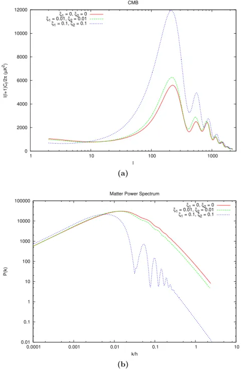
possibility is a phenomenological model of the interaction, Q, between dark matter and
dark energy, which is in a linear combination of energy densities of the dark sectors
Q = 3H(ξ1ρc +ξ2ρd) [13, 29, 40]. In this interaction, H is the Hubble parameter, ξ1
and ξ2 are dimensionless parameters, assumed to be time independent, for simplicity,
and ρc and ρd are the energy densities of dark matter and dark energy, respectively.
Such a model was widely studied in [13, 18, 34, 41–44]. It was disclosed by the late
integrated Sachs-Wolf (ISW) effect [25, 27] that the interaction between dark matter
and dark energy influences the cosmic microwave background (CMB) at low multipoles
and at high multipoles through gravitational lensing [44, 45]. With the WMAP data
[25, 27] together with galaxy cluster observations [34, 35] and also recent kinetic
Sunyaev-Zel’dovich effect observations [46], it was found that this phenomenological interaction
between dark energy and dark matter is viable and the coupling constant is positive,
indicating that there is energy flow from dark energy to dark matter, which is required to
alleviate the coincidence problem and to satisfy the second law of thermodynamics [16].
It is of great interest to build alternative models of the Universe and employ the
latest high-precision data to further constrain them. This is the main motivation of the
present work. We will combine the CMB data from Planck [47–49] with other cosmological
probes such as the baryonic acoustic oscillations (BAO) [50–52], supernovas [53], the latest
constraint on the Hubble constant [54] and lookback time [55, 56]. We want to see how
these different probes will influence the cosmological parameters and put tight constraints
on the interaction between dark sectors.
This thesis is organized as follows: in the first chapter we introduce some fundamental
aspects of cosmology and present the contents of the Universe. Chapter two goes beyond
the homogeneous and isotropic universe and describe the linear perturbations. Our models
of interactions between dark energy and dark matter are presented in chapter three. The
data analysis and our fitting results appear in chapter four. Finally, we conclude and
Chapter 1
Introduction to Cosmology: The
Need of Dark Matter and Dark
Energy
Cosmology is the study of the Universe as a whole. Despite the great complexity of this
system, if we are interested in its dynamics on large scales, it is possible to construct
a relatively simple model to describe it. On large scales, the interactions between the
constituents of the Universe are governed by the laws of gravitation which, nowadays, are
best explained by the theory of general relativity published by Einstein in 1915 [57].
1.1
Homogeneous and Isotropic Universe
General relativity establishes that the geometry of the spacetime is determined by the
energy content of the Universe and this geometry governs the motion of free particles. In
general, the geometry of the spacetime is described by the line element
ds2 =gµνdxµdxν, (1.1)
wheregµν are the components of the metric tensor. The indicesµ, ν are defined such that
x0represents the time coordinate andxi, withi= 1,2,3, represent the spatial coordinates. We are using the Einstein’s convention where repeated indices are summed.
To determine the form of the line element of a given cosmological model we use the
underlying symmetries. The simplest cosmological model can be built assuming that the
constituents of the Universe present the properties of statistical homogeneity and isotropy,
known as the cosmological principle. In fact, observations of the cosmic microwave back-ground have shown isotropy of one part in 100.000 [58]. Also, evidences of galaxy surveys
suggest that the Universe is homogeneous on large scales [59].
Using the cosmological principle, the metric of the spacetime must be the
Friedmann-Lemaitre-Robertson-Walker (FLRW) metric [57], which is given by
ds2 =−dt2+a(t)2
dr2
1−Kr2 +r
2 dθ2+ sin2θdφ2
. (1.2)
Herea(t) is a scale factor accounting for the expansion or contraction of the Universe and
K is a constant that establishes the geometry of the spatial section. If K >0 the spatial
section is closed, while for K = 0 it is flat and K < 0 means that the spatial section is
open. Throughout this work we are using natural units such that ¯h=c=kB = 1.
The motions of free particles follow the geodesic equations
d2xµ
dλ2 + Γ
µ αβ
dxα
dλ dxβ
dλ = 0, (1.3)
where λ is a monotonically increasing parameter that parameterizes the particle’s path
and Γµαβ are the Christoffel symbols. The Christoffel symbols are related to the metric
tensor by the expression
Γµαβ = g µν
2
∂gαν
∂xβ +
∂gβν
∂xα −
∂gαβ
∂xν
, (1.4)
wheregµν is the inverse of the metric tensor such thatgµαg
αν =δµν withδνµ, the Kronecker
delta, defined as zero unless µ=ν in which case it is equal to one.
To obtain a(t) and K we need the dynamical equations governing the Universe. In
the context of general relativity it is determined by the Einstein equations [60]
Rµν− 1
2gµνR = 8πGTµν, (1.5)
where Rµν is the Ricci tensor, which can be written in terms of the Christoffel symbol as
Rµν =
∂Γα µν
∂xα −
∂Γα µα
∂xν + Γ α
1.1. HOMOGENEOUS AND ISOTROPIC UNIVERSE 5
R=gµνR
µνis the Ricci scalar, or curvature scalar,Gis the Newton gravitational constant
andTµν is the energy-momentum tensor of the content in the Universe. All the quantities
in the left hand side of (1.5) are geometrical quantities, while the right hand side presents
the energy content. Thus, the Einstein equations relate the geometry of the Universe to
the energy content.
On large scales the constituents of the Universe can be treated as a fluid. The most
general energy-momentum tensor for a fluid component “A”, TA
µν, is given by
TµνA = (ρA+PA)uAµuAν +gµνPA+πAµν+qAµuνA+qνAuAµ, (1.7)
where ρA is the energy density, PA is the pressure, uA
µ is the four-velocity vector, πµνA is
the anisotropic stress andqA
µ is the heat flux vector relative touAµ, all these quantities with
respect to the A-fluid. The total energy-momentum tensor is Tµν = PATµνA. However,
if the fluid has at each point a velocity~v, such that an observer with this velocity sees
the fluid around him as isotropic, this is known as aperfect fluid [57] and in this case the anisotropic stress and the heat flux are null.
Using the FLRW metric (1.2) and the energy-momentum tensor (1.7) for all
compo-nents with the assumption of a perfect fluid, the Einstein equations (1.5) result in two
independent equations. The time-time component gives the Friedmann equation
H2(t) = 8πG 3 ρ(t)−
K
a2(t) (1.8)
and the space-space components result in
˙
H(t) =−4πG[ρ(t) +P(t)] + K
a2(t), (1.9)
where H(t)≡ a˙(t)/a(t) is called Hubble parameter, ρ, P denote the total energy density and pressure and a dot means differentiation with respect to the cosmic time t.
We can define a critical densityρcrit by
ρcrit ≡
3H2(t)
8πG , (1.10)
it. Constructing the density parameter Ω as
Ω = X
A
ΩA≡ X
A
ρA
ρcrit
, (1.11)
the Friedmann equation (1.8) can be rewritten as
Ω−1 = K
H2(t)a2(t). (1.12)
From this equation we can see that the curvature of the spacial section K is determined
by the energy content of the Universe. In fact,
ρ < ρcrit ⇒Ω<1⇒K <0,
ρ=ρcrit ⇒Ω = 1⇒K = 0,
ρ > ρcrit ⇒Ω>1⇒K >0.
(1.13)
To solve the Friedmann equation (1.8) and find how the scale factor a(t) evolves with
time, we have to know what is the dependence ofρwith time, or equivalently with the scale
factor. Combining (1.8) and (1.9), or using the conservation of the energy-momentum
tensor, results
˙
ρ+ 3H(ρ+P) = 0. (1.14)
As (1.14) can be obtained from (1.8) and (1.9), it means that only two of equations (1.8),
(1.9) and (1.14) are independent. Equation (1.14) is valid for the total energy density, but
if the individual components are independent, they will obey similar equations. Thus, if
we know what are the components of the Universe and the equation of state they satisfy,
we can solve Eq. (1.14) for each individual component and find their dependence with
the scale factor. Knowing this, we can solve the Friedman equation (1.8).
There is another relation that can be obtained from equations (1.8) and (1.9).
Elimi-nating K/a2 from those equations, we obtain
¨
a a =−
4πG
3 (ρ+ 3P). (1.15)
This equation tells us that an accelerated expansion only occurs if ρ+ 3P < 0. As the
accel-1.2. COSMIC DISTANCES 7
erated expansion, the Universe must contain some component with a negative pressure.
Considering a fluid with a linear barotropic equation of state1, P = ωρ, the accelerated
expansion can occur if w <−1/3.
1.2
Cosmic Distances
In the previous section we established a theoretical model for a homogeneous and isotropic
universe. Solving the system of equations (1.8) and (1.14) allows us to determine the
evolution of the scale factora(t) and consequently the history of the Universe. However,
to solve that system of equations we need to determine the values of some parameters
as K, the initial value of H(t), the initial energy densities of all the constituents of the
Universe and their equation of state, usually assumed to be of the form ω = P/ρ. To
describe the real Universe these parameters must be in agreement with observations,
which means we need observables that allow us to compare theory with observations.
A fundamental step to compare theory with observations is the measurement of
dis-tances on cosmological scales. These measurements enable us to relate physical
observ-ables with the parameters in our model such that we can constrain it and make predictions.
Actually, there are several ways to define distances in cosmology as we show below.
From the FLRW line element (1.2), a light ray traveling along the radial direction
satisfies the geodesic equation
ds2 =−dt2+a2(t)dχ2 = 0, (1.16)
where we defined dχ ≡ dr/(1−Kr2)1/2. Therefore, considering that a light ray have
traveled from the timet= 0, we can find the total comoving distance that it could travel
until the timet as
η≡
Z t
0 dt′
a(t′). (1.17)
This distance establishes a limit beyond which no information can further propagate
in the comoving frame. Thus, η can be thought as a comoving horizon. Because η
is monotonically increasing, it can also be defined as a time variable, which is called
conformal time. Using equation (1.16), we can obtain the comoving distance from a
distant object at scale factor a to us:
χ(a) = Z t0
t(a) dt′
a(t′) =
Z a0
a
da′
a′2H(a′), (1.18)
where the subscript “0” represents quantities at the present time.
The comoving coordinates are constant over the expansion history of the Universe.
Thus, using Eq. (1.18), a light ray emitted at time t+δt and observed at time t0+δt0
satisfies
Z t0
t
dt′
a(t′) =
Z t0+δt0
t+δt
dt′
a(t′). (1.19)
Manipulating the limits of integration, we can write
Z t+δt t
dt′
a(t′) =
Z t0+δt0
t0
dt′
a(t′). (1.20)
At first order in δt we have
δt a(t) =
δt0
a(t0). (1.21)
Ifδtis the period of emission of the light ray and δt0 the period of detection, as the wave
frequency ν is the inverse of the period and the wave length is defined as λ = c/ν, we
obtain
1 +z ≡ νemit νobs
= λobs
λemit = a0
a . (1.22)
This expression defines a cosmological Doppler effect associated with the expansion or
contraction of the Universe. To account with this effect we defined the redshift z. The
above equation allows us to relate the redshift of a distant object to the scale factor when
the light ray was emitted.
Basically, there are two ways of inferring distances in astronomy: using a standard ruleror astandard candle. With the knowledge of trigonometry astronomers have inferred lengths for a long time. Measuring the angle θ subtended by an object of known physical
size l (a standard ruler), the distance to that object is
dA=
l
2 tan(θ
2) ≈ l
θ, (1.23)
1.2. COSMIC DISTANCES 9
we can see that the physical lengthl of an object described by an angle θ is given by
l=a(t)rθ. (1.24)
Therefore, comparing Eqs. (1.23) and (1.24), we observe that the angular diameter dis-tanceis
dA=a(t)r=a(t)
1
H0√Ωk0 sinh(H0 √
Ωk0χ) Ωk>0,
χ Ωk= 0,
1
H0√−Ωk0 sin(H0 √
−Ωk0χ) Ωk<0,
(1.25)
where we used the definitions of χand Ωk≡ −K/H2(t)a2(t), and we are using a normal-ization such that a0 = 1.
Another important technique to determine distances is to find an object of known
intrinsic brightness, a standard candle, such that any difference between the apparent brightness of two of these objects is a result of their different distances from us. Given an
object of known luminosityL, the observed flux F a distance dL from the source is
F = L 4πd2
L
. (1.26)
On an expanding universe we can write a similar equation considering a comoving grid as
F = L(χ)
4πr2(χ), (1.27)
whereL(χ) is the luminosity of the source through a comoving spherical shell with radius
r(χ). Assuming that the photons are emitted with the same energy, the luminosityL(χ)
is the energy multiplied by the number of photons crossing the shell per unit time. As
the Universe expands, the number of photons passing through the spherical shell per unit
time becomes smaller by a factor of a. On the other hand, Eq. (1.22) tells us that the
wave lengths of the photons are stretched by a factor of 1/a. Thus, as the energies of
the photons are inversely proportional to the wave length, they will decrease accordingly.
Therefore, the energy per unit time on the spherical shell at r(χ) will be a factor of a2
smaller than the luminosity at the source
F = La
2
If we define theluminosity distance dL as
dL≡
r(χ)
a =
1
a(t)
1
H0
√
Ωk0 sinh(H0 √
Ωk0χ) Ωk >0,
χ Ωk = 0,
1
H0
√
−Ωk0 sin(H0 √
−Ωk0χ) Ωk <0,
(1.29)
we can keep the form of the flux given by Eq. (1.26). Comparing Eq. (1.25) with Eq.
(1.29) we observe that
dA =a2(t)dL=
dL
(1 +z)2, (1.30)
which is valid in general since the flux is conserved [61].
From equations (1.18), (1.25) and (1.29) we see that in the limit z ≪ 1 all distances
recover the Euclidean distance in Minkowski spacetime.
1.3
Components of the Universe
To calculate the equation (1.14) we need to know what are the constituents of the Universe
and what are the equations of state they obey. Thus, we sketch below the standard model
of particle physics (SM) and describe some properties of the fundamental ingredients that
build the Universe.
1.3.1
The Standard Model of Particle Physics
The standard model of particle physics contains our present knowledge of the
fundamen-tal particles that compose all the material content in the Universe and the interactions
between them. The standard model consists in a gauge group
GSM ≡SU(3)c×SU(2)L×U(1)Y, (1.31)
whereU(N) is defined by its fundamental representation as the group of unitary matrices
N ×N and SU(N) is the group of special unitary matrices, i.e. unitary matrices N ×N
with determinant equal to 1. Thus, SU(3)c describes the internal symmetry for hadrons,
which are particles that can interact via the strong interaction because they have a color
charge c. This theory is described by Quantum Chromodynamics (QCD). On the other
1.3. COMPONENTS OF THE UNIVERSE 11
L, Y mean that the symmetries SU(2), U(1) correspond to left-handed doublets and
hypercharge, respectively.
The fundamental constituents of matter are fermions with spin 1/2 which are classified
as quarks or leptons. Quarks appear together forming hadrons such as: protons, neutrons,
pions, kaons, etc. They have color and interact strongly as explained by QCD. Leptons,
such as the electron and neutrino, have no color degree of freedom and cannot interact
via strong interaction. Besides this, neutrinos do not carry electric charge either, their
motion is influenced only by weak interaction.
In the standard model, interactions among quarks and leptons are mediated by gauge
bosons with spin 1. There are five types of gauge bosons: photons, which are responsible
for the electromagnetic interaction;W±andZ0, that mediate the weak interaction; finally,
the gluons in the strong interaction. Below is a sketch of the standard model:
1st Generation 2nd Generation 3rd Generation
Quarks uc dc L
, uc R, dcR,
cc sc L
, cc R, scR,
tc bc L
, tc
R, bcR, (1.32)
Leptons νe e− L
, e−
R, νµ µ− L
, µ−
R, ντ τ− L
, τ−
R, (1.33)
Gauge bosons photon γ,
weak bosons W±, Z0,
gluons g,
(1.34)
Higgs bosons H. (1.35)
We can see that quarks and leptons come in three generations. The corresponding
particles in each generation have the same quantum numbers except for its mass. The
first family is the less massive and the third is the most massive. The SU(3) triplets
are represented by the color index c and the SU(2) doublets are arranged in columns.
Also, the upper quarks have electric charge equal to 2/3 and the lower ones have charge
−1/3. On the other hand, neutrinos have no electric charge and their leptonic partners carry electric charge equal to−1. All of them have antiparticles with the same mass and
The last component of the standard model, the Higgs boson, is a scalar particle that
is responsible for the Higgs mechanism. In the gauge group (1.31) the particles cannot
be massive otherwise the symmetries are not preserved. Therefore, to obtain massive
particles as observed in Nature we have to break the symmetry group (1.31) at some time.
The Higgs mechanism accounts for that performing a spontaneous symmetry breaking
(SSB), where the Lagrangian remains symmetric under (1.31) while the physical vacuum
becomes non-invariant. In this way
SU(3)c×SU(2)L×U(1)Y →SU(3)c×U(1)Q, (1.36)
where Q denotes the electric charge generators.
The standard model of particle physics agrees pretty well with the observed particles
and the corresponding interactions. However, from a theoretical point of view, there are
some remarkable difficulties. Therefore, it is a consensus that a more fundamental theory
must exist coinciding with the standard model in the low-energy limit. It should also be
noted that the SM does not include gravitation.
As we said before, on large scales the behavior of the particles are governed by the
gravitational interaction. In fact the strong and weak interactions act only in the nuclear
range. On the other hand, the atoms that build the matter content are neutral and
have spin oriented randomly so that on large scale matter do not interact with each other
electromagnetically. Actually, these interactions are important in the early Universe when
it was hotter and denser, but can be neglected at more recent epochs.
1.3.2
Photons
For a dilute weakly-interacting gas withg∗ internal degrees of freedom, the number density
n, energy densityρ and pressureP are given by [60, 62]
n = g∗ (2π)3
Z
f(~x, ~p)d3p, (1.37)
ρ = g∗ (2π)3
Z
E(~p)f(~x, ~p)d3p, (1.38) P = g∗
(2π)3
Z
|~p|2
3E(~p)f(~x, ~p)d
1.3. COMPONENTS OF THE UNIVERSE 13
whereE2 =|~p|2+m2 and f(~x, ~p) is the phase space distribution function (or occupation
number) which counts the number of particles around position~xand momentum~pin phase
space. If some component is in kinetic equilibrium, i.e. is in equilibrium at temperature
T, the distribution function is
f(~x, ~p) = 1
e(E−µ)/T ±1, (1.40)
where µ is the chemical potential. Fermions obey Fermi-Dirac statistics which is
repre-sented by the above equation with the +1 sign and bosons obey Bose-Einstein statistics
that is given by the −1 sign.
Basically, all information of the outside space comes from photons. They have a
well known homogeneous and isotropic distribution at one part in 105. Presently, the
temperature amounts to T0 = 2.725(2) K as measured by the FIRAS instrument aboard
the COBE satellite [63]. Combining equations (1.38) and (1.39) for a relativistic particle
(kBT ≫m) we have that
P = 1
3ρ. (1.41)
Thus, photons obey a linear barotropic equation of state with ω = 1/3 and using (1.14)
we can see that their energy density evolves as ργ ∝a−4.
Photons can be described as a gas with a temperature given by the COBE satellite
and a chemical potential µ = 0, since they can be freely created or destroyed. In fact,
observationally, the limits on a chemical potential are|µ|/T <9×10⁻⁵ [64], thusµcan be
safely neglected. With these assumptions, and knowing that photons have two degenerate
states given by their polarizations, we obtain from (1.38)
ργ =
π2
15T
4. (1.42)
Sinceργ ∝a−4 this tells us that the temperature of the CMB must vary as T ∝a−1. With respect to the critical density today, the photon energy density is
ργ
ρcrit = π
2
15
2.725K a
4
1
8.098×10⁻¹¹h2eV4 =
2.47×10⁻⁵
h2a4 , (1.43)
whereh parameterizes the Hubble constant H0 = 100h kmsec−1M pc−1 and we used that
a normalization of a given by a0 = 1, we have Ωγ0 ≈5×10⁻⁵.
1.3.3
Baryons
Generally in cosmology, we call the protons, neutrons and electrons that together build
the atoms, as baryons. Although electrons are not baryons, but leptons, because their
masses are so small in comparison with that of the protons and neutrons, we can consider
that atoms are made of baryons. In this way, the baryons form all the known matter
content in the Universe.
Using equations (1.37), (1.38) and (1.39) for non-relativistic particles (m ≫ kBT),
both fermionic and bosonic components result in the same equations for the number
density, energy density and pressure
n = g∗
mT
2π
3/2
e−(m−µ)/T, (1.44)
ρ = mn, (1.45)
P = nT ≪ρ. (1.46)
Combining these equations we can construct an equation of stateP(ρ) =ωρ≈0 for
non-relativistic particles. In an ideal case we consider that ω =const.= 0. Thus, as baryons
are non-relativistic particles, we consider that they obey an equation of state with ω= 0.
With this equation of state, the continuity equation (1.14) gives us that ρb ∝a−3.
Now, we know how the energy density of baryons evolves with the scale factor. In
this way, if we obtain the value of the energy density at some epoch, all the history
will be established. However, unlike the CMB photons which can be described by a gas
with a temperature T and zero chemical potential, the above equations show that the
energy density for non-relativistic particles does not depend on the temperature T only.
Therefore, the energy density for non-relativistic particles must be measured directly from
observations.
There are four methods to measure the density of baryons and all of them are in
good agreement [66]. The first method consists in observing baryons in galaxies today,
the baryon density can be obtained estimating the mass of stars and mainly the mass
of gas in the groups of galaxies. The second way is obtained by observing the spectra
1.3. COMPONENTS OF THE UNIVERSE 15
The anisotropies in the Universe also depend on the baryon density and studying them
constitutes another form to infer the baryon density [68]. At last, the light element
abundances are able to pin down the baryon density [69]. All of these observations restrict
the baryon density in the Universe to 2−5% of the critical density.
1.3.4
Neutrinos
Neutrinos were in equilibrium with the initial cosmic plasma, but lost contact with it
slightly before the annihilation of electrons and positrons when the temperature was of the
order of the electron mass. Therefore, neutrinos did not receive any energy contribution
from this annihilation while the photons did. Then, photons are hotter than the neutrinos.
From the second law of thermodynamics
T dS =d(ρV) +P dV −µd(nV), (1.47)
we obtain that the entropy density is defined by
s≡ ρ+P −µn
T . (1.48)
Now, as all evidences indicate that |µ| ≪T, we can assume that all chemical potentials
are zero. Thus, using the energy conservation (1.14) it can be demonstrated that the
entropy per comoving volume is conserved,sa3 =constant.
Equations (1.38) and (1.48) tell us that massless bosons contribute with 2π2T3/45 to
the entropy density for each degenerate state, massless fermions with 7/8 of this value and
from (1.44), (1.45) and (1.46) we see that massive particles have a negligible contribution
to the entropy density. Before the annihilation of electrons and positrons, the particles
in equilibrium in the cosmic plasma were electrons, positrons, neutrinos, anti-neutrinos
and photons. Considering the degeneracies of these particles, the entropy density at this
epoch a1 was
s(a1) = 2π
2
45 T
3 1
2 + 7
8(2 + 2 + 3 + 3)
= 43π
2
90 T
3
1. (1.49)
equilibrium with the photons. Thus at an epoch a2 after annihilation, we have
s(a2) =
2π2
45
2T3
γ +
7 86T
3
ν
. (1.50)
However, since sa3 =constant, we obtain
s(a1)a31 = 43π
2
90 (a1T1)
3 = 4π2
45 " Tγ Tν 3 +21 8 #
(a2Tν)3 =s(a2)a32. (1.51)
The neutrino temperature varies proportionally to a−1, i.e. a1T1 =a2T
ν, thus the above
relation implies Tν Tγ = 4 11
1/3
. (1.52)
Now that we can associate a temperature with the neutrinos, we can use (1.38) for
a massless fermion to compute the energy density of neutrinos. Each neutrino has one
degree of freedom and there are three generations of them with their corresponding
anti-particles, thus taking into account all of these contributions the neutrinos possess a total
of six degrees of freedom. In this way
ρν = 7π2
40
4 11
4/3
T4
γ. (1.53)
With respect to the critical density, results
Ων0 = ρν0 ρcrit0
= 1.68×10−
5
h2 . (1.54)
Actually, neutrinos seem to be massive as observed from oscillations of solar [70] and
atmospheric neutrinos [71]. Nevertheless, at epochs where the temperature is much larger
than the predicted mass of the neutrinos, we can consider them as massless. Just when
kBT ∼mν or less, we have to consider the mass of the neutrinos. For a massive neutrino,
the relative energy density will be [60]
Ων0 = mν
94h2eV . (1.55)
Finally, we emphasize that, unlike baryons and photons, cosmic neutrinos have not been
1.3. COMPONENTS OF THE UNIVERSE 17
1.3.5
Dark Matter
There is a large number of evidences in ranges from the galactic to cosmological scales
indicating the presence of a new component in the Universe or some deviation from
the known laws of gravitation. If it actually is a new component, it cannot interact
electromagnetically, since its presence can only be detected via gravitational effects. Thus,
it is dubbed dark matter.
On galactic scales, the most convincing and direct evidence of dark matter comes
from observations of the rotation curves. The rotation curves of galaxies are a measure of
circular velocities of stars and gas as a function of their distance from the galactic center.
Theoretically, using Newtonian dynamics, we expect the circular velocities to be
v(r) = r
GM(r)
r , (1.56)
where M(r) ≡ 4πR
ρ(r)r2dr is the mass interior to the radius r and ρ(r) is the mass
density profile. The above equation tells us that beyond the optical disc the circular
velocity should scale as v(r) ∝ 1/√r. However, observationally, rotation curves usually
exhibit a flat behavior at large distances from the galactic center as can be seen in Fig.
1.1.
Figure 1.1: Rotation curve for the spiral galaxy NGC 6503. The dotted, dashed and
Actually, the first indication of dark matter was obtained by Zwicky in 1933 [74].
Studying the Coma cluster he inferred a mass-to-light ratio of 400 solar masses per solar
luminosity, two orders of magnitude greater than observed in the solar neighborhood. The
mass of a galaxy cluster can be determined in several ways: applying the virial theorem
to the observed distribution of radial velocities, by weak gravitational lensing, and from
the X-ray emitted by the hot gas in the cluster. All of these measurements are consistent
with Ωm ∼0.2−0.3 [75–77].
Finally, on cosmological scales, the anisotropies of the cosmic microwave background
(CMB) provide stringent constraints on the abundance of baryons and dark matter in the
Universe as placed by the Wilkinson Microwave Anisotropy Probe (WMAP) data. Recent
determinations give Ωdm0 = 0.228±0.013 [68].
All of these evidences show that there must be in the Universe a component that
contributes with around 25% of the critical energy density. Since baryons contribute with
only 5%, this component must be nonbaryonic. Because it does not interact
electromag-netically the first guess would be neutrinos. However, from (1.55) and the upper limit on
the neutrino mass mν <2.05eV [78], we have
Ωνh2 ≤0.07, (1.57)
which means that there are not enough neutrinos to be the dominant component of dark
matter. Thus, dark matter must really be a new component.
1.3.6
Dark Energy
Observations of anisotropies in the CMB have shown that the geometry of the spatial
section is very close to a flat one [79–82]. Actually, we also expect this theoretically from
inflationary scenarios in the early Universe [60]. This means that the total energy density
should be equal to the critical density. However, summing the contributions of all the
components described so far, we obtain that they contribute with around 30% of the
critical density. Thus, there is a lack of 70% in the energy content of the Universe.
1.3. COMPONENTS OF THE UNIVERSE 19
object with intrinsic magnitudeM. Conventionally we have
m−M = 5 log
dL 10pc
+K, (1.58)
whereKis a shifting correction factor of the spectrum into the wavelength range measured.
In 1998, two groups measured the apparent magnitude of various supernovae Type Ia and
established that a universe dominated by a vacuum energy density, i.e. a cosmological
constant, with equation of stateω =−1 is favored by the data [83, 84], as shown in Figure
1.2.
Figure 1.2: Hubble diagram from distant Type Ia supernovae. It is plotted three curves
predicted by different energy contents in the Universe. Extracted from [60].
These two sets of observational evidences show that beyond dark matter there must
be another unknown component in the Universe, which is called dark energy. Then, we conclude that our present Universe is composed of around 5% of baryons, 25% of dark
Nowadays, the best model explaining the data is the ΛCDM, with cold dark matter
(CDM) and where dark energy is the cosmological constant Λ.
The ΛCDM model is the simplest one that fits the data. However, it suffers of two
theoretical problems. The first occurs when we try to associate the cosmological constant
with the vacuum energy density. In quantum field theory, we generally introduce a cut
off on the energy beyond which our theory cannot describe the physics. If we introduce
this cut off at the Planck reduced mass MP l = (8πG)−1/2 = 2.436×10¹⁸GeV [85], the vacuum energy density will be given by ρvac ∼ MP l4 ∼ 1073(GeV)4. On the other hand, the energy density of dark energy today is ρΛ = 3M2
P lH02ΩΛ ∼10−47(GeV)4. Thus, there
is a difference of 120 orders of magnitude, which is known as the cosmological constant problem.
The second problem arises when we consider the evolution of the components in the
Universe. As we already saw, the non-relativistic matter (baryons and dark matter)
scales as ρm ∝ a−3, radiation scales as ρr ∝ a−4 and the cosmological constant has a density ρΛ = constant. Therefore, each component scales in a very different way. But,
as mentioned above, matter and dark energy have the same order of magnitude today.
Thus, the question arise: “why matter and dark energy have the same order of magnitude
exactly now in the whole history of the Universe?”. This is calledthe coincidence problem. These difficulties in the ΛCDM model have motivated the search for new models of
dark energy. In conclusion we observe that both dark matter and dark energy have no
Chapter 2
Cosmological Perturbations
The description of the Universe was, up to now, performed considering it as
homoge-neous and isotropic, as described by the cosmological principle. However, the structures
around us imply that at some point we have to break these assumptions and introduce
inhomogeneities and anisotropies in our model. Because on large scales the cosmological
principle leads to correct results, we shall do that using perturbation theory.
2.1
Perturbed Metric
The metric of a flat FLRW universe with small perturbations can be written as
ds2 =(0)
gµν+δgµν(xγ)
dxµdxν, (2.1)
where(0)g
µν corresponds to the unperturbed part and |δgµν| ≪ |(0)gµν|. Using the confor-mal time (1.17), the most general components of the metric tensor are given by [86]
g00 = −a2(1 + 2ψ), (2.2)
g0i = a2(B,i+Si), (2.3)
gij = a2[(1 + 2φ)δij +DijE+Fi,j+Fj,i+hij], (2.4)
where the perturbations are introduced by the scalar functions ψ,B, φ and E; the
diver-gence free vectors Si and Fi; and a traceless and transverse tensor hij. Here the comma
means differentiation with respect to the respective spatial index, e.g. B,i=∂B/∂xi. We
also define
Dij =
∂i∂j− 1 3δij∇
2
. (2.5)
From the three types of perturbations, the scalars are the most important in cosmology
because they present gravitational instability and can lead to structure formation in the
Universe. The vector perturbations are responsible for rotational motions of the fluid and
decay very quickly. Finally, tensor perturbations describe gravitational waves, but in the
linear approximation they do not induce perturbations in the perfect fluid. Moreover,
the decomposition theorem [60, 86] states that these three types of perturbations evolve
independently. Thus, in this work, we will only be interested in scalar perturbations. In
this case the metric becomes
ds2 =a2
−(1 + 2ψ)dη2+ 2∂iBdηdxi+ (1 + 2φ)δijdxidxj+DijEdxidxj
. (2.6)
Given a coordinate transformation
xµ →x˜µ =xµ+ξµ, (2.7)
whereξµ≡(ξ0, ξi
⊥+ζ′i) are infinitesimally small functions of space and time, the metric
tensor has its components changed by
˜
gµν(˜xρ) =
∂xγ
∂x˜µ
∂xδ
∂x˜νgγδ(x ρ)
≈ (0)gµν(xρ) +δgµν− (0)gµδξδ,ν − (0)gγνξγ,µ , (2.8)
at first order in δg and ξ. The new coordinate system also allows to split the metric into
a background and a perturbed part
˜
gµν(˜xρ) = (0)gµν(˜xρ) +δ˜gµν, (2.9)
where (0)g
µν(˜xρ) is the Friedmann metric in the new coordinates. On the other hand,
expanding the background part of (2.1) in a Taylor series around the coordinates ˜x, we
have
(0)g
2.1. PERTURBED METRIC 23
transformation law
δgµν →δg˜µν =δgµν− (0)gµν,γξγ −(0)gµδξδ,ν − (0)gγνξγ,µ . (2.11)
Using the gauge transformation law (2.11), the metric (2.6) has its components changed
as
˜
ψ = ψ− 1 a(aξ
0)′, (2.12)
˜
B = B−ζ′+ξ0, (2.13)
˜
φ = φ− 1
6∇
2E−a′ aξ
0, (2.14)
˜
E = E−2ζ. (2.15)
Here a prime means the derivative with respect to the conformal time. The coordinate
transformation (2.7) is completely arbitrary, then we can chooseξ0 andζfreely. Thus, the
above transformations of the metric components show we can chooseξ0 and ζ
appropri-ately in order to eliminate two of the four functionsψ, B, φ and E. Therefore, there are
just two physical perturbations. Combining equations (2.12)-(2.15), we can construct two
gauge-invariant functions which span the two-dimensional space of physical perturbations
Ψ = ψ− 1
a
−B +E
′
2
a
′
, (2.16)
Φ = φ− 1
6∇
2E+a′ a
B− E′
2
. (2.17)
Instead of working with gauge-invariant functions, we can impose two conditions on
the coordinate transformation, which is equivalent to a gauge choice. In particular, the
conformal-Newtonian gauge is obtained with coordinatesξ0 and ζ such that B =E = 0.
Another gauge, widely used in the literature, is the synchronous gauge. It corresponds to the gauge choice ψ = B = 0. However, unlike the conformal-Newtonian gauge, the
synchronous gauge does not fix the coordinates uniquely. If the conditionsψ =B = 0 are
satisfied in a coordinate system xµ ≡ (η, ~x), they will also be satisfied in any coordinate
system ˜xµ given by
˜
η=η+ C1(x j)
a , x˜
i =xi+C1,
i(xj) Z
dη
a +C2,i(x
where C1(xj) and C2(xj) are arbitrary functions of the spatial coordinates.
Equations (2.16) and (2.17) allow to relate the gauge-invariant perturbations with the
perturbations in a particular gauge. Thus, if we know a solution for perturbations with
gauge-invariant variables, or using the conformal-Newtonian gauge, we can transform it
into the synchronous gauge without needing to solve the Einstein equations again.
2.2
Einstein Equations
Now we know the components of the perturbed metric tensor. We can thus obtain their
evolution using the Einstein equations (1.5). Assuming the perturbations are small we
can expand them in a Taylor series. Thus, as we did to the metric tensor, it is possible
to split the Einstein tensor Gµ
ν and the energy-momentum tensor Tνµ into background
and perturbed parts: Gµ
ν = (0)Gµν +δGµν and Tνµ = (0)Tνµ + δTνµ. The zeroth order terms correspond to the homogeneous and isotropic background and the others give us
the perturbed Einstein equations
δGµν = 8πGδTνµ. (2.19)
The geometric part of the Einstein equations (2.19) can be solved following the same
procedure adopted in the last chapter. Thus, using the perturbed metric (2.6) in the
conformal-Newtonian gauge and keeping only first-order terms, we obtain
δG00 = 2a−2
3H(HΨ−Φ′) +∇2Φ
, (2.20)
δG0i = 2a−2(Φ′− HΨ),
i, (2.21)
δGij = 2a−2
H2+ 2H′
Ψ +HΨ′−Φ′′−2HΦ′
δji +
a−2
∇2(Ψ + Φ)δji −(Ψ + Φ),ij
. (2.22)
Here we defined the conformal Hubble parameter H ≡ 1
a da
dη = Ha and from Eqs. (2.16)
and (2.17) we see that Ψ =ψ and Φ = φ in this gauge.
From equations (2.20)-(2.22), we observe that the Einstein equations (2.19) turn out
2.3. BOLTZMANN EQUATION 25
quantities
θ(~x, η) =
Z d3k (2π)3e
i~k·~xθ˜
k(η), (2.23)
whereθ denotes a generic perturbation and the subscript k represents a Fourier mode for
each wavenumberk, the resulting Fourier amplitudes obey ordinary differential equations.
Thus, working in the Fourier space makes things easier. Furthermore, the Fourier modes
θk evolve independently in the linear regime. Therefore, instead of solving an infinite
number of coupled equations, we can solve for one k-mode at a time. In practice, each
perturbation quantity θ and its derivatives can be substituted as
θ(~x, η) → ei~k·~xθ˜(η), (2.24)
~
∇θ(~x, η) → iei~k·~x~kθ˜(η), (2.25)
∇2θ(~x, η)≡ ∇
i∇iθ(~x, η) → −ei~k·~xk2θ˜(η), (2.26)
where we are omitting the subscriptk to simplify the notation.
The Einstein equations are a set of 16 equations. However, the symmetries in the
indicesµ,νreduce the number of independent equations to 10. Only two of the four scalar
functions in the metric (2.6) represent physical states. Thus, choosing the
conformal-Newtonian gauge, we just need two Einstein equations to obtain the evolution of the
functions Ψ and Φ. We choose the time-time component of the Einstein equations (2.19)
δG˜0 0 =
2
a2
h
3HHΨ˜ −Φ˜′−k2Φ˜i= 8πGδT˜0
0 (2.27)
and the longitudinal traceless projection of the space-space components
ˆ
kikˆj− 1 3δ
j i
δG˜ij = 2 3a2k
2( ˜Ψ + ˜Φ) = 8πG
ˆ
kiˆkj− 1 3δ
j i
δT˜ji. (2.28)
These equations were written in the Fourier space and we defined the unit direction
wavevector ˆki = ˆk
i, which satisfies δijkˆikˆj = 1.
2.3
Boltzmann Equation
To solve the Einstein equations (2.27) and (2.28) we need the first-order components of
as in the homogeneous and isotropic case. However, those equations can be obtained
by the first moments of the Boltzmann equation, which means that it is more general.
Furthermore, the radiation description is made using fluctuations of the temperature, and
the Boltzmann formalism is more natural in this case.
The Boltzmann equation formalizes the statement that the variation in the distribution
of some species is equal to the difference between the rates of ingoing and outgoing
particles of that species. In its differential form, the Boltzmann equation is
df
dt =C[f], (2.29)
where f is the distribution function and C[f] is a functional of the distribution function,
which establishes all possible collision terms of the particle of interest. In general, f is a
function of the spacetime point xµ = (t, ~x) and also of the four-dimensional momentum
vector in comoving frame
Pµ≡ dx
µ
dλ , (2.30)
where λ parametrizes the particle’s path. The four-vector Pµ is related to the physical
momentum four-vectorpµ byPµ= ∂xµ
∂x˜νpν, with ˜xν in the physical frame.
In order to calculate the perturbed energy-momentum tensor, we develop below the
Boltzmann equation for each component in the Universe.
2.3.1
Photons
Photons satisfy the energy-momentum relation
P2 ≡gµνPµPν =−(1 + 2Ψ)(P0)2+gijPiPj =−(1 + 2Ψ)(P0)2+p2 = 0, (2.31)
where we used the metric (2.6) in the conformal-Newtonian gauge passing to the cosmic
time and p2 is the generalized magnitude of the momentum. The above relation allows
us to express P0 in terms of p. Thus, there are only three independent components of
the four-dimensional momentum vector. Then, we can expand the total time derivative
2.3. BOLTZMANN EQUATION 27
angular direction ˆpi = ˆp i:
df dt =
∂f ∂t +
∂f ∂xi ·
dxi
dt + ∂f ∂p ·
dp dt +
∂f ∂pˆi ·
dpˆi
dt , (2.32)
whereδijpˆipˆj = 1.
Let us begin to solve equation (2.32). The last term does not contribute at first order
in perturbation theory. In fact, the zeroth order part of f depends only on p, which
means∂f /∂pˆi is nonzero only in a perturbed level. In the same way, a photon moves in a
straight line in the absence of the potentials Ψ and Φ, therefore,dpˆi/dtis also a perturbed
quantity. Thus, the last term of (2.32) must be of second order.
Using the definition of the comoving energy-momentum vector (2.30), we obtain
dxi
dt = dxi
dλ dλ
dt = Pi
P0. (2.33)
From (2.31) the time-component ofPµ is given by
P0 = √ p
1 + 2Ψ =p(1−Ψ), (2.34)
where the last equality is valid at first order. On the other hand, the spatial component
is proportional to the unit direction vector ˆpi
Pi ≡ |P|pˆi. (2.35)
Plugging (2.35) in the definition of the spatial magnitude, we find
p2 ≡gijPiPj =a2(1 + 2Φ)(δijpˆipˆj)P2 =a2(1 + 2Φ)P2, (2.36)
which gives |P| = p(1−Φ)/a at first order. Therefore, combining equations (2.34) and
(2.35), we have
dxi
dt =
1−Φ + Ψ
a pˆ
i. (2.37)
The next term we need to evaluate is dp/dt. This factor can be calculated from the
time component of the geodesic equation dP0/dλ = −Γ0
tedious, way [60]. Here we just show the final result
dp dt =−p
H+∂Φ
∂t + ˆ pi a ∂Ψ ∂xi . (2.38)
Combining the terms obtained so far, the left hand side of the Boltzmann equation for
photons yields df dt = ∂f ∂t + ˆ pi a ∂f ∂xi −p
∂f ∂p
H+ ∂Φ
∂t + ˆ pi a ∂Ψ ∂xi , (2.39)
where we neglected the product of∂f /∂xiand either Ψ or Φ because they are second-order
terms.
Photons in a homogeneous and isotropic distribution with an equilibrium temperature
T obey the Bose-Einstein statistics given by equation (1.40). There, T is a function
of time only. To describe perturbations about this distribution, we have to introduce
inhomogeneities, so that it must have an ~x dependence, and anisotropies, which means
a dependence with the direction of propagation ˆp. Thus, for photons, the distribution
function is given by
f(t, ~x, p,p,ˆ ) =
exp
p
T(t)[1 + Θ(t, ~x,pˆ)]
−1 −1
, (2.40)
whereT(t) is the zero-order temperature and Θ≡δT /T characterizes the perturbation to
the distribution function. Here we have assumed that Θ does not depend on the magnitude
p, which is a valid assumption since in a Compton scatteringpis approximately conserved.
Expanding up to first order,
f =f(0)+T∂f (0) ∂T Θ =f
(0)−p∂f(0)
∂p Θ. (2.41)
Plugging Eq. (2.41) into Eq. (2.39) and collecting terms of similar order, at zeroth order
we find the background equations for the number and energy conservation from the first
moments of the Boltzmann equation. Finally, the first-order terms result in
df(1) dt =−p
∂f(0) dp ∂Θ ∂t + ˆ pi a ∂Θ
∂xi +
∂Φ ∂t + ˆ pi a ∂Ψ ∂xi . (2.42)
2.3. BOLTZMANN EQUATION 29
term. Photons interact with electrons through the Compton scattering
e−(~q) +γ(~p)↔e−(~q′) +γ(~p′), (2.43)
where the momentum of each particle is indicated. To obtain the effect of the Compton
scattering in the distribution function of photons with momentum ~p, we must sum the
contributions of all the other momenta to the collision term [60]
C[f(~p)] = 1
p
Z
d3q
(2π)32E
e(q) Z
d3q′
(2π)32E
e(q′) Z
d3p′
(2π)32E(p′)|M|
2(2π)4 ×δ3[~p+~q−~p′−~q′]δ[E(p) +E
e(q)−E(p′)−Ee(q′)]× {fe(~q′)f(~p′)−fe(~q)f(~p)}. (2.44)
Some explanation about the collision term is fruitful here. First we note that in the
Boltzmann equation (2.29) we considered the total time derivative of the distributionf.
However, general relativity requires derivatives with respect to the affine parameter λ, df
dλ =
dt dλ
df
dt = P
0df
dt. At first order this introduces the factor
1
p in front of the integrals.
Actually, the integrals are over the four-momentum vectors and the factors of 2E come
from the integration over the time component. M is the scattering amplitude of the
process in question, which can be found using the Feynman rules. The delta functions
arise from conservation of energy and momentum. Finally, the last terms count the
number of particles with the given momenta1.
At the epochs of interest the energies are the relativistic limit for photons E(p) = p
and the non-relativistic limit for electrons Ee(q) = me+q2/(2me) ≈ me. Thus, we can use the three-dimensional delta function to eliminate the integral over ~q′
C[f(~p)] = π 4m2
ep Z
d3q
(2π)3
Z
d3p′
(2π)3p′|M|
2×δ[p+ q2
2me −
p′− (~q+~p−~p′) 2
2me ]
× {fe(~q+~p−~p′)f(~p′)−fe(~q)f(~p)}. (2.45)
For non-relativistic Compton scattering very little energy is transferred Ee(q)−Ee(~q+
~p−~p′) ≈ (p~′−~p)·~q
me , which holds since ~q is much larger than ~p and ~p′. In this limit, the scattering is nearly elasticp′ ≈p. As the change in the electron energy is small, it makes
1We should include additional factors of 1 +f and 1−f
sense to expand the final electron kinetic energy (~q+~p−~p′)2/(2m
e) around its zeroth
order valueq2/(2m
e). Therefore, we can make the formal expansion in the delta function
δ[p+ q
2
2me −
p′− (~q+~p−~p′)2
2me
]≈δ(p−p′)
+ [Ee(q′)−Ee(q)]
∂δ[p+Ee(q)−p′−Ee(q′)]
∂Ee(q′)
Ee(q)=Ee(q′) =δ(p−p′) + (~p−~p′)·~q
me
∂δ(p−p′)
∂p′ . (2.46)
Using this expansion and fe(~q+~p−~p′)≈fe(~q), we obtain
C[f(~p)] = π 4m2
ep
Z d3q (2π)3fe(~q)
Z d3p′ (2π)3p′|M|
2
×
δ(p−p′) + (~p−~p′)·~q
me
∂δ(p−p′)
∂p′
× {f(~p′)−f(~p)}. (2.47)
The amplitude for Compton scattering can be found using the Feynman rules [87]
|M|2 = 12πσ
Tm2e(ˆǫ·ˆǫ′), (2.48)
whereσT is the Thomson cross section, ˆǫ and ˆǫ′ are the polarization vectors of the initial
and final photons, respectively. For simplicity, we average over all polarizations and
angular dependence which results in a constant amplitude
|M|2 = 8πσ
Tm2e. (2.49)
Thus, using this amplitude and the expansion of the distribution function (2.41), the
collision term can be written as
C[f(~p)] = 2π
2n
eσT
p
Z d3p′ (2π)3p′ ×
δ(p−p′) + (~p−~p′)·~vb
∂δ(p−p′)
∂p′
×
f(0)(~p′)−f(0)(~p)
−p′∂f(0)
∂p′ Θ(ˆp
′) +p∂f(0)
∂p Θ(ˆp)
, (2.50)
where we did the integrals over momentum ~q using the number density definition (1.37)
and we define the velocity as
vi ≡ g∗ n
Z d3p (2π)3f
ppˆi
2.3. BOLTZMANN EQUATION 31
The spin degeneracyg∗ can be incorporated into the phase space distribution f.
To solve the integral over~p′ in Eq. (2.50), we split the radial and angular parts of the
differential d3p′. Then, keeping only first-order terms in perturbations, the integral over
the solid angle yields
C[f(~p)] = neσT
p
Z ∞
0
dp′p′
δ(p−p′)
−p′∂f(0)
∂p′ Θ0+p
∂f(0) ∂p Θ(ˆp)
+~p·~vb
∂δ(p−p′)
∂p′
f(0)(p′)−f(0)(p)
, (2.52)
where we define the multipoles
Θl≡ 1 (−i)l
Z 1
−1 dµ
2 Pl(µ)Θ(µ), (2.53)
such that Pl is the Legendre polynomial of order l and instead of the unit vector ˆp, we
used the direction cosine
µ≡ ~k·pˆ
k . (2.54)
Finally, thep′ integral can be done in the first line of Eq. (2.52) with the delta function
and in the second line integrating by parts, the result is [60]
C[f(~p)] = −p∂f (0)
∂p neσT [Θ0−Θ(ˆp) + ˆp·~vb], (2.55)
wherene is the electron density and~vb is the velocity of the electrons, which is associated
with the baryons.
At last the first-order Boltzmann equation (2.29) for photons can be obtained equating
Eq. (2.42) and Eq. (2.55)
∂Θ ∂t + ˆ pi a ∂Θ
∂xi +
∂Φ ∂t + ˆ pi a ∂Ψ
∂xi =neσT [Θ0−Θ(ˆp) + ˆp·~vb]. (2.56) As usual we assume the fluid to be irrotational, which means we can write vi
b = vbki/k.
Thus, passing to the conformal time and Fourier space we obtain
˜
Θ′+ikµΘ + ˜˜ Φ′+ikµΨ =˜ −τ′hΘ˜0−Θ(ˆ˜ p) +µv˜b i